Stereo-based Aerial Obstacle Detection for the Visually ... - CiteSeerX

Stereo-based Aerial Obstacle Detection for the Visually Impaired Juan Manuel S´ aez Mart´ınez and Francisco Escolano Ruiz Robot Vision Group University of Alicante 03080 Alicante, Spain {jmsaez,sco}@dccia.ua.es

Abstract. In this paper, we present a novel approach for aerial obstacle detection using a stereo vision wearable device in the context of the visually impaired assistance. This kind of obstacles are specially dangerous because they could not be detected by the walking stick. The algorithm maintains a local 3D map of the vicinity of the user, which is estimated through a 6DOF egomotion algorithm. The trajectory is used to predict the next movement of the blind and the 3D information of the local map is used to evaluate a possible aerial obstacles in the next pose. A key stabilization algorithm is introduced in order to maintain the floor of the map continuously aligned with the horizontal plane. This is a very important task, because in a wearable 3D device, the relative transformation of the camera reference system with respect to the user and the environment is continuously changed. In the experimental section, we show the results of the algorithm in several situations using real data.

1

Introduction

In the visually impaired context, the walking stick is the most extended tool for obstacle avoidance, because it is simple to use and allows to detect a long variety of obstacles. However, aerial obstacles could not be detected by this tool, that is, salient obstacles without a direct projection to the floor (for example a branch of a tree or an open awning). In this paper, we propose and validate a novel approach for aerial obstacle detection using a stereo wearable device. In a first look, this could be considered a trivial problem, because the stereo head provides a very rich 3D information of the scene. Some elements must be taken into account in order to evaluate the difficulty of the problem: (i) we consider obstacles around 1.5m from the user. At this distance, a camera with a field of view (fov) (60 ∼ 70◦ ) only detects a little part of the obstacle, but in order to evaluate if the obstacle is aerial or not we need the whole fov; (ii) the orientation between the focal axis of the camera and the displacement vector of the user is continuously changing, because each part of the body transfers a different movement to the wearable device (a totally fixed mounting on the body is not possible). Then, the camera observation usually differs from the part of the environment in front of the user. In order to obtain a complete description of

2

the obstacles, a local map of the surroundings is needed. This map is composed by integrating the individual observations of the trajectory followed by the user. In order to do that, the information of the trajectory is needed, that is, the pose (transformation with respect to a global reference system) of each observation. This transformation could be obtained from different sensors like inclinometers, accelerometers, GPS, and so on. In this paper, we estimate the trajectory through a 6DOF egomotion algorithm (visual odometry). Visual odometry approaches using stereo vision usually follow a matchingbased scheme in three steps: i) feature extraction; ii) feature matching and iii) transformation estimation. For example, in [1] corners of the reference images are matched using an approach inspired in stereo correspondence with classical algorithms. Then, a least squares approach is proposed to estimate the transformation from the correspondences. In [2], SIFT (Scale Invariant Feature Transform [3]) are selected from reference images and matched through the distance between feature vectors. The transformation estimation is computed by a least squares approach too. The same approach is applied in [4] although selecting the corners of the reference images and matching them by correlation. An interesting alternative to pure matching-based approaches is Iterative Closest Point (ICP) [5],which applies registration and transformation estimations steps iteratively until convergence. Registration is solved by computing the closest points in each iteration and transformation is usually solved by least squares. Here, we present a 6DOF visual odometry algorithm based on our previous work [6][7], with a novel transformation estimation step where the anisotropic stereo noise is implicitly taken into account. This new step significantly improves the results obtained with the original one. On the other hand, and in order to solve the problem of the camera orientation, a stabilization algorithm of the local map is needed. In [8] we find an obstacle detection algorithm that looks for the floor plane in the 3D stereo image using a RANSAC approach and tracks the obstacles on the floor using a Kalman Filter. The algorithm fails when the camera is not oriented with respect to the floor, because only the last observation is used. In [9] we find an interesting approach that detects curbs in the floor for blind wheelchairs users. In this case, an explicit search of the floor is not needed because the stereo head is rigidly mounted on the wheelchair and maintains the orientation approximately constant. In our case, we present an energy minimization approach that maintains the local map continuously aligned with the horizontal plane, without an explicit search algorithm. Using the aligned local map and the trajectory information, we propose an algorithm that detects and classifies the possible obstacles in the future pose of the user.

2

Aerial Obstacle Detection

In Fig. 1 we show a summary scheme which contains the three key steps of our approach: (i) local map building (middle left) using the 3D observations obtained

3

from the stereo camera and the poses of the trajectory estimated with the egomotion algorithm, (ii) stabilization of the local map (middle center), where the local map is aligned with the horizontal plane in order to recover the reference of the ground and (iii) obstacle detection and classification (middle right), where the next pose of the user is predicted using the trajectory information and a possible obstacle is detected and classified using the 3D information of the map. In the next sections, we provide an in-depth overview of each step.

Fig. 1. Aerial obstacle detection summary scheme. When a new observation is obtained, the egomotion algorithm estimates the related action using the new observation and the last one (top). Both elements (new observation and action) are registered in the local map (middle left). Then, the map is stabilized (middle center) in order to detect the obstacles (middle right). Red and green boxes (middle right in 3D and projected on the 2D reference images at bottom) represent the obstacle search volumes.

2.1

Local Map Building

Here, we propose a variant of our previous 6DOF visual odometry algorithm proposed in [6][7] with a significant change that implicity takes into account the anisotropic noise of a stereo system. The overlapped parts of the approach will be summarized paying more attention to our contribution with respect to the latter authors. In this paper, we use a discrete definition of the trajectory that consists of a sequence of N observations {O0 , O1 , . . . , ON −1 } obtained by the camera from N respective poses {p0 , p1 , . . . , pN −1 }. Each observation at time t is composed by a set of 3D points of the environment Ot = {Mit = [xt , yt , zt ]T } and each

4

pose pt at time t represents the robot position and orientation with respect to a global reference system defined by the first pose p0 . The pose contains six parameters pt = [xt , yt , zt , θtX , θtY , θtZ ]T , that is, a full transformation in 3D. Then, the environment map at time t integrates all the observations in their respective poses: At =

t [

{Rj Mij + tj }, Mij ∈ Oj

(1)

j=0

where Rj and tj are respectively the 3×3 rotation matrix and 3×1 translation vector obtained from pj . Usually, the trajectory is approximated in terms of actions. Each action at defines the local transformation between two consecutive observations Ot−1 and Ot , that is, a pose increment: at = [δxt , δyt , δzt , δθtX , δθtY , δθtZ ]T . Then, each pose pt is obtained by integrating all of the previous actions {a0 , a1 , . . . , at }. The goal of egomotion is to estimate the actions of the trajectory by using only visual cues. To this end, each action is estimated using local information, that is, previous and next observations to each action. The steps to solve the egomotion are described as follows: Feature Extraction Let Ot the complete 3D point cloud observed from the tth pose, and let It (u, v) the right intensity image of the t-th stereo pair (reference image). For the sake of both efficiency and robustness, instead of considering all points Mit = [xt , yt , zt ]T ∈ Ot of the observation, we retain only a significant ˜ t ⊆ Ot . This observation subset of them that we call reduced observation O is composed by the 3D points Mit = [xt , yt , zt ]T ∈ Ot whose 2D projections mit = [ut , vt ]T ∈ It (u, v) are associated to strict local maxima of |∇It |. To consider a point Mit as a local maximum of |∇It |, we use a square 2D window Wti centered in the 2D projected pixel mit = [ut , vt ]T . Then, the size of the ˜ t. window |Wti | determines the density of the reduced observation O Feature Matching In order to find correspondences between points Mit−1 ∈ ˜ t−1 and Mjt ∈ O ˜ t we will measure the similarity between the local appearances O in the neighborhoods of their respective projections mit−1 and mjt . As we need certain degree of invariance to changes of texture appearance, matching similarity S(Mit−1 , Mjt ) relies on Pearson’s correlation ρ between the log-polar transi forms LP of the windows Wt−1 and Wtj centered in both points. Then, we must j i maximize the score S(Mt−1 , Mt ) = |ρ(Zit−1 , Zjt )|, being ρ(Zit−1 , Zjt ) ∈ [−1, 1] the correlation coefficient of the random variables associated to the grey intensities i of the log-polar mappings Zit−1 = LP(Wt−1 ) and Zjt = LP(Wtj ). Pearson’s correlation measures the linear relation between two random variables, regardless of its scales, which is used to measure the similarity between the points with different illumination conditions. Moreover, the log-polar space attenuates the texture deformation effects which are produced when an object is observed from two different poses.

5

Another effect that must be considered is the texture orientation. The only component of the action that produces rotations in textures is the roll angle δθtZ ∈ at . In order to compare the textures correctly, we estimate the orientation of Wtj centered at point mjt = [ut , vt ]T through the image gradient vector at this point, that is, ∇I(ut , vt ). Then, we rotate the log-polar transform LP(Wtj ) to fit the gradient vector with the horizontal axis of the image. Making the same correction in all of the polar transforms, the correlation ρ(.) is always performed with the textures with respect to the same angle. We may find similar approaches to compute the texture orientation in the literature (for instance, the SIFT descriptor [3]). However, the proposed method is very fast and simple and it is robust enough to solve the texture rotation effects. In order to ensure the quality of the matching we reject unidirectional corre˜ t−1 and O ˜ t must be the same in spondences, that is, correspondences between O j both directions. Then, considering Mt the element that maximizes S(Mit−1 , Mjt ) and Mkt−1 the ones that maximizes S(Mjt , Mkt−1 ), we reject candidates with i 6= j. Matching Refinement Despite considering the unidirectional filter, the matching process is prone to outliers. Thus, after computing the best correspondences for all points, we proceed to identify and remove potential outliers. Suppose ˜ t matches the j−th point Mj of O ˜ t−1 , and simthat the i−th point Mit of O t−1 k l i k ilarly Mt matches Mt−1 . Let dik = ||Mt − Mt || and djl = ||Mjt−1 − Mlt−1 ||. Let also Dikjl be the maximum between the ratios dik /djl and djl /dik . Then, in order to preserve structural coherence it is better to retain correspondences where Dikjl is close to the unit and remove the others. More globally, in orj i der to consider P P whether Mt matches Mt−1 or not, we evaluate the quantity Dij = ( k l Dikjl )/|M|, where M is the current set of correspondences, that is, for testing whether a given match should be removed or not, we consider the averaged sum of its maxima. Leaving-the-worst-out is an iterative process in which we remove the match in M, and their associated points, with higher Dij and then proceed to re-compute, in the next iteration, the maxima for the rest of correspondences. We stop the process when either such a deviation is near to zero or a minimum number of correspondences |M|min is reached. Transformation Estimation The purpose of the leaving-the-worst-out process is to provide a set of good-quality correspondences in order to face action estimation directly. The idea is to perform both the matching and action estimation only once, to avoid an interleaved EM-like estimation process. Let M = {(i, j)} the robust set of correspondences obtained after refinement, ˜ t−1 with other Mjt of O ˜ t . The optimal action that relates 3D points Mit−1 of O is the one yielding the transformation (rotation and translation) that maximizes the degree of alignment between both set of 3D points, that is, the one that minimizes the energy function:

6

E(Rk , tk ) =

X

ˆ jt ) Dpp (Mit−1 , M

(2)

(i,j)∈M

where Rk and tk are 3 × 3 rotation matrix and 3 × 1 translation vector ˆ jt represents the application of the respectively, associated to the action at ; M j ˆ jt = Rk Mjt + tk . above transformation to the point Mt , that is: M Dpp (.) is a distance function between the 3D points. The usual choice is the well-known Euclidean distance. However, it is only applicable when the noise of the points is isotropic. In the stereo vision case, each point Mit is contaminated with an anisotropic noise whose maximum amplitude falls in the associated camera ray rti defined by the line that contains Mit , and the center of projection Ct (pinhole camera model assumption). This noise comes from some sources both intrinsic (correspondence errors, pixel size, calibration accuracy and so on) and extrinsic (illumination conditions, ambiguity of the data, texture of the scene and so on). On the other hand, the noise in the other two principal directions (XY plane) comes from the pixel size, and is relatively much smaller than that of the former one (see Fig. 2 left).

Fig. 2. Noise representation under the pinhole model (left). The larger noise of a point Mit falls in the camera ray rti , defined by the line that contains Mit and the center of projection Ct . Proposed point-to-point distance (right). In order to obtain the disˆ jt ), we correlate two point-to-ray distances: tance between two points Dpp (Mit−1 , M i ˆ jt , rt−1 Dpr (Mit−1 , rˆtj ) and Dpr (M ) (in green).

The common tradeoff to avoid de undesirable effects of anisotropic noise is the standard reprojection error (see for instance [10]), where the distance between points is measured between the 2D projections of the 3D points, assuming a logarithmic decreasing in the image plane. This method avoids the effects of the principal noise axes of the points, but discards all of the depth information. Here, we propose a tradeoff that consists of a 3D distance function Dpp (.) which takes into account the difference between the points in the directions associated with less noise to a greater extent, but without discarding the depth information of the points: i ˆ jt ) = Dpr (Mit−1 , rˆtj )Dpr (M ˆ jt , rt−1 Dpp (Mit−1 , M )

(3)

7

where rˆtj represents the camera ray rtj transformed, that is, the line containing ˆ t = Rk Ct + tk and M ˆ jt = Rk Mjt + tk . On the other hand, Dpr represents both C the point-to-ray distance. Note that the distance Dpr (Mit−1 , rˆtj ) avoids the prini ˆ jt . The same effect is obtained in Dpr (M ˆ jt , rt−1 cipal noise component of M ) with i the principal noise component of Mt−1 (see Fig. 2 right). Our previous experiments reveals that correlation between both distances provides better results than other methods like mid-point, for example. ˆ jt ), we Once we have a distance between two matched points Dpp (Mit−1 , M can evaluate the goodness of a candidate transformation (Rk , tk ) through the energy expression E(Rk , tk ). In order to to obtain the best alignment, we perform a conjugate gradient descent scheme with an adaptive step that finds the values of the action at that produces the transformation with the minimum energy (R∗ , t∗ ). Note that this method do not imposes any image model. Local Map Building At time t, egomotion provides the action at between the new observation Ot and the previous one Ot−1 . If at is meaningful enough (transformation with a rotation component greater than 5o or a traslation component greater than 5cm in our experiments), Ot is integrated with the 3D map At in the respective pose pt . Otherwise, Ot and at are discarded. Another significant situation could happen when Ot and Ot−1 do not contain significant overlapped data (large and fast transformations) and consequently egomotion fails. In this situation, the Feature Matching step produces a unstructured set of correspondences M and the Leaving the Worst Out process removes all of them. Then, the final number of correspondences is a good measurement of the robustness of the estimation. When |M| is less than a threshold |M|min the last transformation could not be ensured. Then we consider that the current local map is corrupted. Consequently, all of the information contained in At is removed, and a new map is built which contains only the last observation Ot and a null related action at = [0, 0, 0, 0, 0, 0]. In order to face the obstacle detection problem, only the 3D information in the surroundings of the user is needed. Then, when a new observation Ot is integrated in the map, we remove all of the 3D points of the map Mi ∈ At whose distance to the new pose pt = [xt , yt , zt , θtX , θtY , θtZ ]T is greater than a threshold ||[xt , yt , zt ]T − Mi || ≤ Kdmin . On the other hand, and in order to remove the overlapped information contained in At (objects captured from more than one observation) we divide the bounding box that contains At in a fine and homogeneous grid of cells. For each occupied cell, we replace the points of the map contained in the cell by only one point, obtained as the centroid of such points. This is a very simple approach that maintains the density of the points and drastically reduces the information contained in the local map (for instance, using a grid of cells with length 15cm, the memory requirements are typically reduced to an 11%). In the summary scheme (Fig. 1) we show a local map construction example from an outdoor sequence (center left). Note that all of the information farther than Kdmin = 7.0m is removed from the map.

8

2.2

Stabilization of the Local Map

The orientation of the local map obtained in the last section depends on the local orientation of the first camera pose p0 . This pose determines the global traslation and rotation of the map, and depends on the first action a0 which could not be estimated by the egomotion process (there is no observation before the first one) and consequently is set to zero a0 = [0, 0, 0, 0, 0, 0]T at the beginning. In order to face the obstacle detection problem, a reference of the floor plane is needed which is difficult to obtain if the orientation of the camera is unknown. In this section we propose a novel approach to stabilize the map, that is, a method that finds the optimum values of a0 that maintain the floor of the local map parallel to the horizontal plane XZ continuously. Consider the 1D marginal distribution over the Y axis (height) obtained from the 3D point cloud of the local map At . When the floor of the map is perpendicular to the Y axis, the resultant distribution is crisper than in other case (a high density of points is produced around the height of the floor). Consequently, in this case the entropy of such distribution HY (At ) is minimum too. Then, and in order to stabilize the map, we find the values of a0 that minimize the value of the entropy HY (At ).

Fig. 3. Evolution of the entropy of the map over the Y marginal distribution HY (At ) with respect to δz0 (top) and δx0 (bottom). The best aligned map (center) is obtained with the values that produces the minimum entropy.

9

Only two values of a0 must be adjusted to stabilize the local map: the angle over the X axis δθ0X (pitch) and the angle over the Z axis δθ0Z (roll). The rest of values of the transformation do not change the cited entropy. In Fig. 3 we can see the evolution of HY (At ) with respect to the values of δθ0Z and δθ0X respectively. The best map (minimum entropy) is obtained with δθ0Z = −30.57◦ and δθ0X = 0.49◦ . In order to find the values of δθ0Z and δθ0X that minimize HY (At ), we use a Conjugate Gradient Descent schema with an adaptive step, and the well-know 3-points based numerical approximation of the gradient. The stabilization of the map is a continuous process, because as the camera advances, little errors of the egomotion approximation are integrated with the trajectory, increasing the global drift. Then, the stabilization is performed each time that the map is changed (when the egomotion process inserts a new observation and action), not only at the begining of the navigation. Entropy approximation from a discrete set of samples is not a trivial task. Cell-based approaches produce a tesselation in the entropy measurement proportional to the size of the cell which complicates the search of the minimum. Then, a continuous approximation of the entropy is needed. In order to do that, we use a non plug-in method [11] that estimates the R´enyi’s α-entropy through the Minimal Spanning Tree of the data, defined as follows:   Lγ (X) d ln − ln βLγ ,d Hα (X) = γ nα

(4)

where α ∈ [0, 1[ is the order of the entropy (we use α = 0.99), X = {x1 , ..., xn } is the discrete set of n samples, d is the dimension of the data (1 in our case) and γ = d − αd. ln βLγ ,d is a constant factor that must be estimated for the problem, but could be omitted in a minimization context. Finally, Lγ (X) depends on the MST of the data, defined as: ST LM (X) = min γ

M (X)

X

| e |γ

(5)

e∈M (X)

where M (X) are the edges that compose the Minimal Spanning Tree obtained from X. The bottleneck of this entropy estimator is in the MST computation. In our case, the data is in a one dimensional space (Y marginal distribution of At ). Then, we compute the MST by simply sorting the points of the map in the Y axis. Then, the MST is composed by the n − 1 edges that link each pair of consecutive points. Consequently, the complexity of the entropy estimation method is θ(N log(N )), that is, the same as the sorting algorithm (quick-sort in our case). As we can see, this method is an information based alternative to a direct plane finding through classical methods (i.e. RANSAC or Hough transform) or more recent ones like M-estimators [12].

10

2.3

Obstacle Detection and Classification

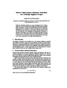
Once the local map is built and aligned with the horizontal plane, we proceed with the last step, that is, the obstacle detection and classification. First of all, → we must approximate the user’s 3D moving vector − v t in order to know the direction where we will look for the obstacles (note that the last pose provides the orientation of the camera, which differs from the moving direction). We → extract − v t from the trajectory information as follows. Consider the last pose of the camera pt and the previous one pk with the highest value of k which satisfy ||[xt , yt , zt ]−[xk , yk , zk ]|| > Kvm . Then, the vector → between both points provides our moving direction: − v t = [xt , yt , zt ]−[xk , yk , zk ]. Note that Kvm determines the smoothing of the resulting moving direction. In our experiments, we use Kvm = 0.5m in order to avoid the little local movements of the user that differ from the real displacement. → Using − v t , the last pose pt and the magnitude of the last action at (defined as lt = ||[δxt , δyt , δzt ]||), we can predict the 3D point where the camera could be ∗ ∗ → , zt+1 ] = [xt , yt , zt ] + lt − v t. in the next iteration: p∗t+1 = [x∗t+1 , yt+1

Fig. 4. Obstacle detection and classification. Two boxes are projected in the predicted position of the blind. Here, we show three situations: no obstacles have been detected (left), a common obstacle with points in both boxes (center) and a aerial obstacle(right) where the upper box contains much more points than the lower one.

The next position of the camera p∗t+1 is then used to place two boxes But and Blt with the same volume (adapted to the volume of the user’s body) that represent the upper and the lower body of the user respectively (see Fig 4 left). Then, we count the number of points of the local map At contained in each box |But | and |Blt |. The aerial obstacle case is detected when the upper box contains much more points than the lower one, that is (1 + |But |)/(1 + |Blt |) > Kr and when this quantity if greater than a threshold |But | > Knp . In this case, the user is notified by a high frequency sound. In other case, no warning is produced (when the number of points are similar or the number of points in the bottom box is greater, the obstacle could be detected by the walking stick). In Fig. 4 we show some representative situations.

11

3

Experimental Results

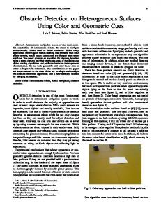
In this section we show the benefits and limitations of our approach through some selected experiments using real data. In order to perform our experiments, we have built a wearable stereo device that consist of a stereo camera (Bumblebee Stereo Vision SystemT M , distributed by Point Grey Research Inc.) and a smallsize laptop (Intel Centrino Core 2 DUO 1.83GHz 2GB RAM) that we carry in a little backpack (Fig. 5). The whole system weighs approximately two kilograms.

Fig. 5. Wearable stereo device used in our experiments that consists of a Bumblebee stereo camera and a small laptop, carried in a little backpack.

Bumblebee is a binocular stereo head with a 12cm baseline which provides 1024 × 768 × 2 color images at 14fps. The camera is pre-calibrated using Tsai’s classic method [13]. The system provides a software library that solves image acquisition, low level preprocesses, stereo correspondence and 3D reconstruction, with sub-pixel accuracy and different 3D filtering criteria. The parameters of the experiments are described as follows: For the sake of efficiency, we use the minimum resolution of the camera (320 × 240). Given our previous experimental evaluations of the stereo head, our maximum range is 12m, being the average error below 0.91m for such distance. Under this resolution, the camera produces clouds of 10, 000 points on average which are typically reduced to 400 points in the feature extraction step, using |W| = 7 × 7 (size of appearance windows). The minimum number of correspondences to ensure the transformation is set to |M|min = 10. Local map building is performed with a maximum distance of Kdmin = 7.0m. In the obstacle detection step, the distance to estimate the moving vector is Kvm = 0.5m, the ratio between the boxes to classify as an aerial obstacle is set to Kr = 3 and the minimum number of points to consider a obstacle is Knp = 3. The experiments are performed in an outdoor unstructured environment composed by grass and trees. The user followed an only trajectory composed by 753 observations, where only 315 were accepted (the ones whose transformation

12

Fig. 6. Outdoor trajectory in an outdoor unstructured environment. The eight points where an aerial obstacle is detected. See the text for more details.

was meaningful enough), taken along 136.15m. In this case, no egomotion failures have been obtained. Then, the re-initialization of the map was not needed. The environment contains a lot of aerial (tree branches) and common obstacles (tree trunks).

Fig. 7. Number of points contained in the upper (top left) and the lower (bottom left) boxes in each iteration, and the ratio between them (top right). Time consumed by the algorithm in each iteration (bottom right). See the text for more details.

In Fig. 6 we show the eight parts of the environment where the algorithm detects an aerial obstacle. Only seven of them are real aerial obstacles. An only false positive is generated, where a trunk of a palm tree is classified as an aerial obstacle (second row, fourth column), while it should been classified as a common obstacle. Note that in some cases, the obstacle is not captured by the last observation (this is one of the reasons that force to use a local map).

13

In Fig. 7 we show some numerical information about the experiments. In the left part of the figure, we show the number of points contained in the upper (top) and lower (bottom) boxes (|But | and |Blt | respectively) in each iteration, as well as the ratio (1 + |But |)/(1 + |Blt |) (top right). As we can see, the eight aerial obstacles cited above are represented by the peaks with |But | > 2 and a ratio greater than 2. In our implementation, we have divided the algorithm into two parallelized proceses: a first one that solves the local map building (image acquisition, stereo computation and egomotion) and a second one that solves the stabilization of the local map, obstacle detection and classification. The parallelization takes advance from the dual-core processor and the nature of the approach (that allows the separation) in order to minimize the time consumed by the algorithm (this parallelization saves arround a 31% of the computation time with respect to a linear one). At the bottom right part of Fig. 7 we show the time consumed by both processes. The red line represents the time consumed by the local map building process (318ms in average) in each iteration. The blue line represents the time consumed by the local map stabilization and the obstacle detection and clasification (306ms in average). The time consumed by the whole algorithm in each iteration is the maximum of both processes, that is, 364ms in average, that allows to perform the aerial obstacle detection at 2.75f ps.

4

Conclusions and Future Work

In this paper, we propose a novel approach for aerial obstacle detection using a stereo vision camera. The algorithm uses a local 3D map of the surroundings of the user in order to detect and classify the obstacles. The local map is approximated by a 6DOF egomotion algorithm and stabilized by an entropy minimization schema which continuously rectifies the global drift integrated with the trajectory. The use of a local map instead of a global one maintain the memory requirements and the processing time approximately constant. Once the map is built and stabilized, a geometric approach to predict the next pose of the user and detect the possible aerial obstacle is used. At the end of the paper we present some selected experiments, performed with a wearable prototype, in order to test our algorithm in a real situation. Our future research includes a miniaturization of the prototype and a comparison with a 3D infrared camera, which combines infrared and vision technologies. IR cameras are usually more compact, faster and precise than stereo vision ones. Another future research consist of testing our prototype with a real blind in a more dynamic environment (for instance urban scenarios), in order to find all of the exceptional situations of the final user.

5

Acknowledgment

This research is partially funded by the projects the projects TIC2002-02792 and DPI2005-01280 of the Spanish Government.

14

References 1. Olson, C., Matthies, L., Schoppers, M., Maimone, M.: Rover navigation using stereo ego-motion. Robotics and Autonomous System (43) (2003) 215–229 2. Se, S., Lowe, D., Little, J.: Mobile robot localization and mapping with uncertainty using scale-invariant visual landmarks. International Journal of Robotics Research 21(8) (2002) 735–758 3. Lowe, D.: Object recognition from local scale-invariant features. In: Proceedings of the International Conference on Computer Vision, Corfu, Greece (September 1999) 4. Ihrke, I.: Digital elevation mapping using stereoscopic vision. PhD thesis, Royal Institute of Technology (2001) 5. Besl, P., McKay, N.: A method for registration of 3D shapes. IEEE Transactions on Pattern Analysis and Machine Intellitence 2(14) (1992) 239–256 6. S´ aez, J., Escolano, F., Pe˜ nalver, A.: First steps towards stereo-based 6DOF SLAM for the visually impaired. In: Proceedings of the IEEE International Conference on Computer Vision and Pattern Recognition, San Diego, USA (June 2005) 7. S´ aez, J., Escolano, F.: 6DOF entropy minimization SLAM. In: Proceedings of IEEE International Conference on Robotics and Automation, Orlando, Florida (May 2006) 8. Se, S., Brady, M.: Stereo vision-based obstacle detection for partially sighted people. In: Proceedings of the Third Asian Conference on Computer Vision, Hong Kong, China (January 1998) 9. Coughlan, J., Shen, H.: Terrain analysis for blind weelchairs users: Computer vision algorithms for finding curbs and other negative obstacles. In: Proceedings of the Conference and Workshop on Assistive Technology for People with Vision and Hearing Impairments, Granada, Spain (August 2007) 10. Komodakis, N., Panagiotakis, C., Tziritas, G.: 3D visual reconstruction of large scale natural sites and their fauna. Signal Processing: Image Communication 20 (2005) 869–890 11. Hero, A., Michel, O.: Asymptotic theory of greedy aproximations to minimal kpoint random graphs. IEEE Transactions on Information Theory 45(6) (1999) 1921–1939 12. Chen, H., Meer, P.: Robust regression with projection based m-estimators. In: Proceedings of the IEEE International Conference on Computer Vision, Nice, France (October 2003) 13. Tsai, R.: A versatile camera calibration technique for high-accuracy 3D machine vision metrology using off-the-shelf tv cameras and lenses. IEEE Journal of Robotics and Automation 3(4) (1987) 323–344