Obstacle Detection Using Adaptive Color Segmentation ... - CiteSeerX

Obstacle Detection Using Adaptive Color Segmentation and Color Stereo Homography Parag H. Batavia and Sanjiv Singh [parag/ssingh]@ri.cmu.edu Carnegie Mellon University Robotics Institute Pittsburgh, PA 15213

Abstract Obstacle detection is a key component of autonomous systems. In particular, when dealing with large robots in unstructured environments, robust obstacle detection is vital. In this paper, we describe an obstacle detection methodology which combines two complimentary methods: adaptive color segmentation, and stereo-based color homography. This algorithm is particularly suited for environments in which the terrain is relatively flat and of roughly the same color. We will show results in applying this method to an autonomous outdoor robot.

1. Introduction This paper describes an obstacle detection algorithm for use in relatively flat areas where there is similarity in color. The method is robust to false positives and negatives through the use of two complimentary methods: color segmentation and color homography. Color segmentation, as the name implies, uses color to classify image areas as “obstacle” or “freespace” The method we use is based on a training algorithm, in which examples of “freespace” are shown to the system, and it learns appropriate representations. Stereo-based homography is often referred to as “poor man’s stereo”. Although computationally cheap, it does not provide depth information, as pure stereo does. Rather, it provides information on whether a particular image feature rises above the ground plane. In applications where a complete depth map is not needed, this can be a computationally cheap alternative. We extend the homography formulation to make use of color information, which improves robustness. This system is used to automatically train the color segmentation system. In the rest of this paper, we describe how both methods are combined to form a robust obstacle detection system, followed by an example of its use on an outdoor mobile robot.

2. Obstacle Detection Obstacle detection is a key component of an autonomous robot, particularly when dealing with large outdoor vehicles. The robot has to have very robust obstacle detection capabilities, since it is a heavy, potentially

dangerous piece of equipment. The size of obstacles can vary, and the detection system has to operate reliably in various lighting conditions, along with light fog and rain, and at night as well. We have examined two methods for detecting obstacles, along with methods for integration of these two methods.

2.1. Color Segmentation The basic idea behind color segmentation for obstacle detection is that pixels in an image are classified as “obstacle” or “freespace” based on color. When operating in domains in which traversable areas are of relatively constant color, such as grass, color segmentation works well. Each pixel in a color image consists of a 3-tuple, representing the amount of energy contained in the red, green, and blue bands. Typically, each component of the tuple is a value between 0 and 255. Therefore, one simplistic method of color segmentation is a rule-based system. In such a system, various rules would be used to classify pixels, such as “if red is between 100 and 175 and green is less than 25 and blue is more than 70, then classify as freespace”. While conceptually simple and extremely fast, such methods are not general. They are specific to lighting conditions, and camera performance, and can easily be fooled by shadows and variations in grass condition. Therefore, we use a general, non-parametric representation similar to that used by Ollis [6] and Ulrich [12], but with extensions for automated training and adaptation. This approach uses a probabilistic formulation to classify pixels, based on a set of training images. These images are not stored as standard (R,G,B) tuples. Rather, they are first converted to a different color space, known as Hue-Saturation-Value, or HSV. This is a cylindrical space, in which the H and S components contain the color information, in the form of a standard color wheel. The Hue is the actual color, or the angle of the point in the cylinder, the Saturation is the “purity” of the color, and is the radial distance of the point. The Value is the intensity, or brightness, and is the height of the point. This space has the advantage that if we ignore the Value

component, we get additional robustness to shadows and illumination changes, along with a reduction in feature dimensionality. Other researchers have addressed the problem of color segmentation. Hyams [3] uses a Spherical Coordinate Transform, which is a color space previously used in the medical domain, combined with a nearest-neighbor segmentation scheme to localize daughter vehicles with respect to a mothership. Shiji [9] uses a watershed algorithm along with extensions to avoid over-segmentation. McKenna [5] uses an adaptive mixture model to represent classes, which is a more compact representation than ours, but is computationally more expensive to train. The dichromatic reflection model, originally proposed by Shafer [8], is still used as well, as seen in [4].

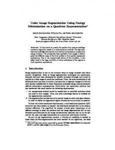
Training Images

Training Histogram

Test Image

Testing Histogram

2.1.1. Training The training set is represented as a two dimensional histogram. The bins in the histogram are addressed based on the H and S values of a color pixel. The contents of the bin denote the number of occurrences of that particular H and S pair in the training set. The color segmentation system has to “learn” what colors constitute traversable areas, such as grass. To train the classifier, we present it with several images of grass taken in various lighting conditions. For each pixel in the training image, the value of the corresponding histogram bin is incremented. Therefore, colors that occur often will have high values in the histogram. After training is done, the histogram is normalized by the total number of samples (i.e., the sum of the bin contents), so that bin contents now represent a probability. The top third of Figure 1 illustrates the training procedure. The top-left image shows a set of training images of grass. The color values contained in these images are added to the histogram, which is shown in the top-right image. The histogram is represented as a color wheel. The area to the right of the center of the wheel, which corresponds to various shades of green, shows activity, which represents the colors in the training set. The training time is linear in the number of image pixels, and in practice is extremely fast. The training can be done in a supervised manner by showing examples of freespace. Alternatively, the training set can be automatically acquired and adapted using homography, a complementary method

2.1.2. Run-Time After training, the system is ready to classify pixels as obstacle or freespace. For each pixel, p, in a test image, we look up the bin value corresponding to the color of p. This provides us with a probabilistic measure, P, of p

Obstacle Image Figure 1: Color Segmentation training and histogram details.

being in the training set. If P is greater than a threshold, then we classify it as freespace. Else, it is an obstacle. I.e, anything which is not freespace is classified as an obstacle. This can lead to false positives, as we will discuss later. The middle third of Figure 1 shows a test image, which contains grass and a bag. The figure on the middle-right shows the color distribution of the test image, again represented as a color wheel. Notice that although a large portion of the test image color distribution overlaps the training set color distribution, there is a significant portion which does not. This portion is due to the presence of the bag. The lower right figure shows an “obstacle image,” in which white indicates obstacle and black indicates freespace. The bag is accurately detected, and there are no false positives.

2.1.3. Performance Color segmentation relies on having a complete training set. As lighting changes, due to time of day or weather conditions, the appearance of grass and obstacle change as well, since the amount of incident sunlight changes. The color of grass is different under a cloud cover than under direct sunlight, and is different in the morning vs. mid-day. This can lead to false positives, if the system is only trained in one lighting condition, and then is used

in another. Since training is so fast, and can be done on the fly, this is not a severe issue. If the environmental lighting changes, we can simply re-train and continue. Similarly, color segmentation can classify flat objects, such as fall leaves, as obstacles, since their color is different from grass. In these cases, it is safe to drive over them. Therefore, there are four possible cases: 1) No obstacle, 2) true obstacle with significant height, 3) true flat obstacle, and 4) false obstacle due to lighting change. In cases 1 and 2, we do not need to modify the training set. In case three, we do not want to modify the training set, but want to recognize that it is safe to proceed. In case 4, we need to augment our training set to handle the new environmental conditions. The next section describes stereo homography, which is a computationally cheap yet powerful method for detecting objects which rise above the ground plane. Homography can provide enough information to disambiguate between cases 2 and 3 or 4.

2.2. Color Homography In conventional stereo, multiple cameras are used to find the range to image features. This range information comes at a steep computational cost. Computing depth using stereo is of the order O(m*n*d), where m is the number of image pixels, n is the size of the correlation window, and d is the number of disparities searched, which is related to the range of depths which can be found. Another way to find obstacles is to use homography, which is linear in the number of image pixels. This is because homography does not compute range. Rather, it provides just enough information to determine whether a particular image feature is on the ground or above it. The basic idea behind homography is this: If we know the extrinsic and intrinsic parameters of both cameras, and assume that all image features lie on the ground plane, we can solve the inverse perspective problem. I.e., any given image point in the [left/right] camera can now be back-projected into world coordinates. These world coordinates can then be forward-projected into the opposite camera. Using the left camera as an example, we can warp the left camera image to the right camera, and then compare the warped image against what the right camera actually sees. If all the image features actually do lie on the ground plane, then the warped image will match the actual right camera image. However, if certain image features lie above the ground plane, then our warped image will be incorrect in those areas, and this discrepancy can be detected.

Figure 2: Homography calibration images.

Previous work, as described in the next section, has made use of grey scale intensity images. Often, objects of different colors have the same intensity as the ground plane. In these cases, detecting ground plane violations through image subtraction fails. To avoid this, we use hue images, which capture the color properties of the background and potential obstacles.

2.2.1. Image Warping We do a perspective warping of the left image to the right image, based on a 3x3 homography matrix. The equation to do the warping is:

x' = Hx

(1)

Where x’ is the (u,v,1) homogenous coordinate of the left image, x, and H is the homography matrix. H is determined through a calibration procedure, described fully in [11], in which an image pair is taken, and a small set (usually four) of corresponding features in the left and right image are manually selected. These features must lie on the ground plane. A sample pair of calibration images is shown in Figure 2. Typical features to mark would be the corners of the white calibration markings. Four corresponding features provides enough constraints to solve for the 8 free parameters in H (the 3,3 element of H is always 1). However, in practice, this yields a sub-optimal solution. Therefore, a levenbergmarquardt non-linear optimization step is applied to find the optimal value for H. Once calibration is accomplished and H is found, obstacles can be detected. Figure 3 shows an example of homography being used for obstacle detection. The top-left and top-right images are the left and right camera input images, respectively. The bottom-left image is the left image, warped as it would be seen from the right camera, given the assumption that all features lie on the ground. Note that there is a triangular black area in the warped image, on the right side. This is due to a lack of information, since the left camera field of view does not extend as far right as the right camera field of view. The bottom-right image is a thresholded

2.3. Integration Given two working, complimentary, obstacle detection methods, integration is an issue. Both methods have different strengths and weaknesses, and it is important to integrate them in such a way that the strengths of each are used to offset the respective weaknesses. For instance, color segmentation, although able to detect small obstacles and changes in color, is not sensitive to obstacle geometry, such as height. Homography is only able to find obstacles that are over a certain height. Both methods produce a list of candidate obstacles and centroid locations. It would be possible to just combine them in an ‘OR’ fashion. Alternatively, they could be ‘AND’ed, so that both methods would have to detect a particular obstacle. Figure 3: Homography example. The top images are input images. The bottom left image is a warped image. The bottom right image is the obstacle image.

difference image between the right camera image and the warped image. The two white areas in the difference image correspond to the portions of the obstacle which did not match the prediction, since it lies above the ground plane. Previous work includes work by Storjohann [10], for indoor applications of homography and inverse perspective mapping. Batavia [1] has used a monocular version of homography, utilizing a single camera and known ego-motion, rather than two cameras, for highway obstacle detection. Santos-Victor [7] also used a monocular approach, but with a formulation that did not require knowledge of ego-motion. However, this approach requires the computation of normal-flow vectors. Bertozzi [2] used a stereo approach for detecting highway obstacles, with an on-line calibration-tuning ability.

2.2.2. Performance This method is robust to the types of false positives which confound color segmentation. The sensitivity to true obstacles is determined by the image resolution, calibration accuracy, and field of view. This can be improved by increasing the image resolution and/or narrowing the field of view. In general, the same issues which affect stereo accuracy have an impact on homography accuracy. Another issue is sensitivity to pitch variations. This variation can come from platform vibration, or it can come from a change in the terrain slope, which breaks the ground plane assumption. Large deviations in pitch from the calibrated conditions can lead to false positives, as the image warping process is dependant on a pre-determined pose.

We use homography to act as a ‘false positive’ filter for color segmentation. When color segmentation detects an obstacle, homography is used to decide whether the obstacle is rising above the ground or not. If it is, then the object is classified as an obstacle. If it is not, then a decision has to be made whether to adaptively re-train the color segmentation system (in the case of global lighting change) or whether to simply ignore the object, assuming it is a temporary obstacle (such as a leaf). This decision is made based on the size of the obstacle. If it is extremely large, subtending most of the image, then it is likely that there is no object at all, and it is a global lighting change, and we re-train. Using homography as a filter allows us to adaptively re-train on the fly, without operator intervention.

3. Experimental Results We have tested the fully integrated obstacle detection system offline, on image sequences, and online, using a mobile robot. We have also done extended duration testing using only color segmentation. The platform we use for online testing is described in the next section

3.1. Platform Description The platform used for these experiments is a riding lawnmower and is pictured in Figure 4. The front bumper contains two CCD cameras and a SICK laser scanner. Currently, an integrated PC, mounted in the rear, is used to communicate with the sensors and control the vehicle. The steering and throttle are hydraulically controlled, and are both actuated. A serial protocol is used to set steering and throttle positions. The planner and trajectory generation module takes pose information as input, and generates trajectory commands as output, and

False Obstacle Difference Image Histogram 3000

Figure 4: Riding lawnmower with cameras and laser range finder.

passes them to the command and safety arbiter, which executes commands, based on input from the obstacle detection subsystem. A dead-reckoning system is used for navigation, which integrates odometry information from two wheelmounted encoders, along with heading information from a fiber optic rate gyro. Dead-reckoning will accumulate error over time. Over large distances, some form of globally-referenced localization will be required to bound the dead-reckoning error.

3.2. Results The first test involves offline processing of two image sequences. The first sequence contains one true obstacle -- a small red fire extinguisher, and is the same sequence of Figure 3. The second sequence contains a false positive -- a large area of discolored grass and sand. Figure 5 shows results from the two sequences. The top two images are the left and right camera images of the sand sequence. The middle left image is the color segmentation output on the left input image. The middle right image is a histogram of the homography difference image. Recall, the difference image is an absolute difference between the hue of the actual right input and the hue of the warped image. The bin centers are difference values, and the counts indicate the number of pixels in the difference image which fell into the corresponding bin. Peaks at high difference values indicate the presence of an obstacle. The middle right figure shows only a peak at very low difference values, indicating that homography does not detect an obstacle. Therefore, the output of the color segmentation is actually a false positive. In contrast, the bottom two figures show an input image from the fire extinguisher sequence, and the corresponding difference histogram. Note the peak at higher difference values. This indicates the presence of an obstacle. The output of the color segmentation is true in this case.

0 0

Difference Value

90

True Obstacle Difference Image Histogram 3000

0

0

Difference Value

90

Figure 5: Offline homography results on true obstacle vs. false positive.

Our online testing made use of the lawnmower platform. The robot navigated autonomously through an oval pattern, travelling a total of 200m over 7 minutes. The color segmentation system starts with an initial training set of one image of grass. During this period, a “false obstacle,” in the form of a green sheet, was set in front of the path. Figure 6 shows this. This sheet is meant to represent an area of grass which is of different color than the grass initially used for training. If operating alone, a human operator would have to decide whether or not to augment the training set with the new grass, since it appears as an obstacle. Instead, color homography is used to validate the color segmentation output. The sheet is flat on the ground, so the homography prediction matches what is actually observed. Therefore, the object is declared a false positive. The decision to add this image to the color segmentation training set is made because the object is larger than a thresholded size. If the object had been smaller, it would have been ignored, and the mower would have continued.

3.3. Extended Duration Results We conducted another test during a recent demonstration of the color segmentation system. In this test, only color segmentation was used. The mower runs in straight swaths of about 10 meters, then turns 180

along with accurate localization, the inverse perspective equations are solvable for arbitrary terrain. Also, the color segmentation can be improved through additional color-constancy work. In particular, accounting for the spectral contribution of varying sunlight should greatly reduce the number of false positives.

References

Figure 6: A green sheet simulating an area of new grass. The lower left image is a depiction of the training set before the new grass was added. The lower right is the training set after it was added.

degrees and repeats the pattern. The total distance travelled in this case is about 60 meters, and the total area mowed is about 80 square meters. Over a recent four day period, we repeated this pattern approximately 50 times, resulting in a total distanced travelled of about 3 km., and a total area covered of about 4 square km. Over these 50 trials, false positives were encountered on average of once every 250m of travel. True obstacles were also placed in its path, with 100% detection.

4. Conclusion and Future Work We have demonstrated a novel integration of two visionbased obstacle detection methodologies: color segmentation, and color homography. Each method has strengths which compensate for the other’s weaknesses, resulting in a robust method for obstacle detection. Furthermore, the homography is used to autonomously train the color segmentation system, allowing unsupervised training. Future work includes further improving the robustness of the obstacle detection system and navigation system to allow for unattended operation over larger areas, on the order of 10 to 20 square kilometers. In particular, the homography approach is not limited to flat ground. Given terrain information, in the form of a digital map,

[1] P. Batavia and D. Pomerleau and C. Thorpe, “Overtaking Vehicle Detection Using Implicit Optical Flow,” Proceedings of the IEEE Intelligent Transportation Systems Conference, Boston, MA, 1997. [2] M. Bertozzi and A. Broggi and A. Fascioli, “Stereo Inverse Perspective Mapping: Theory and Applications,” Image and Vision Computing, Vol 16, pp. 585-590, 1998. [3] J. Hyams and M. Powell and R. Murphy, “Cooperative Navigation of Micro-rovers using Color Segmentation,’ Journal of Autonomous Robots, Vol. 9, Num. 1, pp 7-16, August, 2000. [4] V. Kravtchenko and J. Little, “Efficient Color Object Segmentation Using the Dichromatic Reflection Model,” Proceedings of the IEEE Pacific Rim Conference on Communications, Computers, and Signal Processing, 1999. [5] S. McKenna and Y. Raja and S. Gong, “Tracking Color Objects Using Adaptive Mixture Models,” Image and Vision Computing 17, pp. 225-231, 1999. [6] M. Ollis, “Perception Algorithms for a Harvesting Robot,” Carnegie Mellon University Doctoral Dissertation, CMURI-TR-97-43, August, 1997. [7] J. Santos-Victor and G. Sandini, “Uncalibrated Obstacle Detection Using Normal Flow,” Machine Vision and Applications, Vol 9, pp 130-137, 1996. [8] S. Shafer, “Using Color to Separate Reflection Components, “Color Research, Vol. 10, Num. 4, pp 210-128, 1985. [9] A. Shiji and N. Hamada, “Color Image Segmentation Method Using Watershed Algorithm and Contour Information,” Proceedings of the International Conference on Image Processing, Kobe, Japan, October, 1999. [10] K. Storjohann and T. Zielke and H.A. Mallot and W. von Seelen, “Visual Obstacle Detection for Automatically Guided Vehicles,” Proceedings of the International Conference on Robotics and Automation, pp 761-766, 1990. [11] T. Williamson, “A High-Performance Stereo System for Obstacle Detection,” Carnegie Mellon University Doctoral Dissertation, CMU-RI-TR-98-24, September, 1998. [12] I. Ulrich and I. Nourbakhsh, “Appearance-Based Obstacle Detection,” AAAI National Conference on Artificial Intelligence, Austin, TX, August 2000.

Acknowledgements The authors would like to acknowledge the support of Iwan Ulrich, whose work provided the foundation for the color segmentation-based obstacle detection system described here, along with lower level camera driver support.