labels, the probability of a random walker starting from an unlabeled node u and .... where we take θ1 = 0.03,θ2 = max{0.1Yavg â. 0.04, 10â4}, Î = 150. C(pi, d) ...
Stereo Matching Using Random Walks Rui Shen, Irene Cheng, Xiaobo Li and Anup Basu Department of Computing Science, University of Alberta, Canada {rshen,lin,li,anup}@cs.ualberta.ca
Abstract This paper presents a novel two-phase stereo matching algorithm using the random walks framework. At first, a set of reliable matching pixels is extracted with prior matrices defined on the penalties of different disparity configurations and Laplacian matrices defined on the neighbourhood information of pixels. Following this, using the reliable set as seeds, the disparities of unreliable regions are determined by solving a Dirichlet problem. The variance of illumination across different images is taken into account when building the prior matrices and the Laplacian matrices, which improves the accuracy of the resulting disparity maps. Even though random walks have been used in other applications, our work is the first application of random walks in stereo matching. The proposed algorithm demonstrates good performance using the Middlebury stereo datasets.
1. Introduction Stereo vision is a very active research area in computer vision. One crucial and traditional task in stereo vision is stereo matching, the goal of which is to determine the disparities of corresponding pixels in a pair of stereo images. Many algorithms have been proposed to solve this problem. According to the comprehensive survey by Scharstein and Szeliski [8], the existing algorithms can be roughly classified into two categories: local (window-based) algorithms [1] that compute disparities within a finite window, and global algorithms [1] that find the best disparity configuration by minimizing a global energy function. Compared with local methods, global methods produce more accurate results using optimization frameworks, such as graph cuts (GC) [1], belief propagation (BP) [6] and dynamic programming (DP) [7]. A recent application of random walks (RW) in multilabel image segmentation [2][4] shows great potential
978-1-4244-2175-6/08/$25.00 ©2008 IEEE
for its application in stereo matching. As shown in [3], RW demonstrates superior performance over GC in segmentation. The segmentation is achieved by minimizing the Dirichlet integral, which is actually a kind of energy function that can be defined in the form of the typical energy function used by global stereo algorithms: E( f ) = Edata ( f ) + λEsmooth ( f ).
(1)
The major advantage of random walks is that an exact and unique minimum solution of an energy function of the above form can be produced, while other approaches like GC can only produce an approximation. Therefore, it is very likely that RW can achieve better performance than GC and other optimization frameworks in stereo matching. Hence, we develop a new stereo matching algorithm using random walks. Our contribution lies in that our work is the first application of random walks in the area of stereo matching. Two major phases are considered: first, a set of reliable matching pixels is computed using RW with prior models [2] (Section 4); second, with the reliable set serving as seeds, the disparities of unreliable pixels are determined using the original RW [4] (Section 5). As demonstrated in Section 6, our algorithm produces more accurate disparity maps than many of GC-based and DPbased methods, and some of BP-based methods.
2. Random walks Random walks works on a graph representation G = (V , E) of an image, where V is the set of all the pixels and E is the set of weighted edges. Given a set S of k labels, the probability of a random walker starting from an unlabeled node u and reaching a seed (labeled node) is calculated. u is assigned a label s, if it has the highest probability of reaching a seed with label s. The calculation of the probabilities is equivalent to the Dirichlet problem, and the solution can be found by solving the equation: (2) LU x s = − B T f s ,
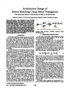
Figure 1. Processing procedure of the proposed algorithm. where xs is the vector to be calculated that represents the probability of each unlabeled node being assigned label s. LU is a submatrix of the Laplacian matrix L, containing weights of the edges connecting unlabeled nodes. B T is another submatrix of L, containing weights of the edges connecting a seed and an unlabeled node. f s is a binary function defined on V and S. Prior terms can also be incorporated using the improved RW algorithm [2]. In addition to L, a set of priors {λis } is added to represent the probability that a node vi belongs to label s. Then, the segmentation (labeling) problem can be formulated as minimizing an energy function of the form: Estotal = Esspatial + γEsaspatial .
(3)
Note the resemblance of Equation 3 to Equation 1. The solution is obtained by solving the equation: k
(L + γ
∑ Λ r ) xs = λ s ,
(4)
r=1
where Λ = diag(λ s ). We term the matrix containing all the priors as the prior matrix P = [λis ].
the YCb Cr space, and the parameters are adjusted automatically according to the illumination condition of the input image pair.
4. Reliable matching pixel computation In order to formulate the stereo matching problem in the RW framework, the Laplacian matrix L and the prior matrix P need to be built first. The weight of an edge connecting pixel pi and pixel p j is defined as: wi j = e−βk pi − p j k + �,
(5)
where k pi − p j k is the Euclidean distance between pi and p j in the YCb Cr space, and � (we set � = 10−5 ) is a small positive constant. In practice, k pi − p j k is normalized between [0, 1]. β is a weighting factor to reduce the effect of variance of illumination across different images. Intuitively, the lower the brightness of an image, the smaller the difference between similar pixels in the YCb Cr space; thus, a larger β is needed to emphasize the difference. We use the average luminance value Yavg as the measurement of the brightness of an image. Hence, β is adjusted according to the equation:
3. Algorithm overview β = max(βini − δβ Yavg , θβ ), Like graph cuts [1], we define the set of labels as the set of all possible disparities between [0, dmax ]. Thus, the stereo matching problem is formulated in the RW framework as finding the minimum of Equation 3. The whole procedure is illustrated in Figure 1. An initial disparity estimation for both images (Il and Ir ) is obtained by solving Equation 4. Left-right checking (Section 4.1) is applied to determine a set of reliable matching pixels. Unreliable pixels are marked in black in Figure 1(c)(d). Special consideration is given to textureless regions (marked in white in Figure 1(c)). Using the intermediate result, an optimal disparity map is computed by solving Equation 2. Between each step, the intermediate disparity maps are smoothed (e.g., using a median filter) to reduce noise. Our algorithm works in
(6)
where we set βini = 295, δβ = 380, θβ = 0.1δβ . After calculating all the edge weights, the Laplacian matrix L is built using the equation from [4]: ∑k wik , i = j; − wi j , pi and p j are adjacent; (7) Li j = 0, otherwise. To build the prior matrix P, a prior λid is defined as: Θ, λid = e−σ (0.1θ2 ) , −σC( p ,d) i , e
mind∈[0,dmax ] {C ( pi , d)} ≥ θ1 ; C ( pi , d ) ≤ θ 2 ; otherwise. (8)
where we take θ1 = 0.03, θ2 = max{0.1Yavg − 0.04, 10−4 }, Θ = 150. C ( pi , d) is defined in a similar way as in [1] using the pixel dissimilarity measure: C ( pi , d) = min{C f wd ( pi , d), Crev ( pi , d)}.
(9)
In practice, C ( pi , d) is normalized between [0, 1]. We found that Crev ( pi , d) only calculated for the reference image is sufficient for a final disparity map with comparable quality. Like β, σ is determined by: σ = max(σini − δσ Yavg , θσ ),
If pm is found, db = dm ; otherwise, db is unchanged. The remaining pixels of R are categorized into U.
5. Unreliable pixel labeling The disparity assignment of unreliable pixels U based on the disparities of reliable pixels M is exactly the same as the Dirichlet problem defined in the original RW framework [4]. f id is defined as:
(10)
where we set σini = 499, δσ = 720, θσ = 0.1δσ . Given L and P, the probability xid of a pixel being assigned a disparity d ∈ [0, dmax ] can be calculated by solving Equation 4, where we set γ = 10−5 . Pixel pi is assigned the disparity d with the highest probability, i.e., D ( pi ) = arg maxd ( xid ), ∀d.
4.1. Left-right checking A left-right checking technique similar to the one used in [7] is applied to extract a set M of reliable matching pixels. The remaining pixels are categorized into the unreliable set U. Since the left image Il is used as the reference image, this reliable set is only determined on Il . For two matching pixels ( pl , dl ) ∈ Il and ( pr , dr ) ∈ Ir in the two images (i.e., pr .x = pl .x + dl and pr .y = pl .y), the reliability of ( pl , dl ) is determined by: � M, dl ∈ [−dr − θ3 , −dr ]; (11) ( pl , dl ) ∈ U, otherwise. d0
0 where we take θ3 = d max 7 e with dmax as the maximum disparity in the initial disparity maps. Pixels with d0 pl .x ≤ b max 2 c are directly labeled as unreliable without left-right checking, because they are occluded in Ir .
4.2. Textureless region handling Textureless regions tend to cause wrong disparity estimation. Due to the high similarity of a pixel to its neighbouring pixels, a small disparity is very likely to be assigned while the true disparity may be much larger. Therefore, after left-right checking, every pixel ( pb , db ) on the left boundary of a region R ⊂ M with disparity d ≤ θ3 , ∀( p, d) ∈ R is selected to go through a disparity validation test. The validation procedure is d0 simply a linear search from max{ pb .x − 1, d max 2 e} to d0
max{ pb .x − d0max , d max 2 e} to find the matching pixel pm in Ir with the largest disparity dm that satisfies:
k pb − p j k ≤ θ2 , ∀ p j ( p j .x ∈ [ pb .x − dm , pb .x − 1]). (12)
f id
�
=
1, 0,
(( pi , di ) ∈ V ) (di = d); otherwise. V
(13)
Matrices LU and B T are obtained by reformatting L as: � � LM B . (14) L= B T LU After this step, the disparities of unreliable pixels are computed by solving Equation 2.
6. Experimental results & discussion Our algorithm was evaluated using the Middlebury test bed (http://vision.middlebury.edu/stereo/) designed by the authors of [8]. A set of constant parameters is used for all images. The current ranking of our algorithm is 17th among 41, and it is compared with top three algorithms in Table 1. Each decimal entry from the third column to the last column represents the percentage of bad pixels for different regions with absolute disparity error larger than one pixel. The disparity maps (top row) are shown against the ground truths (bottom row) in Figure 2. The computational complexity of RW is O(n) as given in [2]. As our algorithm mainly works by solving two consecutive Dirichlet problems using the RW framework, its computational complexity is also O(n). Our algorithm is currently implemented in Matlab. The computational time ranges from 17 (Tsukuba) to 41 seconds (Teddy) on a 2.41GHz Athlon 64 dual-core computer with 2GB memory. The most time-consuming part is building P, which takes between 4 (Tsukuba) and 21 seconds (Teddy). A C++ or GPU (graphics processing unit) implementation would be much faster. Besides this, solving the Dirichlet problems takes between 11 (Tsukuba) and 17 seconds (Teddy). A GPU implementation of random walks was proposed in [5], which demonstrated an approximately 10-fold speedup. Therefore, we expect at least a 10-time speedup once our algorithm is implemented in GPU, which will be significantly faster than many other global methods using a different optimization framework (e.g., [1][6][7]).
Table 1. The Middlebury stereo evaluation results of the proposed algorithm. Algorithm
nonocc
all
disc
nonocc
all
disc
nonocc
all
disc
nonocc
all
disc
DoubleBP2
Avg. Rank 2.8
0.88?
1.29
4.76
0.13
0.45
1.87
3.53
8.30
9.63
2.90
8.78
7.79
1∗
1
1
3
5
5
2
3
1
3
7
2
AdaptingBP [6]
3.0
1.11
1.37
5.79
0.10
0.21
1.44
4.22
7.06
11.8
2.48
7.92
7.32
7
3
8
1
2
1
4
2
4
1
2
1
DoubleBP
4.8
0.88
1.29
4.76
0.14
0.60
2.00
3.55
8.71
9.70
2.90
9.24
7.80
2
2
2
5
12
7
3
5
2
4
10
3
... 0.96
... 1.47
... 4.91
... 1.41
... 1.71
... 3.46
... 7.83
... 13.2
... 17.8
... 5.76
... 11.6
... 11.8
4
5
3
27
23
16
19
17
18
28
25
22
... Proposed Algorithm
... 17.2
Tsukuba
Venus
Teddy
Cones
∗: The subscripted integers are the ranks of each algorithm in each column; ?: percentage (%) of bad pixels.
Figure 2. Dense disparity maps for the Middlebury stereo datasets. Our results are in the top row and the ground truths are in the bottom row.
7. Conclusion In this paper, we not only proposed a new algorithm for stereo matching, but also demonstrated the feasibility of a new framework, random walks, for solving the stereo matching problem. The major parameters (β and σ) used in our algorithm are adapted automatically according to the illumination condition of the input image pair. The evaluation results of our algorithm using the Middlebury datasets demonstrated promising performance. One limitation of our algorithm is that it works in the YCb Cr space, which limits it to color images. In the future, we plan to incorporate segmentbased methods (e.g., [6]) to label a more reliable set of initial matching pixels, which will be used to initialize the random walks optimization procedure. This combination, together with GPU implementation, will achieve a much more accurate and faster disparity estimation.
References [1] Y. Boykov, O. Veksler, and R. Zabih. Fast approximate energy minimization via graph cuts. IEEE PAMI,
23(11):1222–1239, 2001. [2] L. Grady. Multilabel random walker image segmentation using prior models. In Proceedings of CVPR’05, pages 763–770, 2005. [3] L. Grady. Random walks for image segmentation. IEEE PAMI, 28(11):1768–1783, 2006. [4] L. Grady and G. Funka-Lea. Multi-label image segmentation for medical applications based on graph-theoretic electrical potentials. In Proceedings of ECCV’04 Workshops on CVAMIA and MMBIA, pages 230–245, 2004. [5] L. Grady, T. Schiwietz, S. Aharon, and R. Westermann. Random walks for interactive organ segmentation in two and three dimensions: implementation and validation. In Proceedings of MICCAI’05, pages 773–780, 2005. [6] A. Klaus, M. Sormann, and K. Karner. Segmentbased stereo matching using belief propagation and a self-adapting dissimilarity measure. In Proceedings of ICPR’06, pages 15–18, 2006. [7] C. Lei, J. Selzer, and Y.-H. Yang. Region-tree based stereo using dynamic programming optimization. In Proceedings of CVPR’06, pages 2378–238, 2006. [8] D. Scharstein and R. Szeliski. A taxonomy and evaluation of dense two-frame stereo correspondence algorithms. IJCV, 47(1-3):7–42, 2002.