OR static response, the condition number of the stiffness. F matrix is an upper bound to the amplification of errors in structural properties and loads. However ...
1322
AIAA JOURNAL
4Bahar, L. Y., and Hetnarski, R. B., “Coupled Thermoelasticity of a Layered Medium,” Journal of Thermal Stresses, Vol. 3, April 1980, pp. 141-152. 5Takeuti, Y. and Tsuji, M., “Thermal Stress Problems in Industry, Part 6: Transient Thermal Stresses in a Plate due to Rolling with Considerations of Coupling Effect,” Journal of Thermal Stresses, Vol. 5 , Jan. 1982, pp. 53-65. 6Takeuti, Y., and Furkawa, T., “Some Considerations on Thermal Shock Problems in a Plate,” Journal of Applied Mechanics, Vol. 48, March 1981, pp. 113-118. ’Takeuti, Y., and Furkawa, T., “Some Considerations on Thermal Shock Problems in a Plate,” Journal of Thermal Stresses, Vol. 4, 1981, pp. 461-478. sChen, Y., Ghoneim, H., and Chen, Yu, “A Finite Element Solution of the Coupled Thermoelasticity Equations in A Slab,” Advances in Computer Technology, A S M E , Vol. 2, 1980, pp. 199-218. 9Li, Y. Y., Ghoneim, H., and Chen, Y., “A Numerical Method in Solving a Coupled Thermoelasticity Equation and Some Results,” Journal of Thermal Stresses, Vol. 6, April 1983, pp. 253-280.
Stiffness-Matrix Condition Number and Shape Sensitivity Errors
Raphael T . Haftka* Virginia Polytechnic Institute and State University Blacksburg, Virginia 24061
Introduction
F
OR static response, the condition number of the stiffness matrix is an upper bound to the amplification of errors in structural properties and loads. However, even though typical stiffness matrices have condition numbers larger than one million, we do not expect that errors or variations in the structure or loads would be amplified so much. The present Note seeks to explain why in most cases our expectation is fulfilled. It also presents an example of a case associated with shape sensitivity analysis where the worst-case scenario predicted by the condition number is much closer to the actual error amplification. A criterion is proposed that is closer to the actual error magnification than the condition number. Consider the discretized equations of equilibrium of static response such as those generated by a finite-element model
Ku=f
(1)
VOL. 28, NO. 7
where hi denotes the ith eigenvalue of K . It is well known (e.g., see Ref. 1) that c ( K ) is an upper bound on the sensitivity of u to perturbations in K and f . That is, if we perturb f by Af then
(4)
and if we perturb K by AK then
The condition number for most stiffness matrices generated by finite-element models runs into the millions. This would appear to indicate that the computed displacement field can be extremely sensitive to small errors in the stiffness matrix and force vectors. In spite of this theoretical sensitivity, we continue to approximate the stiffness matrix (e.g., by reduced integration) and the force vector (e.g., lumping loads) without fear of the huge amplification of errors predicted by the condition number. It is known, in fact, that the condition number may be an overly conservative estimate of error sensitivity.2 The condition number is particularly overconservative for predicting sensitivity to changes in the load vector. For a given K and f , it is always possible to find a AK to make Eq. ( 5 ) an equality. Also, c ( K )can be a good predictor of roundoff error amplification so that if the condition number is lo7 and we work with 7-digit numbers, the errors in u can be very large. In the following it is assumed that the number of digits available for computation is much larger than the condition number (a typical case in finite-element computation is c ( K ) = lo7 with 15-digit computations). However, it is not usually possible to find a Af to make Eq. (4) an equality.2 The present Note derives a sharper estimate for sensitivity to load errors. It also presents a case where the extreme sensitivity predicted by the condition number is more closely realized.
Error Analysis Let the eigenvectors of K be denoted as ui, i = 1,...,n normalized to 11 ui II= 1 with X i being the corresponding eigenvalues. We expand the load vector in terms of the eigenvectors as n
f = &Y;uj i= 1
and similarly the perturbation or error in the load as n
(2)
Aaju;
Af = i= I
(7)
It is then easy to check that u can be obtained as n
where K is the n x n symmetric, positive, definite, stiffness matrix, u the displacement vector, and f the load vector. The condition number of K , c ( K ) is defined as
=llKll IIK-lII
(6)
u
(ai/h;)ui
=
i= 1
with a similar expansion for Au . The error amplification factor e is defined as
when the 2-norm is used
(9) Using the orthonormality of the eigenvectors we get e2 =
Received May 1989; revision received Aug. 1989. Copyright 0 1989 by R. T. Haftka. Published by the American Institute of Aeronautics and Astronautics, Inc., with permission. *Christopher Kraft Professor of Aerospace Engineering and Ocean Engineering, Member AIAA.
(Cy= lAa:/X:)(Cy= la:) (Cy= laf//xf)(Ey=,Acuf)
(10)
It is easy to check that the worst case is when the perturbation is in the shape of the first eigenvector, Af = Aalul so that an upper bound on e , called here the error magnification index
JULY 1990
TECHNIC‘AL NOTES
and denoted e,, is given as
1323
Table 1 Dependence of condition number, error magnification index, and actual errors in semianalytical, tip-rotation derivatives on the number of elements
Equation (11) predicts that the error amplification is large when I(f (1 is large and I(u 11 is small. This will happen when f is in the shape of a combination of higher eigenvectors [see Eqs. (6) and (S)]. For example f can be highly oscillatory in its spatial distribution or in a high, aspect-ratio, beam-type structure, f could correspond to shear loading. For f = a,u, and Af = Aaiul, we get e = e, = h,/h, = c ( K ) (12)
so that when the load is in the shape of the last eigenvector, and the load error is in the shape of the first eigenvector, the error amplification is indeed equal to the condition number. The error magnification index e,,, given by Eq. (1 1) is a much sharper estimate of error amplification than the condition number c ( K ) . In fact, for a force in the shape of the first eigenvector, f = a i u l , Eq. (1 1) gives e, = 1, so that there is no error amplification no matter how high the condition number. Because in most practical situations, f is a linear combination of the first few eigenvectors, e, is much smaller than c ( K ) ,and we do not get large force-error magnification even when the condition number is high.
Application to Shape Sensitivity We can obtain the sensitivity derivative u’ of the displacement with respect to a structural parameter v by differentiating Eq. (1) as Ku’ = - K ’ u ZE f p (13) where a prime denotes a derivative, and it is assumed that f does not depend on structural parameter. The right side of Eq. (13) f p is called the pseudoload, and it is often approximated as K ( v + Av) -K ( v ) f p -K’u U (14)
Derivative w.r.t.L Number of elements
Condition number
1 2 3 4 5 6 7 8 9 10
19.3 420 2200 6900 16,660 34,000 62,400 105,000 167,000 253,000
eda
5.67 49.1 135 273 472 737 1076 1500 2000 2590
Percent error in tip rotation 4 16 35 62 97 140 190 249 314 388
Derivative w.r.t.h eda
Percent error in tip rotation
1.1 1.3 1.5 1.7 1.9 2.0 2.2 2.3 2.4 2.5
1.o 1.0 1.o 1.o 1.o 1.o 1.o 1.o 1.o 1.o
In fact, as m goes to infinity, we get from Eq. (16) that
That is, the derivatives of the displacements and rotations are mismatched in that the derivative of the slope is only one half of the slope of the derivative. This mismatch between w ’ and 8‘ results in a u’ representing a displacement shape where each element is being bent into an s-shape, no matter how many elements we have. When m is large, this is a short-wave displacement shape that would be represented by the last few eigenvectors of K . The error analysis of the previous section would then predict the potential for large error magnification-especially for long-wave errors. The error magnification index for the derivative ed is defined based on Eqs. (11) and (13) as
Av
that is by a forward finite-difference approximation. This approach to calculating u ‘ is called the semianalytic method and is implemented in NASTRAN and other finite-element programs. For beam and platelike structures a semianalytical method can result in large errors due to the approximation of Eq. (14) when u is a shape ~ a r a m e t e r . This ~ . ~ behavior is now analyzed with the aid of the error magnification factor index of Eq. (11). Consider the cantilever beam shown in Fig. 1 . The beam is divided into m finite elements (which yield the exact solution for any m ) . The components of u are the normal displacement w;and slope 81 at the nodes given by
Mi2L2 w. - Mx? -=-
8 . -Mx. 2 = - MiL
2EI 2EIm2’ ‘ - EI mEI’ i = O,l, ...,m (15) The derivatives of wi and Bi with respect to L are , Mi2L - Mx,? , Mi w . =--8. =-=% (16) I EIm2 EIL’ I mEI EIL I -
As was noted in Ref. 4,w’ and 8’ are not matched in the sense that 8‘ is not the slope of w’.
w
I =
(1)
--
-
(2)
t o il
- 1 ) (m) Fig. 1 Geometry, loading, and discretization for cantilever beam. I
(m
The large errors associated with the semianalytical method for shape derivatives are in contrast to the small errors for size or stiffness derivatives. To show that the error magnification index discriminates between the two, we compare the derivative with respect to the length of the beam with the derivative with respect to the height h of the cross section of the beam (assumed to have a rectangular cross section). The pseudoload f p is calculated from Eq. (14) for a change in length or height corresponding to 1% of the nominal value. The error in fp is then of the order of 1%. The effect of number of elements on the error magnification index and the actual error is shown in Table 1 . For derivatives with respect to length, ed increases rapidly with the number of elements lagging behind the condition number by about one to two orders of magnitude. The actual error also increases fast though not as fast as e d . The potential error magnification of ed is not realized because the error in fp due to the finite-difference approximation of Eq. (14) is not in the shape of the lowest eigenvector [which is the worst-case scenario assumed in Eq. (1111. The error magnification index for the height derivative increases very slowly with the number of elements and predicts well the sensitivity of that derivative to errors in the pseudoload. A 1 Yo perturbation in a design variable for the purpose of derivative calculation is too large for most practical examples. However, for this example, the errors in the semianalytical method are almost exactly proportional to the perturbation so that the errors in Table 1 (columns 4 and 6) simply scale as the perturbation size is scaled.
Concluding Remarks An error magnification index was proposed for assessing the sensitivity of the displacement field to errors in the load vector.
1324
AIAA JOURNAL
The index is less conservative than the condition number of the stiffness matrix and reflects the fact that for some cases, no error magnification occurs even when the condition number is very high. The proposed index was applied to calculation of derivatives of beam response to changes in the beam structural parameters by the semianalytical method. The calculation of derivative with respect to length is very sensitive to errors; whereas the calculation of derivative with respect to cross-sectional height is not. The proposed index indiscriminated well between these two cases.
VOL. 28, NO. 7
Condensation of Stiffness and Mass Matrices Free vibration analysis of structures results in a matrix equation of the form
where [ K ]and [MI are the stiffness and mass matrices, respectively, [ U ] is the modal vector, and X is the square of the natural frequency. If this system of equations is partitioned, separating the boundary and internal degrees of freedom, the following equation system is obtained:
Acknowledgments This research was supported by NASA Grant NAG-1-224. Helpful comments from Layne T. Watson and William Greene are greatly appreciated.
From the second row of these matrix equations,
References ‘Golub, G. H., and Van Loan, C. F., Matrix Computations, The Johns Hopkins University Press, Baltimore, 1983. 2Chan, T. F., and Foulser, D. E., “Effectively Well-conditioned Linear Systems,” SIAM Journal of ScientSficand Statistical Computing., Vol. 9, No. 6, Nov. 1988, pp. 963-969. 3Barthelemy, B., Chon, C. T., and Haftka, R. T., “Accuracy Problems Associated with Semi-Analytical Derivatives of Static Response,” Finite Elements in Analysis and Design, Vol. 4, 1988, pp. 249-265. 4Barthelemy, B., and Haftka, R. T., “Accuracy Analysis of the Semi-Analytical Method for Shape-Sensitivity Calculation,” AIAA/ ASME/ASCE/AHS 29th Structures, Structural Dynamics and Materials Conference, April 1988.
Accuracy of Condensed Eigenvalue Solution
K. Berkkan* and M.A. Dokainisht McMaster University, Hamilton, Ontario, Canada
UI=
- (KII-
m u I-‘ (KIB- ~
I
UB B
(3)
Here, we consider the complete solution of the eigenvalue problem in which only the internal degrees of freedom are present: (KII - M
I I )
w =0
(4)
where A is a diagonal matrix having substructure eigenvalues on its diagonal, and W is the substructure modal matrix. Using the identities
Eq. (3) can be rewritten as
where I is the identity matrix. The first row of Eq. (2) gives (KBB- ~
B
UB B + (KBI- WBI) UI= 0
(7)
Equation (6) is substituted in Eq. (7) to give
I. Introduction
(KBB- ~
A
LARGE number of degrees of freedom are used to model complex structures. Efficient solution of the resulting eigenvalue problem is of the utmost importance for dynamic analysis. One way of dealing with complex structures is to partition the structure into a number of substructures. Lower natural frequencies and modal vectors of the complete structure can be calculated using the Guyan reduction method. In this case, the boundary nodes of substructures determine the master degrees of freedom for the condensation. The accuracy of the natural frequencies calculated in this manner are determined by the relative magnitude of the natural frequencies of the substructures corresponding to fixed boundary degrees of freedom. The substructure natural frequencies should be very large compared to the global natural frequencies to be calculated; otherwise, the solution of a frequencydependent eigenvalue problem is necessary in order to obtain natural frequencies accurately. In this Note, a computationally efficient method is presented for the solution of this nonlinear eigenvalue problem.
Received June 28, 1988; revision received May 20, 1989. Copyright
0 1989 by the American Institute of Aeronautics and Astronautics, Inc. All rights reserved. *Graduate Student, Department of Mechanical Engineering. ?Professor, Department of Mechanical Engineering.
B
1UBB
-(KBI - M B W ~()A - XI)-‘ W T ( K I B- M ~ B ) U = B 0 (8)
or
D(X)UB= 0 Expansion of the second term in Eq. (8) results in the following expression for the dynamic stiffness matrix:
D (X) =KO - X M o - XG (A - XI) ‘G
(9)
where
In Guyan reduction, the last term in Eq. (9) is neglected. Hence, a linear eigenvalue problem is obtained. The effect of this term on the accuracy of the eigenvalues is determined by the magnitude of the diagonal entries X/(X/,
- X)
where X k are the substructure eigenvalues obtained from Eq. (4). It is shown in Ref. 1 that the error in the ith eigenvalue is