Ezra Tassone, Geoff West and Svetha Venkatesh. School of Computing ... the body with a B-spline and using the Condensation algorithm to achieve the tracking. ..... [1] T.F. Cootes, C.J. Taylor, D.H. Cooper, and J. Graham. Training models of ...
Comparing Shape and Temporal PDMs Ezra Tassone, Geoff West and Svetha Venkatesh School of Computing Curtin University of Technology GPO Box U1987, Perth 6845 Western Australia Ph: +61 8 9266 7680 Fax: +61 8 9266 2819 {tassonee,geoff,svetha}@computing.edu.au
Abstract. The Point Distribution Model (PDM) has been successfully used in representing sets of static and moving images. A recent extension to the PDM for moving objects, the temporal PDM, has been proposed. This utilises quantities such as velocity and acceleration to more explicitly consider the characteristics of the movement and the sequencing of the changes in shape that occur. This research aims to compare the two types of model based on a series of arm movements, and to examine the characteristics of both approaches.
1
Introduction
A number of computer vision techniques have been devised and successfully used to model variations in shape in large sets of images. Such models are built from the image data and are capable of characterising the significant features of a correlated set of images. One such model is the Point Distribution Model (PDM) [1] which builds a deformable model of shape for a set of images based upon coordinate data of features of the object in the image. This is then combined with techniques such as the Active Shape Model [2] to fit the model to unseen images which are similar to those of the training set. The PDM has been used on both static and moving images. In [3], a Bspline represents the shape of a walking person, and a Kalman filter is used in association with the model for the tracking of the person. PDMs have also been used in tracking people from moving camera platforms [4], again representing the body with a B-spline and using the Condensation algorithm to achieve the tracking. The movements of agricultural animals such as cows [5] and pigs [6] have also been described by PDMs. Reparameterisations of the PDM have also been achieved, such as the CartesianPolar Hybrid PDM which adjusts its modelling for objects which may pivot around an axis [7]. Active Appearance Models extend the PDM by including the grey-level of the objects [8]. Other research has characterised the flock movement of animals by adding parameters such as flock velocity and relative positions of other moving objects in the scene to the PDM [9]. Finally purely temporal PDMs have been used to classify arm motions [10].
The aim of this research is to compare and contrast the shape PDM with the temporal PDM. The temporal PDM relies upon the sequencing of the object’s motion and how this movement can be modelled on frame by frame basis. The basic shape model does not account for sequence and instead is constructed purely from spatial coordinate data. By examining the performance of both models with a classification problem, features unique to both models should become apparent. This paper will describe the derivation of both the shape and temporal models, the process used for classification and a set of experimental results.
2 2.1
The Point Distribution Model Standard linear PDM
The construction of the PDM is based upon the shapes of images contained within a training set of data [1]. Each shape is modelled as a set of n “landmark” points on the object represented by xy-coordinates. The points indicate significant features of the shape and should be marked consistently across the set of shapes to ensure proper modelling. Each shape is represented as a vector of the form: x = (x1 , y1 , x2 , y2 , x3 , y3 , . . . , xn , yn )T
(1)
To derive proper statistics from the set of training shapes, the shapes are aligned using a weighted least squares method in which all shapes are translated, rotated and scaled to correspond with each other. This technique is based upon Generalised Procrustes Analysis [11]. The mean shape x is calculated from the set of aligned shapes, where Ns is the number of shapes in the training set: x=
Ns 1 X xi Ns i=1
(2)
The difference dxi of each of the aligned shapes from the mean shape is taken and the covariance matrix S derived: S=
Ns 1 X dxi dxTi Ns i=1
(3)
The modes of variation of the shape set are found from the derivation of the unit eigenvectors, pi , of the matrix S: Spi = λi pi
(4)
The most significant modes of variation are represented by the eigenvectors aligned with the largest eigenvalues. The total variation of the training set is calculated from the sum of all eigenvalues with each eigenvalue representing a fraction of that value. Therefore the minimal set of eigenvectors that will describe
a certain percentage (typically 95% or 99%) of the variation is chosen. Hence any shape, x, in the training set can be estimated by the equation: x = x + Pb
(5)
where P = (p1 p2 . . . pm ) is a matrix with columns containing the m most significant eigenvectors, and b = (b1 b2 . . . bm )T is the set of linearly independent weights associated with each eigenvector. For a shape x, b can thus be estimated: b = PT (x − x)
(6)
The set of weights may also be used as parameters to produce other shapes which are possible within the range of variation described by the PDM. As the variance of each bi is λi , the parameters would generally lie in the limits: p p −3 λi ≤ bi ≤ 3 λi (7) 2.2
Modified PDM for Motion Components
While prior research has shown it is possible to use the standard PDM for constructing models based upon a temporal sequence of images, this paper instead proposes a reparameterisation of the PDM. The modified version of the model does not directly use image coordinates of the body but instead processes this data and derives other measures for input. To construct the PDM, a number of frames of the object in motion are taken, and the boundary of the object extracted. A subset of n points is selected for use in developing the model. The movement of the body from frame to frame and the subsequent boundary extraction generates a new image for input and processing. The temporal sequencing of the shapes and the relative movement of the points on the shapes is what is then used to reparameterise the PDM. To achieve this a set of three temporally adjacent frames is considered at a time with the (x, y) movement of a point from the first to the second frame being the vector va and the movement from the second frame to the third being the vector vb as in Figure 1. These vectors are measured as the Euclidean norm between the (x, y) coordinates of the points. From these vectors, the relevant motion components and thus the input parameters for the PDM can be calculated: 1. Angular velocity, ∆θ — the change in angle between the vectors, with a counter-clockwise movement considered a positive angular velocity and a clockwise movement a negative angular velocity. 2. Acceleration, a — the difference in the Euclidean norm between the vectors k vb k − k va k. 3. Linear velocity, v — this is the norm of the second vector k vb k. 4. Velocity ratio, r — the ratio of the second vector norm to the first vector norm, k vb k / k va k. For a constantly accelerating body this measure will remain constant.
va
vb
Fig. 1. Frame triple and its vectors for modified PDM
These parameters are calculated for every one of the n points of the object leading to a new vector representation for the PDM: x = (∆θ1 , a1 , v1 , r1 , ∆θ2 , a2 , v2 , r2 , . . . , ∆θn , an , vn , rn )T The user may also choose to focus on only one parameter for each point reducing the vector size and complexity of the model. This process is repeated for all triples of consecutive frames in the sequence. In this way information from all N frames in the sequence is included, however this reduces the number of temporal component shapes in the training set to be N − 2. After this reparameterisation of the model, the PDM can be built in the standard way. This characterisation encapsulates the temporal sequencing of the motion with the changes in parameters modelled on a frame to frame basis. This differs from the standard PDM which incorporates no temporal information in the model and encodes only variations in shape.
3 3.1
Combining Models for Classification Video Capture and Image Processing
Image preprocessing is performed in the same way for both the shape and temporal models. The initial images are captured at a rate of 25 frames per second via one video camera parallel to the movements. As the backgrounds of the actions are not complex, simple thresholding can be applied to segment the moving object from the image yielding a binary image. The binary images are then chaincoded to produce the boundary of the object, which generally produces a boundary of a few hundred points. Both models require a more minimal set of points for model building and hence a set of n points from these boundary points is derived. In the first frame, the subset of points is derived by choosing points from the initial boundary so the points are spaced equally. Points are then chosen in the next frames by their correspondence with points in previous frames as is typical when examining motion. While more complex schemes are possible and could be utilised in the future, correspondence is achieved in this research by examining a specific region on the boundary of the object in the frame and choosing the point that is closest in terms of Euclidean distance to the previously found point. A further check is
incorporated by using Sobel edge detection on the region to check that the found point shares the same orientation as the prior point. Experimentation demonstrates that this scheme provides reasonable correspondences as the movement between frames is not typically large and thus the likelihood of finding a suitable match is increased. 3.2
Point Distribution Models
The above scheme yields a collection of N shapes in the form of (x, y) coordinates. As described in prior research, these can be reparameterised into the motion components for the modified PDM for all points on all images. In this instance, as the motions were stable over time, the linear velocity parameter is used to build the model. After reparameterisation, this gives vectors of this form for each of the N shapes: t = (v1 , v2 , v3 , . . . , vn )T
(8)
Standard shape PDMs also require (x, y)coordinate shapes for direct input into the modelling process, in the form of the landmark points. In order to avoid manual labelling these points or other time-consuming processes, the coordinate shapes generated from the image processing phase were used as the landmark points of the PDM. Again as the motions are relatively slow and constant, these points should provide adequate input for the shape model. This yields vectors of the form: s = (x1 , y1 , x2 , y2 , x3 , y3 , . . . , xn , yn )T (9) After having derived the data for input, both versions of the PDM can be computed in the standard way. 3.3
Movement Classification
To classify movements using both types of PDM, models are matched against test sets of data (preprocessed into (x, y) shapes as described previously). These data sets are not a part of the sequence from which the PDM was built, but are taken from the same general sequences of motion and hence provide spatial and temporal characteristics similar to those found in the models. For the temporal PDM, the shapes are reparameterised into vectors of motion components and then the model tracked against these vectors. This is achieved through adjustment of the b values in order to determine the composition of parameters that best match the temporal “shape”. The limits of these values are set to lie within three standard deviations. The Active Shape Model [2] is a standard iterative technique for fitting an instance of a PDM model to an example shape. However, this research uses a more general optimisation technique of the multidimensional version of Powell’s method [12]. It will attempt to minimise the error between the required vector and the vector predicted by the model, which will be measured for each vector that is tracked. Any b values that do not fall within the specified limits are
adjusted to fit and so the matching will restrict the predicted motion to fall within the bounds of the PDM. The shape PDM will also be tracked against a test set of vectors, in this case the original (x, y) shapes derived from image processing. As these form a reasonable approximation of the object’s shape, these will form a “ground truth” and the model will attempt to adjust its parameters to match these new shapes. As with the temporal model, errors will be measured as to the difference between the actual and predicted shapes. All data sets were matched against several models, one of which is part of the overall sequence of the test data. For both model types, the model which produced the lowest matching error at the end of the tracking phase would then classify the test motion as being of same type of the model. Models built from the same movement as the test set should ideally provide temporal and spatial features similar to those of the unknown sequence and hence most accurately match the motion. The characteristics of each model classification can then be compared.
4 4.1
Experimental Results Motions and their Models
(a) A
(b) B
(c) C
(d) D
(e) E
(f) H
Fig. 2. Six arm movements where each blob denotes a point of rotation. Arrows show allowable movement.
The sequences of motion consisted of six distinct arm movements repeatedly performed by the same subject and using the same camera angle. These are illustrated with diagrams in Figure 2. A few hundred representative frames of each motion were captured, with the first 200 (or more) reserved for building the PDMs. The last 200 frames of the sequences were reserved for the test data sets. A boundary of 20 points was selected to build the temporal PDM and for input into the shape PDM. Both models were trained to describe 95% of the variation present in the training sets of data and b vector limits being ±3σ. An illustration of four of the modes of variation for the shape model of motion B is shown in Figure 3 from the most significant mode to the least significant mode, with the middle shape being the mean figure and others representing the range of variation present in each mode.
Fig. 3. Four modes of variation for a shape model of motion B
4.2 Model Classifications and Comparison Both types of models can be examined separately for determining the lowest match error and hence the classification of the motion. Ideally all test motions should match with the prior model of their motions ie. all of the lowest errors should take place at the end of the error graph sequence or equivalently on the diagonal of the error matrix. 35
400
Model Model Model Model Model Model
30
A B C D E H
− − − − − −
Data Data Data Data Data Data
D D D D D D
350
Model Model Model Model Model Model
A B C D E H
20
40
− − − − − −
Data Data Data Data Data Data
D D D D D D
300
25
Match Error
Match Error
250
20
15
200
150
10 100
5
0
50
0
20
40
60
80
100 120 Vector Number
140
160
(a) Shape Model
180
200
0
0
60
80
100 120 Vector Number
140
160
180
200
(b) Temporal Model
Fig. 4. Error plots for motion D
Figure 4 shows the progress of classification for both the temporal and spatial models for a test set of motion D. For both model types, motion D has been correctly matched to its motion model. However, it can be seen that deviations from the correct model are more pronounced for the temporal model and hence these models would seem to be more distinctive. It is also significant that the temporal model provides greater consistency in its error measurements than the shape model. As the criteria of classification is based upon choosing the model with the lowest error at the end of the sequence, this would imply ending the sequence at a different point could result in an incorrect classification using the shape model. In the error graphs of the shape model, model C is often very close and intersecting with the errors of model D particularly in the latter stages of the sequence. While model A is close to the error of D in the graphs of the temporal model, D quickly establishes that it is the correct model with the lowest error. The error matrix for the temporal model is shown in Table 1 and that for the spatial model in Table 2. Only one misclassification occurs with the temporal model, that of motion H being matched to E. No misclassifications occur with the spatial model.
Table 1. Error matrix for temporal model Data A B C D E H
Models D
A
B
C
13.27 96.28 424.77 29.97 131.62 331.60
43.51 32.09 93.55 78.12 100.62 249.56
74.04 62.85 38.26 55.66 107.32 114.10
54.59 40.68 67.18 17.31 101.72 93.12
E
H
217.89 329.27 235.62 373.74 24.88 68.40
145.99 279.02 130.03 269.44 72.73 78.81
Table 2. Error matrix for shape model Data A B C D E H
Models D
A
B
C
8.88 26.04 23.84 33.54 31.36 40.88
28.00 10.49 20.57 22.79 13.64 28.07
11.77 15.56 4.82 14.17 8.74 19.14
14.21 14.71 7.38 8.72 2.67 13.71
E
H
14.43 17.60 14.41 16.64 3.44 17.83
18.10 25.57 11.03 15.54 8.12 6.71
In this instance, the shape model has marginally outperformed by having no classification errors. However, inspecting the error matrix for the temporal model shows that model H provided the second lowest match error for the test set of motion H and thus a completely correct classification was very close to be attained. It may also be true that motion H (the “wave”) is a less distinctive motion and hence difficult to classify temporally. Examining the error matrices for both models, the matches provided by the shape model generally have lower levels of error. This would suggest that it can better capture the characteristics of certain types of motion. However is also likely that the shape model is more sensitive to errors in correspondence and segmentation ie. the placement of the landmark points. The temporal model also has the advantage that restrictions on possible model shapes are implicitly encoded into the model. The range of variation that it provides ensures that only those transitions which were possible in the original motions are able to be derived from the model. The shape model may also place restrictions on the movement but these are put in place after the model building and require further computation. Temporal PDMs may also be more appropriate when dealing, for example, with motions with non-uniform acceleration and velocity. A shape model will only consider the coordinate data regardless of the movement and would produce the same model, whereas the temporal PDM will be able to represent the velocities and accelerations in its model.
5
Conclusion
This paper has presented a preliminary comparison of shape and temporal PDMs. The performance of the models was similar, with only one misclassification for the temporal model and none for the shape model. The shape model provided for lower match errors than the temporal model, although the temporal models appear to be more discriminatory than the shape models. The temporal PDM also provides temporal sequencing within the model itself rather then having to be added as an additional constraint as in the case of the shape model. This provides for it to better represent the changing movements of the objects. The shape model would be unlikely to discriminate between two movements done at different velocities or accelerations, but the temporal model can cope with such data. Further work will use more of the other parameters of the temporal model and also investigate combining the models for classification.
References [1] T.F. Cootes, C.J. Taylor, D.H. Cooper, and J. Graham. Training models of shape from sets of examples. In Proceedings of the British Machine Vision Conference, Leeds, UK, pages 9–18. Springer-Verlag, 1992. [2] T.F. Cootes and C.J. Taylor. Active shape models - ‘smart snakes’. In Proceedings of the British Machine Vision Conference, Leeds, UK, pages 266–275. SpringerVerlag, 1992. [3] A.M. Baumberg and D.C. Hogg. An efficient method of contour tracking using Active Shape Models. In 1994 IEEE Workshop on Motion of Non-rigid and Articulated Objects, 1994. [4] Larry Davis, Vasanth Philomin, and Ramani Duraiwami. Tracking humans from a moving platform. In 15th. International Conference on Pattern Recognition, Barcelona, Spain, pages 171–178, 2000. [5] D.R. Magee and R.D. Boyle. Spatio-temporal modeling in the farmyard domain. In Proceeding of the IAPR International Workshop on Articulated Motion and Deformable Objects, Palma de Mallorca, Spain, pages 83–95, 2000. [6] R.D. Tillett, C.M. Onyango, and J.A. Marchant. Using model-based image processing to track animal movements. Computers and Electronics in Agriculture, 17:249–261, 1997. [7] Tony Heap and David Hogg. Extending the Point Distribution Model using polar coordinates. Image and Vision Computing, 14:589–599, 1996. [8] T.F. Cootes, G.J. Edwards, and C.J. Taylor. Active appearance models. In Proceedings of the European Conference on Computer Vision, volume 2, pages 484–498, 1998. [9] N. Sumpter, R.D. Boyle, and R.D. Tillett. Modelling collective animal behaviour using extended Point Distribution Models. In Proceedings of the British Machine Vision Conference, Colchester, UK. BMVA Press, 1997. [10] Ezra Tassone, Geoff West, and Svetha Venkatesh. Classifying complex human motion using point distribution models. In 5th Asian Conference on Computer Vision, Melbourne, Australia, 2002. [11] J.C. Gower. Generalized Procrustes Analysis. Psychometrika, 40(1):33–51, March 1975. [12] William H. Press, Saul A. Teukolsky, William T. Vetterling, and Brian P. Flannery. Numerical Recipes in C: The Art of Scientific Computing. Cambridge University Press, second edition, 1992.