Jul 7, 1997 - of suitable solution methods that can operate on a transition matrix given as a ..... the global transition rate matrix as a (sum of) tensor products.
Stochastic Automata Networks Brigitte Plateau and William J. Stewart July 7, 1997
1 Introduction A Stochastic Automata Network (SAN) consists of a number of individual stochastic automata that operate more or less independently of each other. Each individual automaton, A, is represented by a number of states and rules that govern the manner in which it moves from one state to the next. The state of an automaton at any time t is just the state it occupies at time t and the state of the SAN at time t is given by the state of each of its constituent automata. The use of stochastic automata networks is becoming increasingly important in performance modelling issues related to parallel and distributed computer systems. As such models become increasingly complex, so also does the complexity of the modelling process. Although systems analysts have a number of other modelling strategems at their disposal, it is not unusual to discover that these are inadequate. The use of queueing network modelling is limited by the constraints imposed by assumptions needed to keep the model tractable. The results obtained from the myriad of available approximate solutions are frequently too gross to be meaningful. Simulations can be excessively expensive. This leaves models that are based on Markov chains, but here also, the di�culties are well documented. The size of the state space generated is so large that it e�ectively prohibits the computation of a solution. This is true whether the Markov chain results from a stochastic Petri net formalism, or from a straightforward Markov chain analyzer. In many instances, the SAN formalism is an appropriate choice. Parallel and distributed systems are often viewed as collections of components that operate more or less independently, requiring only infrequent interaction such as synchronizing their actions, or operating at di�erent rates depending on the state of parts of the overall system. This is exactly the viewpoint adopted by SANs. The components are modelled as individual stochastic automata that interact with each other. Furthermore, the state space explosion problem associated with Markov chain models is mitigated by the fact that the state transition matrix is not stored, nor even generated. Instead, it is represented by a number of much smaller matrices, one for each of the stochastic automata that constitute the system, and from these all relevent information may be determined without explicitly forming the global matrix. The implication is that a considerable saving in memory is e�ected by storing the matrix in this fashion. We do not wish to give the impression that we regard SANs as a panacea for all modelling problems, just that there is a niche that it lls among the tools that modellers may use. It is fairly obvious that their memory requirements are minimal; it remains to show that this does not come at the cost of a prohibitive amount of computation time. Stochastic Automata Networks and the related concept of Stochastic Process Algebras have become a hot topic of research in recent years. This research has focused on areas such as the 1
development of languages for specifying SANs and their ilk, [23, 24], and on the development of suitable solution methods that can operate on a transition matrix given as a compact SAN descriptor. The development of languages for specifying stochastic process algebras is mainly concerned with structural properties of the nets (compositionality, equivalence, etc.) and with the mapping of these speci cations onto Markov chains for the computation of performance measures [24, 3, 7]. Although a SAN may be viewed as a stochastic process algebra, its original purpose was to provide an e�cient and convenient methodology for computing performance measures rather than a means of deriving algebraic properties of complex systems, [32]. Nevertheless, computational results such as those discussed in this chapter can also be applied in the context of stochastic process algebras. There are two overriding concerns in the application of any Markovian modelling methodology, viz., memory requirements and computation time. Since these are frequently functions of the number of states, a rst approach is to develop techniques that minimize the number of states in the model. In SANs, it is possible to make use of symmetries as well as lumping and various superpositioning of the automata to reduce the computational burden, [1, 9, 39]. Furthermore, in [17], structural properties of the Markov chain graph (speci cially the occurrence of cycles) are used to compute steady state solutions. We point out that similar, and even more extensive results have previously been developed in the context of Petri nets and stochastic activity networks. For example, in [8, 9, 10, 18, 38, 40], equivalence relations and symmetries are used to decrease the computational burden of obtaining performance indices. In [21], reduction techniques for Petri nets are used in conjunction with insensitivity results to enable all computations to be performed on a reduced set of markings. In [11], nearly independent subnets are exploited in an iterative procedure in which a global solution is obtained from partial solutions. In [13] it is shown that the tensor structure of the transition matrix may be extracted from a stochastic Petri net, and in [27] that this can be used e�ciently to work with the reachable state space in an iterative procedure. Once the number of states has e�ectively been xed, the problem of memory and computation time still must be addressed, for the number of states left may still be large. With SANs, the use of a compact descriptor goes a long way to satisfying the rst of these, although with the need to keep a minimum of two vectors of length equal to the global number of states, and considerably more than two for more sophisticated procedures such as the GMRES method, (see Chapter 3), we cannot a�ord to become complacent about memory requirements. As far as computation time is concerned, since the numerical methods used are iterative, it is important to keep both the number of iterations and the amount of computation per iteration to a minimum. This chapter is laid out as follows. Sections 2 through 4 present an informal introduction to SANs and tensor algebra. This is followed in Section 5 with the presentation of a number of su�cient conditions for the existence of product forms in SANs, for in some restricted cases, product forms can indeed be found. We note in passing that in [4, 6, 14, 19, 22, 28] product forms have been found in Petri net models, using either the structure of the state space or ow properties. The numerical issues of computation time and memory requirements in computing stationary distributions by means of iterative methods are discussed in Sections 6 through 10.
2
2 Basic Properties of Tensor Algebra De ne two matrices A and B as follows:
A=
a11 a12 a21 a22
!
1
0 b and B = B @b
b12 b13 b14 C b22 b23 b24 A : b32 b33 b34
11 21
b31
The tensor product C = A B is given by
a12B C = aa11 B a22B 21 B
!
(1)
In general, to de ne the tensor product of two matrices, A of dimensions (�1 � 1) and B of dimensions (�2 � 2), it is convenient to observe that the tensor product matrix has dimensions (�1�2 � 1 2) and may be considered as consisting of �1 1 blocks each having dimensions (�2 � 2), i.e., the dimensions of B . To specify a particular element, it su�ces to specify the block in which the element occurs and the position within that block of the element under consideration. Thus, in the above example, the element c47 (= a22b13) is in the (2; 2) block and at position (1; 3) of that block. Note that if there are two independent discrete time Markov chains with transition matrices A and B, then the joint process has A B as its transition matrix. The states are ordered lexicographically, with the states of A used as the primary sort criterium. The matrix B A describes the same process, except that the states of B are used as the primary sort criterium. Due to the di�erent order of states, A B tends to be di�erent from B A. In the case of continuous time Markov chains, the tensor sum takes the place of the tensor product. The tensor sum of two square matrices A and B is de ned in terms of tensor products as (2) A � B = A I n + In B where n1 is the order of A, n2 the order of B , Ini the identity matrix of order ni and \+" represents the usual operation of matrix addition. Since both sides of this operation (matrix addition) must have identical dimensions, it follows that tensor addition is de ned for square matrices only. For example, with 2
A=
a11 a12 a21 a22
!
1
0 b B and B = @ b
11 21
b31
1
b12 b13 C b22 b23 A ; b32 b33
(3)
the tensor sum C = A � B is given by
0a BB B C=B BB B@
11
+ b11
b21 b31 a21 0 0
b12
b13 b23
a11 + b22 b32 a11 + b33 0
a21 0
0 0
a12
0 0 a22 + b11
b21 b31
a21
0
a12
a12 b13 b23
b12 a22 + b22 b32 a22 + b33
Some important properties of tensor products and additions are 3
0
0 0
1 CC CC CC : CA
1. Associativity: A (B C ) = (A B) C and A � (B � C ) = (A � B) � C . 2. Distributivity over (ordinary matrix) addition: (A + B ) (C + D) = A C + B C + A D + B D. 3. Compatibility with (ordinary matrix) multiplication: (A � B ) (C � D) = (A C ) � (B D). 4. Compatibility with (ordinary matrix) inversion: (A B )?1 = A?1 B ?1 . The associativity property implies that the operations Nk=1 A(k) and �Nk=1 A(k) are well de ned. In particular, observe that the tensor sum of N terms may be written as the (usual) matrix sum of N terms, each term consisting of an N -fold tensor product. We have
�Nk A k = ( )
=1
N X k=1
In � � � Ink? A(k) Ink � � � InN ; 1
1
+1
where nk is the order of the matrix A(k) and Ink is the identity matrix of order nk . These laws (speci cally, number 3) may be used to prove the following useful result for square matrices (An B n ) = (A B )n : In the case of discrete Markov chains, this implies that the transient probabilities of two independent discrete Markov chains can be obtained by taking the tensor products of the individual chains. Further information concerning the properties of tensor algebra may be found in Davio [12].
3 Stochastic Automata Networks
3.1 Non-Interacting Stochastic Automata
Consider the case of a system that may be modelled by two completely independent stochastic automata, each of which may be represented by a discrete-time Markov chain. Let us assume that the rst automaton, denoted A(1), has n1 states and stochastic transition probability matrix given by P (1) 2 Rn �n . Similarly, let A(2) denote the second automaton; n2 , the number of states in its representation and P (2) 2 Rn �n , its stochastic transition probability matrix. The state of the overall (two-dimensional) system may be represented by the pair (i; j ) where i 2 f1; 2; : : :; n1g and j 2 f1; 2; : : :; n2 g, and the stochastic transition probability matrix of the two-dimensional system is given by P (1) P (2) . Similarly, if the stochastic automata are continuous in time, characterized by the in nitesimal generators, Q(1) and Q(2) respectively, the in nitesimal generator of the two-dimensional system is given by Q(1) � Q(2) . Throughout this chapter, we present results on the basis of continuous-time SANs, although the results are equally valid in the context of discrete-time SANs. Now given N independent stochastic automata, A(1); A(2) ; : : :; A(N ), with associated in nitesimal generators, Q(1); Q(2) ; : : :; Q(N ), and probability distributions � (1)(t); � (2)(t); : : :; 1
1
2
2
4
�(N )(t) at time t, the in nitesimal generator of the N {dimensional system, which we shall
refer to as the global generator, is given by
Q = �Nk=1 Q(k) =
N X k=1
In � � � Ink? Q(k) Ink � � � InN : 1
1
+1
(4)
The probability that the system is in state (i1; i2 ; : : :; iN ) at time t, where ik is the state of the kth automaton at time t with 1 � ik � nk and nk is the number of states in the kth automaton, Q N is given by k=1 �i(kk) (t) where �i(kk)(t) is the probability that the kth automaton is in state ik at time t. Furthermore, the probability distribution of the N -dimensional system, � (t), is given by the tensor product of the probability vectors of the individual automaton at time t, i.e.,
�(t) = Nk=1 �(k)(t):
(5)
To solve N -dimensional systems that are formed from independent stochastic automata is therefore very simple. It su�ces to solve for the probability distributions of the individual stochastic automata and to form the tensor product of these distributions. This resolves the case of independent stochastic automata, and we now turn our attention to automata that interact with each other.
3.2 Interacting Stochastic Automata
There are two ways in which stochastic automata interact: 1. The rate at which a transition occurs may be a function of the state of a set of automata. Such transitions are called functional transitions. Transitions that are not functional are said to be constant. 2. A transition in one automaton may force a transition to occur in one or more other automata. We allow for both the possibility of a master/slave relationship, in which an action in one automaton (the master) actually occasions a transition in one or more other automata (the slaves), and for the case of a rendez-vous in which the presence (or absence) of two or more automata in designated states causes (or prevents) transitions to occur. We refer to such transitions collectively under the name of synchronized transitions. Synchronized transitions are triggered by a synchronizing event; indeed, a single synchronizing event will generally cause multiple synchronized transitions. Transitions that are not synchronized are said to be local. The elements in the matrix representation of any single stochastic automaton are either constants, i.e., nonnegative real numbers, or functions from the global state space to the nonnegative reals. Transition rates that depend only on the state of the automaton itself, and not on the state of any other automaton, are to all intents and purposes, constant transition rates. A synchronized transition may be either functional or constant. The same is true for local transitions. Consider as an example, a simple queueing network consisting of two service centers in tandem and an arrival process that is Poisson at rate �. Each service center consists of an in nite queue and a single server. The service time distribution of the rst server is assumed to be exponential at xed rate �, while the service time distribution at the second is taken to 5
be exponential with a rate � that varies with the number and distribution of customers in the network. Since a state of the network is completely described by the pair (n1 ; n2) where n1 denotes the number of customers at station 1 and n2 the number at station 2, the service rate at station 2 is more properly written as � (n1 ; n2). We may de ne two stochastic automata A(1) and A(2) corresponding to the two di�erent service centers. The state space of each is given by the set of nonnegative integers f0; 1; 2; : : :; g since any nonnegative number of customers may be in either station. Transitions in A(2) depend on the rst automaton in two ways. Firstly the rate at which customers are served in the second station depends on the number of customers in the network and hence, in particular, on the number at the rst station. Thus A(2) contains functional transition rates, (� (n1 ; n2 )). Secondly, when a departure occurs from the rst station, a customer enters the second and therefore instantaneously forces a transition to occur within the second automaton. The state of the second automaton is instantaneously changed from n2 to n2 + 1! This entails transitions of the second type, namely synchronized transitions. The event, \departure from station 1", is a synchronizing event.
3.3 Building Generators using Synchronizing Events
To build generators using synchronizing events, we need the following observations: 1. Consider a matrix C , which is equal to a tensor product A B except that block ij is 0. To obtain C , form A? , which is equal to A, except that the element of A in row i, column j is set to zero 0. C is now given as A? B. Setting several elements of A to 0 will cause the blocks corresponding to any of these elements to become 0. 2. To create a matrix C that is 0, except that the block ij is identical to a given matrix A, one forms a matrix D in which dij = 1 and all other elements are zero. C can now be obtained by forming D A. 3. To change a single block in the tensor product A B from aij B to aij E , one rst replaces A = [amn ] by a matrix A? , which is equal to A, except that for the given values i and j , aij = 0. One then forms the matrix D, which is zero, except that in row i, column j , it contains aij . The the matrix A? B + D B yields the desired result. 4. To nd a matrix C which is equal to A B , except that several blocks must be changed from aij B to aij E , one separates A into two parts, A(l) and A(e) , where A(l) contains all entries which must be aij B in C , and A(e) contains all entries which must be aij E in C . One has C = A(l) B + A(e) E: We begin with a small example of two1 interacting stochastic automata, A(1) and A(2), whose in nitesimal generator matrices are given by
Q(1) = 1
?�
�1 1 �2 ?�2
!
0 ?� � and Q = B @ 0 ?� (2)
1
�3
The extension to more than two is immediate.
6
0
1
2
1 � C A
0
?�
2
3
respectively. At the moment, neither contains synchronizing events nor functional transition rates. The in nitesimal generator of the global, two-dimensional system is therefore given as
Q(1) � Q(2) =
0 ?(� + � ) � 0 � 0 BB 0 � 0 ?(� + � ) � BB 0 0 0 ?(� + � ) BB �� 0 0 ? ( � + � ) � B@ 0 ?(� + � ) 0 � 0 1
1
1
1
1
2
3
1
2
1
3
2
2
1
1
2
2
2
0 0
�1 0
�2
1 CC CC CC : CA
(6)
0 0 �2 �3 0 ?(�2 + �3) Let us now observe the e�ect of introducing synchronizing events. Suppose that each time automaton A(1) generates a transition from state 2 to state 1 (at rate �2), it forces the second automaton into state 1. It may be readily veri ed that the global generator matrix is given by 1 0 ?(� + � ) �1 0 �1 0 0 1 1 CC BB 0 ?(�1 + �2) �2 0 �1 0 CC BB �3 0 0 �1 0 ?(�1 + �3 ) CC : BB �2 0 0 ?(�2 + �1) �1 0 CA B@ � 0 ?(�2 + �2) �2 0 0 2 �3 0 ?(�2 + �3) �2 0 0 If, in addition, the second automaton A(2) initiates a synchronizing event each time it moves from state 3 to state 1 (at rate �3 ), by for example forcing the rst automaton into state 1, we obtain the following global generator. 0 ?(�1 + �1) 1 �1 0 �1 0 0 BB CC 0 �1 0 0 ?(�1 + �2) �2 BB CC �3 0 ?(�1 + �3 ) 0 0 �1 BB CC : �2 0 0 ?(�2 + �1) �1 0 B@ CA �2 0 0 0 ?(�2 + �2) �2 0 0 ?(�2 + �3) �2 + � 3 0 0 Our immediate reaction in observing these altered matrices may be to assume that a major disadvantage of incorporating synchronized transitions is to remove the possibility of representing the global transition rate matrix as a (sum of) tensor products. However, Plateau [31] has shown that, by separating local transitions from synchronized transitions, this is not necessarily so; that the global transition rate matrix can still be written as a (sum of) tensor products. To observe this we proceed as follows, using observations 1 through 4 speci ed above. The transitions at rates �1; �1 and �2 are not synchronized transitions, but rather local transitions. The part of the global generator that consists uniquely of local transitions may be (2) obtained by forming the tensor sum of in nitesimal generators Q(1) l and Ql that represent only local transitions: 1 0 ! ? � � 0 1 1 ?�1 �1 B@ 0 ?�2 �2 CA ; (2) Q(1) = and Q l = l 0 0 0 0 0 7
with tensor sum
0 ?(� + � ) � B 0 ? ( � +� ) B B 0 0 Ql = Ql � Ql = B B B 0 0 B @ 0 0 1
1
1
2
(2)
(1)
0
�1
0
1
�2
?� 0 0 0
0
0
�1
0 0
1
?� 0 0
0 0
0
�1
?�
�2
�1
1
0
0
2
0
1 C C C C : C C C A
The rates �2 and �3 are associated with two synchronizing events that we call e1 and e2 respectively. The part of the global generator that is due to the rst synchronizing event is given by 0 0 0 0 0 0 0 1 BB 0 0 0 0 0 0 CC B 0 0 0 0 0 0 CC Qe = B BB �2 0 0 ?�2 0 0 CC B@ � C 0 ?�2 0 A 0 0 2 �2 0 0 0 0 ?�2 which is the (ordinary) matrix sum of two tensor products: 1
! 01 0 01 ! 01 0 01 Qe = �0 00 B @ 1 0 0 CA + 00 ?0� B@ 0 1 0 CA : 1 0 0 0 0 1 1
2
2
Similarly, the part of the global generator due to synchronizing event e2 is
0 BB B Qe = B BB B@ 2
0 0
0 0 0 0 0 0
�3 0 0
�3
0 0 0 0 0 0
0 0
?� 0 0 0
3
0 0 0 0 0 0
1 CC CC CC CA
0 0 0 0 0
?�
3
which may be obtained from a sum of tensor products as
! 00 0 0 1 ! 0 0 0 01 Qe = 11 00 B @ 0 0 0 CA + 10 01 B@ 0 0 0 CA : 0 0 ?� � 0 0 2
3
3
Observe that the global in nitesimal generator is now given by
Q = Q l + Qe + Qe : 1
2
Although we considered only a simple example, the above approach has been shown to be applicable in general. Stochastic automata networks that contain synchronized transitions may always be treated by separating out the local transitions, handling these in the usual fashion by means of a tensor sum and then incorporating the sum of two additional tensor products per synchronizing event. Furthermore, since tensor sums are de ned in terms of the (usual) 8
matrix sum of tensor products, the in nitesimal generator of a system containing N stochastic automata with E synchronizing events (and no functional transition rates) may be written as EXN
2 +
j =1
Ni Qji : =1
(7)
( )
This quantity is referred to as the descriptor of the stochastic automata network. The computational burden imposed by synchronizing events is now apparent and is twofold. Firstly, the number of terms in the descriptor is increased, | two for each synchronizing event. We may therefore conclude that the SAN approach is not well suited to models in which there are many synchronizing events. On the other hand, it may still be useful for systems that may be modelled with several stochastic automata that operate mostly independently and only infrequently need to synchronize their operations, such as those found in many models of highly parallel machines. A second and even greater burden is that the simple form of the solution, equation (5), no longer holds. Although we have been successful in writing the descriptor in a compact form as the sum of tensor products, the solution is not simply the sum of the vectors computed as the tensor product of the solutions of the individual Q(ji) . Other methods for computing solutions must be found. The usefulness of the SAN approach will be determined uniquely by our ability to solve this problem. We now turn our attention to functional transition rates, for these may appear not only in local transitions, but also in synchronized transitions.
3.4 Building Generators using Functional Transitions
We return to the two original automata given in equation (6) and consider what happens when one of the transition rates of the second automaton becomes a functional transition rate. Suppose, for example, that the rate of transition from state 2 to state 3 in the second automaton is �^2 when the rst automaton is in state 1 and �~2 when the rst automaton is in state 2. The global in nitesimal generator is now
0 ?(� + � ) � 0 � 0 BB 0 ?(� + �^ ) �^ 0 � BB 0 0 � 0 ? ( � + � ) BB � 0 0 ? ( � + � ) � B@ 0 � 0 0 ?(� + �~ ) 1
1
1
1
3
1
2
2
1
1
3
0 0
�1
1 CC CC CC : CA
0 �~2 2 2 2 �3 0 ?(�2 + �3) 0 0 �2 If, in addition, the rate at which the rst automaton produces transitions from state 1 to state 2 is �� 1; �^ 1 and �~ 1 depending on whether the second automaton is in state 1, 2 or 3, the two-dimensional in nitesimal generator is given by 1 0 � �� 1 0 0 ? ( �1 + � 1 ) �1 0 CC BB 0 ?(�^1 + �^2) �^2 0 �^ 1 0 CC BB 0 0 �~ 1 �3 0 ?(�~1 + �3 ) CC : BB �2 0 0 ?(�2 + �1) �1 0 CC BB 0 �2 0 0 ?(�2 + �~2) �~2 A @ �3 0 ?(�2 + �3) 0 0 �2 2
2
9
1
1
A moment's re ection should convince the reader that the introducion of functional transition rates has no e�ect on the structure of the global transition rate matrix other than when functions evaluate to zero in which case a degenerate form of the original structure is obtained. The associativity and distributivity axioms of tensor products described in Section 2 remain valid and carry over to what we will later call generalized tensor products and vector sums. However, even if the structure is preserved, the actual values of the nonzero elements prevents us from writing the solution in the simple form of equation (5). Nevertheless it is still possible to pro t from this unaltered nonzero structure. This is the concept behind the extended (generalized) tensor algebraic approach, [33]. The descriptor is still written as in equation (7), but now the elements of Q(ji) may be functions. This means that it is necessary to track elements that are functions and to substitute (or recompute) the appropriate numerical value each time the functional rate is needed.
4 Examples We now introduce two fairly large models that we will use for purposes of illustration. The rst is a model of resource sharing that includes functional transitions. The second is a nite queueing network model with both functional transitions and synchronizing events.
4.1 A Model of Resource Sharing
In this model, N distinguishable processes share a certain resource. Each of these processes alternates between a sleeping state and a resource using state. However, the number of processes that may concurrently use the resource is limited to P where 1 � P � N so that when a process wishing to move from the sleeping state to the resource using state nds P processes already using the resource, that process fails to access the resource and returns to the sleeping state. Notice that when P = 1 this model reduces to the usual mutual exclusion problem. When P = N , all of the the processes are independent. Let �(i) be the rate at which process i awakes from the sleeping state wishing to access the resource, and let �(i) be the rate at which this same process releases the resource when it has possession of it. In our SAN representation, each process is modelled by a two state automaton A(i) , the two states being sleeping and using. We shall let sA(i) denote the current state of automaton A(i). Also, we introduce the function
f =�
N X i=1
�(sA i
!
( )
= using ) < P ;
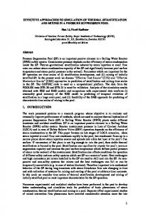
where � (b) is an integer function that has the value 1 if the boolean b is true, and the value 0 otherwise. Thus the function f has the value 1 when access is permitted to the resource and has the value 0 otherwise. Figure 1 provides a graphical illustration of this model. The local transition matrix for automaton A(i) is
Ql i
( )
=
! ?� i f � i f : � i ?� i ( )
( )
10
( )
( )
A(1)
A(N )
sleeping
sleeping
. . .
�(N )
�(1) �(1)f
�(N ) f
. . .
using
using
Figure 1: Resource Sharing Model Note that f depends on the state of other automata, which introduces a functional relation into Q(l i) . The overall descriptor for the model is
Q = �g Ni=1 Q(l i) =
N X i=1
I2 g � � � g I2 g Q(l i) g I2 g � � � g I2 ;
where g denotes the generalized tensor operator, a precise de nition of which is given in Section 7. The SAN product state space for this model is of size 2N . Notice that when P = 1, the reachable state space is of size N +1, which is considerably smaller than the product state space, while when P = N the reachable state space is the entire product state space. Other values of P give rise to intermediate cases.
4.2 A Queueing Network with Blocking and Priority Service
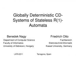
The second model we shall use is an open queueing network of three nite capacity queues and two customer classes. Class 1 customers arrive from the exterior to queue 1 according to a Poisson process with rate �1. Arriving customers are lost if they arrive and nd the bu�er full. Similarly, class 2 customers arrive from outside the network to queue 2, also according to a Poisson process, but this time at rate �2 and they also are lost if the bu�er at queue 2 is full. The servers at queues 1 and 2 provide exponential service at rates �1 and �2 respectively. Customers that have been served at either of these queues try to join queue 3. If queue 3 is full, class 1 customers are blocked (blocking after service) and the server at queue 1 must halt. This server cannot begin to serve another customer until a slot becomes available in the bu�er of queue 3 and the blocked customer is transferred. On the other hand, when a (class 2) customer has been served at queue 2 and nds the bu�er at queue 3 full, that customer is lost. Queue 3 provides exponential service at rate �3 to class 1 customers and at rate �3 to class 2 customers. In queue 3, class 1 customers have preemptive priority over class 2 customers. Customers departing after service at queue 3 leave the network. We shall let Ck ? 1, k = 1; 2; 3 denote the nite bu�er capacity at queue k. Queues 1 and 2 can each be represented by a single automaton (A(1) and A(2) respectively) with a one-to-one correspondance between the number of customers in the queue and the state 1
2
11
of the associated automaton. Queue 3 requires two automata for its representation; the rst, A(3 ), provides the number of class 1 customers and the second, A(3 ), the number of class 2 customers present in queue 3. Figure 2 illustrates this model. 1
2
A(1)
�1
C1 ? 1 loss
1
A(2)
�2
A(3 ) A(3 )
�1
2
C3 ? 1 �31 �32
C2 ? 1 �2
loss
loss
Figure 2: Network of Queues Model This SAN has two synchronizing events: the rst corresponds to the transfer of a class 1 customer from queue 1 to queue 3 and the second, the transfer of a class 2 customer from queue 2 to queue 3. These are synchronizing events since a change of state in automaton A(1) or A(2) occasioned by the departure of a customer, must be synchronized with a corresponding change in automaton A(3 ) or A(3 ), representing the arrival of that customer to queue 3. We shall denote these synchronizing events as s1 and s2 respectively. In addition to these synchronizing events, this SAN required two functions. They are: 1
2
f = �(sA(3 ) + sA(3 ) < C3 ? 1) 1
2
g = �(sA(3 ) = 0) 1
The function f has the value 0 when queue 3 is full and the value 1 otherwise, while the function g has the value 0 when a class 1 customer is present in queue 3, thereby preventing a class 2 customer in this queue from receiving service. It has the value 1 otherwise. Since there are two synchronizing events, each automaton will give rise to ve separate matrices in our representation. For each automaton k we will have a matrix of local transitions, denoted by Q(l k) ; a matrix corresponding to each of the two synchronizing events, Q(sk) and Q(sk), and a diagonal corrector matrix for each synchronizing event, Q� (sk) and Q� (sk) . In these last two matrices, nonzero appear only along the diagonal; they are de ned in such a way � (kelements � � can � ) (k ) � as to make k Qsj + k Qsj ; j = 1; 2, generator matrices (row sums equal to zero). The ve matrices for each of the four automata in this SAN are as follows (where we use Im to denote the identity matrix of order m). 1
1
12
2
2
For A(1):
0 BB B Ql = B BB @ (1)
?� 0 .. . 0 0
... ... ... � � � 0 ?�1 ��� 0 0 00 0 0 B 0 ?�1 0 B B .. . . . . . . (1) Q� s = B . B B @ 0 ��� 0 0 ��� 0 1
For A(2):
0 ?� � BB 0 ?� B .. . . Ql = B . BB . @ 0 ��� 0 ��� 00 B 0 B B B � Qs = B ... B @0 2
2
2
(2)
2
1
Ql
(31 )
0
�2
... 0 0 0
2
0 0 0 0 ��� B 0 ��� � ?� B B . . . .. .. .. ... =B B B @ 0 � � � � ?� 0 ��� 0 � 0f 0 0 B 0 f 0 B B B � Qs = B ... . . . . . . B @ 0 ��� 0 0 ��� 0 31
31
31
31
31
(31 ) 1
For A(3 ) :
.. C ; . C C
0
��� ��� 0
1
��� ��� 0
2
Ql
0 0 .. . 0 0
1 CC CC ; CC A
� (2) Q(2) s : s = IC = Q 2
1
1
2
Qs
(31 ) 1
00 BB 0 B .. =B BB . @0
f
0 ...
��� 0 ���
31
0 ��� 0 f ��� 0 . . . . . . ... 0 0 f 0 0 0
1 CC CC CC ; A
Qs(3 ) = IC = Q� (3s ) : 2
1
3
2
1
0 0
32
32
1 CC CC ; CC A
?� ��� 0 1 � � � 0 CCC . . . ... C CC ; f 0A
32
32
2
0 0 ��� 0 0 ��� 2 ... ... ... � � � �2 0 0 � � � 0 �2
2
1 CC CC CC ; A
0 0 .. . 0
1
2
(2)
?�
1 CC CC CC ; A
� (1) Q(1) s = IC = Q s :
0 0 BB � B .. Qs = B BB . @ 0 0 0 .. . 0
...
?�
.. . 0 0
0 0 .. . 0 0
1
0
0 0 0 0 ��� 0 BB � g ?� g 0 � � � 0 B .. .. ... ... ... =B . BB . @ 0 � � � � g ?� g 0 0 � � � 0 � g ?� 32
?�
2
2
(32 )
1 CC CC CC ; A
0 0 .. . 0
...
?�
�1
1
�1 A
0 0 ��� 0 0 ��� ... ... ... � � � �1 0 � � � 0 �1
0
(1)
��� 0 1 � � � 0 CCC . . . ... C CC ; ?� � A
0 0 ?�2 0 ... ... ��� 0 0 ��� 0
(2)
For A(3 ) :
0 BB B Qs = B BB @
1
�1 0 � � � 0 ?�1 �1 � � � 0 CCC
1
32
0 1?f f 1 BB 0 1 ? f CC B CC ... CC ; Qs = BBB ... @ 0 A ��� 0 ��� g (32 ) 2
13
��� 0 1 f ��� 0 C C . . . . . . ... C CC ; A 0 1?f f C 0
0
0
1
Q� s(3 ) = IC = Qs(3 ) = Q�s(3 ): 2
2
3
1
2
1
2
The overall descriptor for this model is given by
Q = �g Q(l i) + g Q(si) + g Q� (si) + g Q(si) + g Q� (si) ; 1
1
2
2
where the generalized tensor sum and the four generalized tensor products are taken over the index set f1, 2, 31 and 32 g. The reachable state space of the SAN is of size C1 � C2 � C3 (C3 +1)=2 whereas the complete SAN product state space has size C1 � C2 � C32 . Finally, we would like to draw our readers attention to the sparsity of the matrices presented above.
5 Product Forms Stochastic automata networks constitute a general modelling technique and as such they can sometimes inherit results from those already obtained by other modelling approaches. Jackson networks, for example, may be represented by a SAN; the reversibility results of Kelly, [26], and the competition conditions of Boucherie, [6], can be applied to SANs leading to product forms. In this section we shall present su�cient conditions for a SAN to have a product form solution. These conditions extend those given by Boucherie and in addition may be shown to be applicable to truncated state spaces. They apply only to SANs with no synchronizing events, which means that the transitions of the SAN can only be transitions of one automaton at a time. Thus Jackson networks lie outside their scope of applicability. The way we proceed is to work on global balance equations and search for su�cient conditions on the functional transition rates to obtain a product form solution. Let us state the problem more formally. Consider a SAN with N automata and local transition matrices Q(l k), k = 1; 2; : : :; N . The states of A(k) are denoted ik 2 S (k), and a state of the SAN is denoted i = (i1; :::; iN ). A state of the SAN without automaton A(k) is denoted i�k = (i1; :::; ik?1; ik+1 ; :::; iN ). A state i in which the kth component is replaced by i0k is denoted by i�k ji0k . For ik 6= i0k , the elements of Q(l k) are assumed to be of the following form
Q(l k) (ik ; i0k ) = q (k) (ik ; i0k)f (k) (i; i0); where q (k) (ik ; i0k ) is a constant transition rate and f (k) (i; i0) is any positive function. Notice that when the transition of the SAN is occasioned by a transition of its kth automaton, the function f (k) (i; i0) actually depends only on i and i0k . Assume now that the q (k) (ik ; i0k ) satisfy balance equations in the sense that there exist a set of positive numbers � (k)(ik ) which sum to 1 and which satisfy either local balance equations within each automaton
8ik ; i0k 2 S k ; � k (ik )q k (ik ; i0k) = � k (i0k)q k (i0k ; ik); ( )
( )
( )
or a global balance equation for each automaton
8ik 2 S k ; ( )
X �
i0k 2S (k)
( )
( )
�
�(k)(ik )q (k) (ik ; i0k) ? � (k)(i0k )q (k)(i0k ; ik ) = 0:
14
(8) (9)
Note that equation (8) is stronger, and implies, equation (9). The SAN generator is Q = �Nk=1 Q(l k). Its transition rates, for i 6= i0, are given by
q(i; i0) =
(
q (k) (ik ; i0k )f (k)(i; i�k ji0k ) 0
if i0 = i�k ji0k otherwise
The reachable state space of the SAN is denoted byQR and, because of the e�ect of functional transitional rates, can be strictly smaller that S = N1 S (k). The global balance equations for the SAN are, for i 2 R, X? � �(i)q(i; i0) ? �(i0)q(i0; i) = 0: (10) Substituting
i0 2S for q (i; i0) and q (i0; i) in
(10) yields
N X � X
�
k=1 i0k 2S (k)
�(i)q (k)(ik ; i0k )f (k)(i; i�kji0k ) ? �(i�k ji0k )q (k) (i0k ; ik )f (k)(i�k ji0k ; i) = 0:
(11)
Q This SAN has a product form solution if, for some normalizing constant C , � (i) = C N1 � (k) (ik ) is a solution of these balance equations. Substituting this into (11) gives N Y N X k=1 j =1;j 6=k
�(j) (ij )
N � X i0k 2S (k)
�
� (k)(ik )q (k)(ik ; i0k )f (k) (i; i�kji0k ) ? � (k)(i0k )q (k)(i0k ; ik )f (k) (i�k ji0k ; i) = 0:
Now it only remains to nd su�cient conditions on the functions f (k) for which N � X i0k 2S (k)
�(k)(ik )q (k)(ik ; i0k )f (k) (i; i�kji0k ) ? � (k)(i0k )q (k) (i0k ; ik )f (k) (i�k ji0k ; i)
�
(12)
is equal to zero, knowing the balance equations, (8) or (9).
First case: The set of balance equations (8) is satis ed and the functions f k express a ( )
truncation of the state space of the SAN (similar to that described by Kelly). That is to say, the functions are equal to the indicator function of the reachable state space R: f (k) (i; i0) = � (i; i0 2 R). Thus the expression (12) is trivially equal to zero: either i�k ji0k 2 R (the functions are equal to 1) and we have the local balance equations, or i�k jPi0k 2= R Q and the functions themselves are zero. The normalizing constant C is the inverse of i2R Nk=1 � (i) and might be di�cult to compute if R is large.
Second case: The set of balance equations (9) is satis ed and the functions f k depend ( )
only on i�k and not on the current state of automaton k. This means that the decomposition Q(l k) (ik ; i0k) = q (k)(ik ; i0k)f (k) (i; i0) is a real product form. The variable q (k) (ik ; i0k ) is the local transition rate of automaton k and f (k) (i; i0) = f (k)(i�k ) expresses the interaction of the rest of the SAN when it is in state i�k . In essence, the functions f (k) (i�k ) either force the system to halt, if they evaluate to zero (| This can also be interpreted as a truncation of the state space), or else permit the automaton A(k) to execute independently, albeit with modi ed rates: the 15
function uniformly slows down or speeds up the automaton for a given i�k . When i�k changes, the slowing/speeding factor changes. The balance equations are given by
f (k) (i�k )
N Y j =1;j 6=k
�(j) (ij )
X � i0k 2S (k)
�
�(k)(ik )q (k)(ik ; i0k ) ? � (k) (i0k )q (k) (i0k ; ik ) = 0
which must hold because the local balance equations themselves, (9), hold. This second case is a generalization of the Boucherie competition conditions. The constant C is equal to 1 when the reachability space is the product space; otherwise it must be chosen so that the individual probabilities sum to one.
Third case: Notice that the two previous cases are not overlapping, and this for two reasons: � In case 1, f k (i; i0) = �(i; i0 2 R) which reduces to �(i�k ji0k 2 R) for each balance equation (8). In general, the function � (i�k ji0k 2 R) depends not only on i�k , but on i0k as well. � In case 2, we have a \uniform" modi cation of the rates of A k while in case 1, they are ( )
( )
either 0 or unchanged, for a given i�k . This presents the possibility of combining cases 1 and 2 to yield a third case: f (k) (i; i0) = �(i; i0 2 R)f (k)(i�k ):
Using the notation described above, we may summarize these results in the following theorem:
Theorem 5.1 Given a SAN having no synchronizing events and in which the elements of Ql k are of product form type; i.e., for ik = 6 i0k ,
( )
Q(l k) (ik ; i0k ) = q (k) (ik; i0k )f (k) (i; i0);
Q each of the following su�cient conditions leads to a product form solution, � (i) = C N1 � (k) (ik ): � Case 1: f (k)(i; i0) = �(i; i0 2 R) � Case 2: f (k)(i; i0) = f (k) (i�k) � Case 3:
f (k)(i; i0) = �(i; i0 2 R)f (k)(i�k )
The � (i) satisfy the global balance equations for the SAN, C is a normalizing constant and the �(k) (ik ) are solutions of the local balance equations (8) for cases 1 and 3 and a solution of (9) for case 2.
Examples: 1. The resource sharing example of Section 4.1 falls into case 2 with
0 N 1 0 N 1 X X f k (i; i0) = � @ �(ij = using) < P A = � @ �(i0j = using) < P A : ( )
j =1;j 6=k
j =1;j 6=k
16
2. Consider a number, N , of identical processes each represented by a three state automaton. State 1 represents the state in which the process computes independently; state 2 represents an interacting state (int) in which the automaton computes and sends messages to the other automata and state 3 is a state in which the process has exclusive access in order to write (w) to a critical resource. Each process may move from any of the three states to any other according to well de ned rates of transition. To provide for mutually exclusive access to the critical resource, the rates of transition to state 3 must be multiplied by a function g de ned as 0 N 1 X g (k)(i; i0) = � @ �(ij = w) = 0A : j =1;j 6=k
To provide for the e�ect of communication overhead, all transition rates within the automaton k; k = 1; 2; : : :; N must be multiplied by a function f (k) de ned as
C : j =1;k6=j � (ij = int)
f (k) (i; i0) = PN
Such a SAN therefore falls into case 2, too. 3. The examples provided in the paper of Boucherie, [6]; viz: the dining philosophers problem, locking in a database system, and so on, all fall into case 2. In these examples, the functions f (k) (i�k ) express a reachable state space and yield a uniform multiplicative factor. Other examples may be found in [14, 19, 22, 28]. 4. Our nal example explicitly displays the dependence of the function on i0 and falls into case 1. Consider a system consisting of P units of resource and N identical processes, each represented by a three-state Markov chain. While in state 0, a process may be considered to be sleeping; in state 1, it uses a single unit of resource; while in state 2, the process uses 2 units of the resource. The transitions among its three states are such that while in the sleeping state (0), it can move directly to either state 1 or 2, (i.e., it may request, and receive, a single unit of resource, or two units of resource). From state 2, the process can move to state 1 or to state 0, (i.e., it may release one or both units of the resource). Finally, from state 1, it can move to state 0 or to state 2 (i.e., with a single unit of resource, it has the choice of releasing this unit or acquiring a second). To cater for the case in which su�cient resources are not available, the rates of transition towards states 1 and 2 must each be multiplied by the function
0 1 N X f k (i; i0k) = � @(i0k + ij ) � P A : ( )
j =1
For certain values of the transition rates, (e.g., q (0; 1) = q (1; 2); q (2; 1) = q (1; 0) and q(0; 2) = q(2; 0)), there exists a solution to the balance equations (8) and the SAN has product form.
6 Vector-Descriptor Multiplications Typically, product form solutions are not available and the analyst must turn to other solutions procedures. When the global in nitesimal generator of a SAN is available only in the form of a 17
SAN descriptor, the most general and suitable methods for obtaining probability distributions are numerical iterative methods, [44]. Thus, the underlying operation, whether we wish to compute the stationary distribution, or the transient solution at any time t, is the product of a vector with a matrix. Since
xQ = x
EXN
2 +
j =1
Ni Qji = ( )
=1
the basic operation is
EXN
2 +
j =1
x Ni=1 Q(ji);
x Ni=1 Q(i)
where, for notational convenience, we have removed the subscripts on the Q(ji) . It is essential that this operation be implemented as e�ciently as possible. The following theorem is proven in [33]. Theorem 6.1 The product
x Ni=1 Q(i) ;
Q where Q(i), of order ni , contains only constant terms and x is a real vector of length Ni=1 ni , may be computed in �N multiplications, where �N = nN � (�N ?1 +
N Y i=1
ni ) =
N Y i=1
ni �
N X i=1
ni ;
�0 = 0:
To compare this with the number needed when advantage is not taken of the special� structure �2 Q resulting from the tensor product, observe that to naively expand Ni=1 Q(i) requires Ni=1 ni � � multiplications and that this same number is required each time we form the product x Ni=1 Q(i) . It is important to note however, that this complexity result is valid only when the stochastic automata contain non-functional rates. A proof is given in [33]. An example will help us see this more clearly and at the same time show us where extra multiplications are needed for functional transitions. Consider two stochastic automata, the rst A with n1 = 2 states and the second B with n2 = 3 states, (as in equation (3)). The product y = x(A B) may be obtained as
y1 = a11(x1 b11 + x1 b21 + x1 b31) + a21(x2 b11 + x2 b21 + x2 b31) y1 = a11(x1 b12 + x1 b22 + x1 b32) + a21(x2 b12 + x2 b22 + x2 b32) y1 = a11(x1 b13 + x1 b23 + x1 b33) + a21(x2 b13 + x2 b23 + x2 b33) 1
1
2
1
3
2
3
2
1
2
3
1
2
3
3
1
2
3
1
2
3
(13)
y2 = a12(x1 b11 + x1 b21 + x1 b31) + a22(x2 b11 + x2 b21 + x2 b31) y2 = a12(x1 b12 + x1 b22 + x1 b32) + a22(x2 b12 + x2 b22 + x2 b32) y2 = a12(x1 b13 + x1 b23 + x1 b33) + a22(x2 b13 + x2 b23 + x2 b33) 1
1
2
3
1
2
3
2
1
2
3
1
2
3
3
1
2
3
1
2
3
Note that each inner product (within the parentheses) above the horizontal line is also to be found below the line and so each needs to be computed only once. Since there are n1 n2 such inner products, and since each involves n2 multiplications, the total number of multiplications needed to evaluate them is n1 n22 . Also, each of the n1 n2 inner products is multiplied by n1 18
di�erent elements of the matrix A. The total number of multiplications needed to compute the product y = x(A B ) is thus n22 n1 + n2 n21 = n1 n2 (n1 + n2 ). Let us now examine the e�ect of introducing functional rates. The savings made in the computation of x Ni=1 Q(i) are due to the fact that once a product is formed, it may be used in several places without having to re-do the multiplication. Even with functional rates, which imply that the elements in the matrices change according to their context, this same savings is sometimes possible [44]. This leads to an extension of some of the properties of tensor products and to the concept of Generalized Tensor Products (GTPs) as opposed to Ordinary Tensor Products (OTP).
7 Generalized Tensor Products
We assume throughout that all matrices are square. We shall use B [A] to indicate that the matrix B may contain transitions that are a function of the state of the automaton A. More generally, A(m) [A(1); A(2); : : :; A(m?1) ] indicates that the matrix A(m) may contain elements that are a function of one or more of the states of the automata A(1); A(2); : : :; A(m?1). We shall use the notation g to denote a generalized tensor product. Thus A g B [A] denotes the generalized tensor product of the matrix A with the functional matrix B [A] and we have 0 1 a11B(a1 ) a12B(a1 ) � � � a1na B(a1 ) BB a21B(a2 ) a22B(a2) � � � a2na B(a2) CC CC ; A g B[A] = B (14) .. .. .. ... B@ . . . A ana 1B(ana ) ana 2 B(ana ) � � � ana na B(ana ) where B (ak ) represents the matrix B when its functional entries are evaluated with the argument ak ; k = 1; 2; : : :; na, the ai being the states of automaton A. Also, 0 1 a11[B]Inb � B a12[B]Inb � B � � � a1na [B]Inb � B BB a21[B]Inb � B a22[B]Inb � B � � � a2na [B]Inb � B CC CC ; A[B] g B = B .. .. .. ... B@ . . . A ana1 [B]Inb � B ana 2[B]Inb � B � � � ana na [B]Inb � B where aij [B]Inb = diagfaij(b1); aij (b2); : : :; aij (bnb )g and aij (bk ) is the value of the ij th element of the matrix A when its functional entries are evaluated with the argument bk ; k = 1; 2; : : :; nb. Finally, when both automata are functional we have 0 1 a11 [B]Inb � B(a1 ) a12[B]Inb � B(a1 ) � � � a1na [B]Inb � B(a1 ) BB a21[B]Inb � B(a2) a22[B]Inb � B(a2 ) � � � a2na [B]Inb � B(a2) CC CC : A[B] g B[A] = B .. .. .. . B@ . . . . . A ana 1[B]Inb � B(ana ) ana 2 [B]Inb � B(ana ) � � � ana na [B]Inb � B(ana ) For A[B] g B [A], the generic entry (l; k) within block (i; j ) is aij (bk ) � bkl (ai ). We now present a number of lemmas concerning generalized tensor products. Their proofs may be found in [15]. These lemmas are useful for deriving many important properties of generalized tensor products. 19
Lemma 7.1 (GTP: Associativity) (A[B; C ] g B [A; C ]) g C [A; B] = A[B; C ] g (B [A; C ] g C [A; B]) Lemma 7.2 (GTP: Distributivity over Addition) (A [B] + A [B]) g (B [A] + B [A]) = (A [B] g B [A] + A [B] g B [A] + A [B] g B [A] + A [B] g B [A]) 1
1
1
2
1
1
2
2
2
1
1
2
As for ordinary tensor products, compatibility with multiplication usually does not hold for generalized tensor products either. However, there exists three degenerate compatibility forms when some of the factors are identity matrices and not all of the factors have functional entries. They are
Lemma 7.3 (GTP: Compatibility over Multiplication: I | Two Factors) (A[C ] � B [C ]) g Inc = (A[C ] g Inc ) � (B [C ] g Inc ) Similarly,
Inc g (A[C ] � B[C ]) = (Inc g A[C ]) � (Inc g B[C ]):
Lemma 7.4 (GTP: Compatibility over Multiplication: II | Two Factors) A g B[A] = [A � Ina ] g [Inb � B[A]] = (Ina g B[A]) � (A Inb ) : Lemma 7.5 (GTP: Compatibility over Multiplication: III | Two Factors) A[B] g B = [A[B] � Ina ] g [Inb � B] = (A[B] g Inb ) � (Ina B) : This lemma still holds if Ina is replaced by any constant matrix. In the following lemmas, if Q k ni is the size of matrix Ai , then Il:k denotes the identity matrix of size i=l ni.
Lemma 7.6 (GTP: Compatibility over Multiplication | Many Factors) A g A [A ] g A [A ; A ] g � � � g A m [A ; : : :; A m? ] = I m? g A m [A ; : : :; A m? ] � I m? g A m? [A ; : : :; A m? ] g Im m � ��� � I g A [A ] g I m � A g I m (1)
(2)
(1)
(3)
(1)
(2)
1:
1
1:
2
1:1
(1)
(
(
(
(2)
)
(1)
1)
3:
2:
20
(1)
(
(
(1)
(1)
)
1)
1)
(
2)
:
(15)
Similarly, one may use Lemma 7.5 to nd
A(m) [A(1); : : :; A(m?1)] g A(m?1) [A(1); : : :; A(m?2) ] g � � � g A(2)[A(1)] g A(1) = A(m) [A(1); : : :; A(m?1)] g Im?1:1 � Im:m g A(m?1)[A(1); : : :; A(m?2)] g Im?2:1
� ��� � Im g A [A ] g I � Im g A (2)
:3
(1)
1:1
(16)
(1)
:2
In Lemma 7.6, only one automaton can depend on all the (m ? 1) other automata, only one can depend on at most (m ? 2) other automata and so on. One automaton must be independent of all the others. This provides a means by which the individual factors on the left-hand side of equation (15) may be ranked; i.e., according to the number of automata on which they may depend. An automaton may actually depend on a subset of the automata in its parameter list.
Lemma 7.7 (GTP: Pseudo-Commutativity) Let � be a permutation of the integers [1; 2; : : :; N ], then there exists a permutation matrix, P� of order QNi=1 ni , such that
g Nk A k [A ; : : :; A N ] = P� g Nk A � k [A ; : : :; A N ]P�T : =1
( )
(1)
(
)
=1
( ( ))
(1)
(
)
These lemmas allow the following theorem to be proven. (The proof itself may be found in [15].)
Theorem 7.1 (GTP: Algorithm) The multiplication � � x � A g A [A ] g A [A ; A ] g � � � g A N [A ; : : :; A N ? ] Q where x is a real vector of length N n may be computed in O(� ) multiplications, where (1)
(2)
(1)
(3)
i=1 i N Y
�N = nN � (�N ?1 +
i=1
(1)
(2)
(
)
(1)
(
1)
N
ni ) =
N Y i=1
ni �
N X i=1
ni ;
�0 = 0:
with the algorithm described in Figure 3.
The following algorithm is based directly on Lemma 7.6 and implements an e�cient product of a vector x with a generalized tensor product in which the automata satisfy the functional (i?1) dependencies described in Lemma 7.6. In this algorithm, the notation A(i) [a(1) k ; : : :; aki? ] implies that the matrix is evaluated under the assumption that automaton A(j ) is in state a(kjj) , for j = 1; 2; : : :; i ? 1. The cost of the function evaluations is included in the de nition of the big Oh formula. We would like to point out that although Lemma 7.7 allows us to reorganize the terms in the generalized tensor product in any way we wish, the advantage of leaving them in the form given above is precisely that the computation of the state indices, kj , can be moved outside the innermost summation of the algorithm. 1
21
1
Figure 3: Algorithm for Vector Multiplication with a Generalized Tensor Product � � x A g A [A ] g A [A ; A ] g � � � g A N [A ; : : :; A N ? ] (1)
(2)
(1)
(3)
(1)
(2)
(
)
(1)
(
1)
1. Initialize: nleft = n1 n2 � � � nN ?1 ; nright = 1. 2. For i = N; : : :; 2; 1 do � base = 0; jump = ni � nright � For k = 1; 2; : : :; nleft do � For j = 1�h ; 2; : : :; i ? 1 do i �� � � kj = (k ? 1)= Qil=?j1+1 nl mod Qil=?j1 nl + 1 � For j = 1; 2; : : :; nright do � index = base + j � For l = 1; 2; : : :; ni do � zl = xindex ; index = index + nright (i?1) � Multiply: z0 = z � A(i)[a(1) k ; : : :; aki? ] � index = base + j � For l = 1; 2; : : :; ni do � xindex = zl0; index = index + nright � base = base + jump � nleft = nleft=ni?1 � nright = nright � ni 1
1
Proof: Observe that the inner-most loop (which is in fact implicitly rather than explicitly
de ned in the algorithm by the call to the function Multiply) involves computing the product of a vector z , of length ni , with a matrix of size ni � ni . This requires (ni )2 multiplications, assuming that the matrices are full. This operation lies within consecutively nested i, k and j Q N loops, Since the k and j loops together involve l=1 nl =ni iterations, and the outermost i loop is executed N times, the total operation count is given by N QN n ! N N X l n = Yn �Xn : l i i i n =1
i=1
i
2
i=1
i=1
2
The complexity result of Theorem 7.1 was computed under the assumption that the matrices are full. However, the number of multiplications may be reduced by taking advantage of the fact that the block matrices are generally sparse. It is immediately apparent that when the matrices are not full, but possess a special structure such as tridiagonal, or contain only one nonzero row or column, etc., or are sparse, then this may be taken into account and this number reduced in consequence. To see how sparsity in the matrices Q(i) may be taken into account let us denote by zi the number of nonzero entries in Q(i). Then the multiply operation of the previous algorithm, i.e., the operation inherent in the statement 22
* Multiply: z 0 = z � Q(i) , has complexity of order zi , so, taking the nested loops into account, the overall operation has a complexity of the order of N N N X N X Y Y zi ni = ni zj : i=1
i=1;i6=j
i=1
j =1 nj
To compare this complexity with a global sparse format, the number of nonzero entries of Q Q P N N N It is hard in general to compare the two numbers i=1 zi and i=1 ni j =1 nzjj . Note however that if all zi = N 1=(N ?1)ni , both orders of complexity are equal. If all matrices are sparse (e.g., below this bound), the sparse method is probably better in terms of computation time. This remark is valid for a single tensor product. For a descriptor which is a sum of tensor products and where functions in the matrices Q(i) may evaluate to zero, it is hard to compute, a priori, the order of complexity of each operation. In this case, insight can only be obtained from numerical experiments.
Ni=1 Q(i) is QNi=1 zi.
We now introduce one nal lemma that allows us to prove a theorem (Theorem 7.2) concerning the reduction in the cost of a vector-descriptor multiplication in the case when the functional dependencies among the automata do not satisfy the constraints given above. Lemma 7.8 (GTP: Decomposability into OTP) Let `k (A) denote the matrix obtained by setting all elements of A to zero except those that lie on the kth row which are left unchanged. Then na X A g B[A] = `k (A) B[ak ]: k=1
Thus we may write a generalized tensor product as a sum of ordinary tensor products. A term g Ni=1 A(i)[A(1); : : :; A(N )] involved in the descriptor of a SAN is said to contain a functional dependency cycle if it contains a subset of automata A(p); A(p+1); : : :; A(p+c) , c � 1, with the property that the matrix representation of A(p+i) contains transitions that are a function of A(p+(i+1)modc ) , for 0 � i � c. For example, a SAN with two automata A and B contains a term with a functional dependency cycle if and only if the matrix representations are such that A is a function of B, (A[B]), B is a function of A, (B [A]), and A[B] B [A] occurs in the descriptor. Let G denote a graph whose nodes are the individual automata of a SAN and whose arcs represent dependencies among the automata within a term of the descriptor. Let T be a cutset of the cycles of G , [5]. Then T is a set of nodes of G with the property that G ? T does not contain a cycle where G ? T is the graph of G with all arcs that lead into the nodes of T removed. +1
Theorem 7.2 (GTP with Cycles: Complexity of Vector-Descriptor Product)
Given a SAN descriptor containing a term with a functional dependency graph G and cutset T of size t, the cost of performing the vector-descriptor product x � g Ni=1 A(i)[A(1); : : :; A(N )] is 0 1 1 !0 N N N @ Y ni A Y ni @ X ni A : i=1;i2T
i=1
23
i=1;i62T
8 Applicability of the Multiplication Theorems We now return to the context of SANs proper. We have seen that the descriptor of a SAN is a sum of tensor products and we now wish to examine each of the terms of these tensor products in detail to see whether they fall into the categories of Theorem 7.1 or 7.2. In the case of SANs in continuous-time, and with no synchronized transitions, the descriptor is given by
Q = �g Nk=1 Q(k) =
N X k=1
In g � � � g Ink? g Q(k) g Ink g � � � g InN ; 1
1
+1
and we can apply Theorem 7.1 directly to each term of the summation. Notice that all but one of the terms in each tensor product is an identity matrix, and as we pointed out in the proof of Theorem 7.1, advantage can be taken of this to reduce the number of multiplications involved. Consider now what happens when we add synchronizing events. The part of the SAN descriptor that corresponds to local transitions has the same minimal cost as above which means that we need only consider that part which is speci cally involved with the synchronizing events. Recall from Section 3.3, that each synchronizing event results in an additional two terms in the SAN descriptor. The rst of these may be thought of as representing the actual transitions and their rates; the second corresponds to an updating of the diagonal elements in the in nitesimal generator to re ect these transitions. Since the second is more e�ciently handled separately and independently, we need only be concerned with the rst. It can be written as
Ni Qji : =1
( )
We must now analyze the matrices that represent the di�erent automata in this tensor product. There are three possibilities depending upon whether they are una�ected by the transition, are the designated automaton with which the transition rate of the synchronizing event is associated, or are a�ected in some other manner by the event. These matrices have the following structure.
� Matrices Qji corresponding to automata that do not participate in the synchronizing event ( )
are identity matrices of appropriate dimension. � With each synchronizing event is associated a particular automaton. In a certain sense, this automaton may be considered to be the owner of the synchronizing event. We shall let E denote the matrix of transition rates associated with this automaton. For example, if a synchronizing event e arises as a result of the automaton changing from state i to state j , then the matrix E consists entirely of zeros with a single nonzero element in position ij . This nonzero element gives the rate at which the transition occurs. If several of the elements are nonzero, this indicates that the automaton may cause this same synchronizing event by transitions from and to several states. � The remaining matrices correspond to automata that are otherwise a�ected by the synchronizing event. We shall refer to these as � matrices. Each of these � matrices consists of rows whose nonzero elements are positive and sum to 1 (essentially, they correspond to routing probabilities, not transition rates), or rows whose elements are all equal to zero. The rst case corresponds to the automaton being synchronized into di�erent states according to certain xed probabilities and the state currently occupied by the automaton. In the second case, a row of zeros indicates that this automaton disables the synchronized 24
transition while it is in the state corresponding to the row of zeros. In many cases, these matrices will have a very distinctive structure, such as a column of ones, the case when the automaton is forced into a particular state, independent of its current state. When the only functional rates are those of the synchronizing event, only the elements of the matrix E are functional; the other matrices consist of identity matrices or constant � matrices. Thus, once again, this case falls into the scope of Theorem 7.1. This leaves the case in which the � matrices contain transition probabilities that are functional. If there is no cycle in the functional dependency graph then we can apply Theorem 7.1; otherwise we must resort to Theorem 7.2. Notice that if the functional dependency graph is fully connected, Theorem 7.2 o�ers no savings compared with ordinary multiplication. This shows that Theorem 7.2 is only needed when the routing probabilities associated with a synchronizing event are functional and result in cycles within the functional dependency graph, (which we suspect to be rather rare). For SANs in discrete-time, [32], it seems that we may not be so fortunate since cycles in the functional dependency graph of the tensor product tend to occur rather more often. Following up on these results, extensive experiments conducted on a set of small examples, and reported in [16], provided a rule of thumb for ordering automata in a network to achieve better performance. More precisely, it is not the automata in the SAN that must be ordered, but rather, within each term of the descriptor, a best ordering should be computed independently.
9 The Memory versus CPU-time Trade-o� An important advantage that the SAN approach has over others that generate and manipulate the entire state space of the underlying Markov chain is that of minimal memory requirements. The infamous state-space explosion problem associated with these other approaches is avoided. The price to be paid of course, is that of increased CPU time. The obvious question that should be asked is whether some sort of compromise can be reached. Such a compromise would take the form of reducing a SAN with a certain (possibly large) number of \natural" automata each with only a small number of states, to an \equivalent" SAN with less automata in which many (possibly all) have a larger number of states. A natural way to produce such an equivalent SAN is to collect subsets of the original automata into a small number of groups. The limit of this process is a single automaton containing all the states of the Markov chain. However we do not wish to go to this extreme. Observe that just four automata each of order 100 brings us to the limit of what is currently possible to solve using regular sparse matrix techniques yet memory requirements for four automata of size 100 remain modest. Furthermore, in the process of grouping automata, a number of simpli cations may result. For example, automata may be grouped in such a way that some (or all) of the sychronizing events disappear, or grouped so that functional transition rates become constant, or both. Furthermore, it is frequently the case that the reachable state space of the grouped automata is smaller than the product state space of the automata that constitute the group. To pursue this line of thought, we shall need to de ne our notion of equivalence among SANs and the grouping process. Consider a SAN containing N stochastic automata A1 ; : : :; AN of size ni respectively, E synchronizing events s1 ; : : :; sE , and functional transition rates. Its descriptor may be written
25
as
Q=
NX +2E
Ng;i Qji : ( )
j =1
=1
Let 1; : : :; N be partitioned in B groups called b1; : : :; bB , and, without loss of generality, assume that b1 = [1; : : :; c2], b2 = [c2 + 1; : : :; c3], etc, for some increasing sequence of ci, with c1 = 0, cB+1 = N . The descriptor can be rewritten, using the associativity of the generalized tensor product, as 2E +N � � X
Bg;k=1 cg;jk =ck +1 Q(ji) : Q= +1
j =1 Q(ji), for
cg;jk+1=ck +1
The matrices R(jk) = j 2 1; : : :; 2E + NQ, are, by de nition, the transition matrices of a grouped automaton, called Gk of size hk = ci=k ck +1 ni . The descriptor may be rewritten as 2E +N X Q=
Bg;k=1 R(jk): +1
j =1
Separating out the terms resulting from local transitions from those resulting from synchronizing events, we obtain
Q=
NX +2E j =1
Ng;i Qji = �Ng;i Ql i + =1
( )
=1
( )
E � X j =1
�
Ng;i Qsij + Ng;i Q� sij : =1
( )
( )
=1
Grouping by associativity gives
Q = �Bg;k=1 R(l k) + with
E � X j =1
�
Bg;k Rskj + Bg;k R�skj ; =1
( )
=1
R� (skj ) = cg;ik =ck +1 Q� (sij) :
R(skj ) = cg;ik =ck +1 Q(sij) ;
R(l k) = �cg;ik =ck +1 Q(l i) ;
+1
+1
+1
( )
First simpli cation: Removal of synchronizing events. Assume that one of the synchronizing events, say s1 , is such that it synchronizes automata within a group, say b1. As a result, this synchronizing event becomes internal to group b1 and may be treated as a transition that is local to G1 . In this case, the value of R(1) l may be changed in order to simplify the formula for the descriptor. Using (1) (1) � (1) R(1) s ; l (= Rl + Rs + R 1
1
the descriptor may be rewritten as
�Bg;k Rl k + =1
( )
E � � X
Bg;i Rsij + Bg;i R�sij : j =2
=1
( )
=1
( )
The descriptor is thus reduced (two terms having disappeared). This procedure can be applied to all identical situations. 26
Second simpli cation: Removal of functional terms. Assume now that the local transition matrix of G1 is a tensor sum of matrices whose elements are functions only of the states of the automata that are in the subset b1 . Then the functions in Q(l i) of (i) c R(1) l = �g;i=c +1 Ql 2
1
may be evaluated when performing the generalized tensor operator and R(1) l becomes a constant matrix. As for the removal of synchronizing events, this process of replacing functions with constants may be applied in all similar situations. However, if R(1) sj is the tensor product of matrices that are functions of the states of automata, some of which are in b1 and some of which are not in b1, then performing the generalized (i) tensor product R(1) sj = cg;i=c +1 Qsj allows us to only partially evaluate the functions for the arguments in b1. Others arguments cannot be evaluated. These must be evaluated later when performing the computation Bg;i=1 R(sij) and may in fact, result in an increased number of function evaluations. 2
1
Third simpli cation: Reduction of the reachable state space. In the process of grouping, the situation might arise Q that a grouped automata Gi has a reachable state space smaller than the product state space, ci=j cj +1 ni . This happens after simpli cations of type 1 or 2 have been performed. For example, functions may evaluate to zero, or synchronizing events may disable certain transitions. In this case, a reachability analysis may be performed in order to compute the reachable state space. In the SAN methodology, the global reachable state space is known in advance and the reachable state space of a group may be computed by means of a simple projection. +1
A series of numerical experiments conducted on the two examples presented in Section 4 was reported in [16] and quantity the e�ect of these simpli cations. The goal was to observe the e�ect on the time required to perform 10 premultiplications of the descriptor by a vector and on the amount of array storage needed. In the rst model, that of resource sharing, the parameters P and N were varied and the automata (recall that all are identical) were grouped in a variety of ways. The results showed a substantial reduction in CPU time as the number of blocks of automata was reduced, | a combined e�ect of a reduction in the reachable state space, algorithm overhead, and the number of functions that needed to be evaluated, and this with relatively little impact on memory requirements. As concerns memory requirements, two contrasting e�ects were observed. On the one hand, the reduction in the reachable state space caused a subsequent reduction in the size of the probability vectors and hence an overall reduction in the amount of memory needed. On the other hand, the size of the matrices representing the grouped automata increased thereby increasing the amount of memory needed. This latter e�ect was observed to become more important as the number of resources (P ) approached the number of processes (N ) and indeed became the dominant e�ect. The queueing network model was also analyzed under a variety of di�erent parameter values and with two di�erent kinds of grouping: � A grouping of the automata according to customer class (A1 and A3 ) and (A2 and A3 ). 1
27
2
� A grouping of the automata according to queue (A and A ) and (A and A ); 1
2
31
32
The results showed that the CPU times obtained with the rst grouping was worse than in the non-grouped case. This is a result of the fact that this model incorporates functions that cannot be removed using simpli cation 2. Although the rst grouping eliminates the synchronizing events, it results in an increase in the number of functions that must be evaluated and increases the overall time needed. The second grouping allowed for the possibility of a reduction in the state space of the joint automata, (A3 and A3 ), since the priority queue is now represented by a single automaton. This, along with the elimination of functional elements from the grouped descriptors, lead to a reduction in CPU-time. Additionally, the elimination of non-reachable states reduced the amount of array storage needed so that this grouping lead to a reduction in CPU-time and memory needs. This series of experiments showed that the bene ts that accrue from grouping are nonnegligible, so long as the number of function evaluations do not rise drastically as a result. In fact, it seems that function evaluations should be the main concern in choosing which automata to group together. Indirectly, functions also play an important role in identifying non-reachable states, the elimination of which permit important reductions in CPU time and memory. The number of groups should be kept small. Four or less appeared to be optimal in this particular set of experiments. 1
2
10 Numerical Solution Methods Consider a stochastic automata network consisting of N automata. Let Q be its descriptor, i.e.,
Q=
EXN
2 +
j =1
Ni Qji : =1
( )
Our goal is to nd the stationary probability vector, i.e., a vector � such that �Q = 0 and �e = 1. (See also Chapter 3.) Of all the numerical solution methods discussed in [42], only those whose interaction with the in nitesimal generator is its product with a vector, are suitable when the coe�cient matrix is given in this form. Thus, the power method and the various projection methods are easy to implement. It is not easy to see how methods such as Gaussian elimination can be adopted to e�ciently solve SANs. Furthermore, as we have already seen in this chapter, current research has lead to e�cient descriptor-vector multiplication algorithms. The simplest numerical solution method in our context is the power method. If P is the stochastic transition probablity matrix of an irreducible Markov chain, the power method is described by the iterative procedure �(k+1) = � (k) P; (17) where � (0) is an arbitrary initial approximation to the solution. When an in nitesimal generator Q, is available, P may be obtained from P = I + �tQ (18) where �t � 1= maxi jqii j. P may be written as a sum of tensor products, since
I + �tQ = Ni+1 Ini + 28
EXN
2 +
j =1
�t Ni=1 Q(ji):
Thus the power method becomes
�
l
( +1)
0E N 1 X = � l (I + �tQ) = � l + �t� l @
Ni Qji A : ()
()
()
2 +
=1
j =1
(19)
( )
This is the form that the power method takes when it is applied to a SAN descriptor. Projection Methods include the class of methods known as simultaneous iteration or subspace iteration, [25, 41, 45], which iterate continuously with a xed number of vectors, as well as methods that begin with a single vector and construct a subspace one vector at a time, [36]. The subspace most often used in Markov chain problems is the Krylov subspace given by
Km(P; v) = spanfv; vP; vP ; : : :; vP m? g: 2
1
This subspace is spanned by consecutive iterates of the power method and these vectors may be evaluated using (19). Furthermore it is the only part of the projection methods that interacts directly with the coe�cient matrix. It is well known that the projection methods, (and the power method) perform best when accompanied with an e�ective preconditioner. The objective of preconditioning is to modify the eigenvalue distribution of the iteration matrix so that convergence onto the solution vector may be attained more quickly. In a Markov chain context, this usually implies nding a matrix M ?1 so that I ? (I ? P )M ?1 possesses one unit eigenvalue and n ? 1 others that are close to zero. The preconditioned power method is written as �(l+1) = � (l)(I ? (I ? P )M ?1 ) = � (l) ? � (l)(I ? P )M ?1 : (20) The problem is now one of nding a suitable matrix M ?1 . One possibility is to approximate the inverse of I ? P directly by a polynomial series. It is known that, for any matrix A for which kAk � 1, the inverse of I ? A may be written in a Neumann series as, ([20]): (I ? A)?1 =
1 X
k=0
Ak :
Since P is a stochastic matrix, kP k � 1, and so an approximate inverse of ?�tQ = I ? P is given by K X M ?1 = P k : k=0
When this is substituted into equation (20), it gives
�
l
( +1)
l
= � + �t� ()
lQ
()
! K X k k=0
P
:
Since Q and P may be expressed as a sum of tensor products, all numerical operations may be carried out without having to expand the descriptor of the SAN. When written out in full, the preconditioned power method is given by
�(l+1)
0E N 12 K 0 1k 3 E N X N i A 6X @ N X = � l + �t� l @
i Qj 4 i Ini + �t Ni Qji A 75 : ()
()
2 +
j =1
=1
2 +
( )
k=0
29
=1
j =1
=1
( )
(21)
Similar expressions may be written for preconditioned Arnoldi and GMRES. The advantage of this means of preconditioning is that, by increasing the number of terms in the Neumann expansion, we can obtain an accurate preconditioner and hence expect to converge in relatively few iterations. Unfortunately, the down side is that, as is apparent from equation (21), it is computationally very expensive to compute an accurate preconditioner. The results of a number of experiments in using this preconditioning approach is provided in [44]. Other possibilities for preconditioning involve the computation of incomplete LU factorizations (ILU) and are discussed in Chapter 3. Our recent research has evolved around choosing preconditioners to be the inverses of the individual terms in the descriptor, using the fact that the inverse of a tensor product is just equal to the product of the inverses of its component terms. Results seem to indicate that choosing the preconditioner to be the inverse of a single product in the descriptor, even if that product is in some sense dominant, does not always provide good results. It appears that a better approach is to vary the preconditioners from one iteration to the next, continuously cycling from using the inverse of one product in the descriptor at iteration k to using the inverse of the following product at iteration k + 1. This is an area of current interest and importance. Much research remains to be done.
References [1] K. Atif. Mod�elisation du Parall�elisme et de la Synchronisation. Th�ese de Docteur de l'Institut National Polytechnique de Grenoble, 24 September 1992, Grenoble, France. [2] W.E. Arnoldi. The principle of minimized iteration in the solution of the matrix eigenvalue problem. Quart. Appl. Math., Vol. 9, 1951, pp. 17{29. [3] F. Baccelli, A. Jean-Marie and I. Mitrani, Editors, Quantitative Methods in Parallel Systems, Part I : Stochastic Process Algebras; Basic Research Series, Springer, 1995. [4] G. Balbo, S.Bruell and M. Sereno. Arrival Theorems for Product-form Stochastic Petri Nets; Proc. of ACM Sigmetrics Conference 1994, Nashville, pp. 87-97, 1994. [5] C. Berge. Graphes et Hypergraphes. Dunod, Paris, 1970. [6] R. Boucherie. A Characterization of Independence for Competing Markov Chains with Applications to Stochastic Petri Nets. IEEE Transactions on Soft. Eng., Vol 20, pp. 536{544, 1994. [7] P. Buchholz. Equivalence Relations for Stochastic Automata Networks. Computations with Markov Chains; Proceedings of the 2nd International Meeting on the Numerical Solution of Markov Chains, W.J. Stewart, Ed., Kluwer International Publishers, Boston, 1995. [8] P. Buchholz. Aggregation and Reduction Techniques for Hierarchical GCSPNs. Proceedings of the 5th International Workshop on Petri Nets and Performance Models, Toulouse, France, IEEE Press, pp. 216{225, October 1993. [9] P. Buchholz. Hierarchical Markovian Models { Symmetries and Aggregation; Modelling Techniques and Tools for Computer Performance Evaluation, Ed. R. Pooley, J.Hillston, Edinburgh, Scotland, pp. 234{246, 1992. [10] G. Chiola, C. Dutheillet, G. Franceschinis and S. Haddad. Stochastic Well-Formed Colored Nets and Symmetric Modeling Applications. IEEE Transactions on Computers, Vol 42, No. 11, pp. 1343{1360, 1993. [11] G. Ciardo and K. Trivedi. Solution of Large GSPN Models. Numerical Solution of Markov Chains, W.J. Stewart, Ed., Marcel Dekker Publisher, New York, pp. 565{595, 1991.
30
[12] M. Davio. Kronecker Products and Shu�e Algebra. IEEE Trans. Comput, Vol. C-30, No. 2, pp. 1099{1109, 1981. [13] S. Donatelli. Superposed Stochastic Automata: A Class of Stochastic Petri Nets with Parallel Solution and Distributed State Space. Performance Evaluation, Vol. 18, pp. 21{36, 1993. [14] S. Donatelli and M. Serano. On the Product Form Solution for Stochastic Petri Nets. Proc. of the 13th International Conference on Applications and Theory of Petri Nets, She�eld, UK, pp. 154{172, 1992. [15] P. Fernandes, B. Plateau and W.J. Stewart. E�cient Descriptor{Vector Multiplications in Stochastic Automata Networks. INRIA Report # 2935. Anonymous ftp ftp ftp.inria.fr/INRIA/Publication/RR. [16] P. Fernandes, B. Plateau and W.J. Stewart. Numerical Issues for Stochastic Automata Networks. PAPM 96, Fourth Process Algebras and Performance Modelling Workshop, Torino, Italy, July 1996. [17] J-M. Fourneau and F. Quessette. Graphs and Stochastic Automata Networks. Computations with Markov Chains; Proceedings of the 2nd International Meeting on the Numerical Solution of Markov Chains, W.J. Stewart, Ed., Kluwer International Publishers, Boston, 1995.
[18] G. Franceschinis and R. Muntz. Computing Bounds for the Performance Indices of Quasi-lumpable Stochastic Well-Formed Nets. Proceedings of the 5th International Workshop on Petri Nets and Performance Models, Toulouse, France, IEEE Press, pp. 148{157, October 1993. [19] D. Frosh and K. Natarajan. Product Form Solutions for Closed Synchronized Systems of Stochastic Sequential Processes. Proc. of 1992 International Computer Symposium, Taiwan, pp. 392{402, 1991 [20] A. Greenbaum, P.F. Dubois and G.H. Rodrique. Approximating the Inverse of a Matrix for use in Iterative Algorithms on Vector Processors. Computing, Vol. 22, 1979, pp. 257-268. [21] W. Henderson and D. Lucic. Aggregation and Disaggregation through Insensitivity in Stochastic Petri Nets; Performance Evaluation, Vol. 17, pp. 91{114, 1993. [22] W. Henderson and P.G. Taylor. Embedded Processes in Stochastic Petri Nets. IEEE Trans. in Software Engineering, Vol. 17, pp 108{116, 1991. [23] H. Hermanns and M. Rettelbach. Syntax, Semantics, Equivalences, and Axioms for MTIPP. Proc. of the 2nd Workshop on Process Algebras and Performance Modelling, U. Herzog, M. Rettelbach, Editors, Arbeitsberichte, Band 27, No. 4, Erlangen, November 1994. [24] J. Hillston. Computational Markovian Modelling using a Process Algebra. Computations with Markov Chains; Proceedings of the 2nd International Meeting on the Numerical Solution of Markov Chains, W.J. Stewart, Ed., Kluwer International Publishers, Boston, 1995.
[25] A. Jennings and W.J. Stewart. Simultaneous iteration for Partial Eigensolution of Real Matrices. J. Inst. Math. Applics., Vol. 15, 1975, pp. 351-361. [26] F.P. Kelly. Reversibility and Stochastic Networks. Wiley, 1979. [27] P. Kemper. Closing the Gap between Classical and Tensor Based Iteration Techniques. Computations
with Markov Chains; Proceedings of the 2nd International Meeting on the Numerical Solution of Markov Chains, W.J. Stewart, Ed., Kluwer International Publishers, Boston, 1995.
[28] A.A. Lazar and T.G. Robertazzi. Markovian Petri Net Protocols with Product Form Solutions. Performance Evaluation, Vol. 12, pp. 67{77, 1991. [29] C.D. Meyer. The Role of the Group Generalized Inverse in the Theory of Finite Markov Chains. Siam Review, Vol. 17, No. 3, July 1975. [30] B. Philippe, Y. Saad and W.J. Stewart. Numerical Methods in Markov Chain Modelling. Operations Research, Vol.40, No. 6, 1992, pp. 1156-1179.
31
[31] B. Plateau. On the Stochastic Structure of Parallelism and Synchronization Models for Distributed Algorithms. Proc. ACM Sigmetrics Conference on Measurement and Modelling of Computer Systems, Austin, Texas, August 1985. [32] B. Plateau and K. Atif. Stochastic Automata Network for Modelling Parallel Systems. IEEE Trans. on Software Engineering, Vol. 17, No. 10, pp. 1093{1108, 1991. [33] B. Plateau and J.M. Fourneau. A Methodology for Solving Markov Models of Parallel Systems. Journal of Parallel and Distributed Computing. Vol. 12, pp. 370{387, 1991. [34] B. Plateau, J.M. Fourneau and K.H. Lee. PEPS: A Package for Solving Complex Markov Models of Parallel Systems. In R. Puigjaner, D. Potier, Eds., Modelling Techniques and Tools for Computer Performance Evaluation, Spain, September 1988. [35] Y. Saad. Variations on Arnoldi's method for computing eigenelements of large unsymmetric matrices. Lin. Alg. Appl., Vol. 34, 1980, pp. 269{295. [36] Y. Saad. Krylov Subspace Methods for Solving Unsymmetric Linear Systems. Mathematics of Computation, Vol. 37, 1981, pp. 105{126. [37] Y. Saad and M.H. Schultz. GMRES: A generalized minimal residual algorithm for solving nonsymmetric linear systems. SIAM J. Sci. Stat. Comput., Vol. 7, 1986, pp. 856{869. [38] W.H. Sanders and J.F. Meyer. Reduced Base Model Construction Methods for Stochastic Activity Networks, IEEE Jour. on Selected Areas in Communication, Vol. 9, No. 1, pp. 25{36, 1991. [39] M. Siegle. On E�cient Markov Modelling. In Proc. QMIPS Workshop on Stochastic Petri Nets, pp. 213{225, Sophia-Antipolis, France, November 1992. [40] C. Simone and M.A. Marsan. The Application of the EB-Equivalence Rules to the Structural Reduction of GSPN Models. Journal of Parallel and Distributed Computing, Vol. 15, No. 3, pp. 296{302, 1991. [41] G.W. Stewart. Simultaneous iteration for computing invariant subspaces of non-Hermitian matrices. Numer. Mat., Vol. 25, 1976, pp. 123{136. [42] W.J. Stewart. An Introduction to the Numerical Solution of Markov Chains, Princeton University Press, New Jersey, 1994. [43] W.J. Stewart. marca: Markov Chain Analyzer. IEEE Computer Repository No. R76 232, 1976. Also IRISA Publication Interne No. 45, Universit�e de Rennes, France. [44] W.J. Stewart, K. Atif and B. Plateau. The Numerical Solution of Stochastic Automata Networks. European Journal of Operations Research, Vol. 86, No. 3, pp. 503{525, 1995. [45] W.J. Stewart and A. Jennings. A Simultaneous Iteration Algorithm for Real Matrices. ACM Transactions on Mathematical Software, Vol. 7, No. 2, 1981, pp. 184-198. [46] W.J. Stewart and W. Wu. Numerical Experiments with Iteration and Aggregation for Markov Chains. ORSA Journal on Computing, July/August, 1992. [47] J.H. Wilkinson. The Algebraic Eigenvalue Problem. Clarendon Press, New York, 1965.
32