Stochastic Models for Generic Images* 1 Introduction - Semantic Scholar

Stochastic Models for Generic Images David Mumford and Basilis Gidas January 31, 2000

1 Introduction The idea of using statistical inference for analyzing and understanding images has been used for at least 20 years, going back, for instance, to the work of Grenander [Gr] and Cooper [Co]. To apply these techniques, one needs, of course, a probabilistic model for some class of images or some class of structures present in images. Many models of this type have been introduced. There are stochastic models for image textures [GGGD], [ZMW], for contours in images [Mu], [GCK], for the decomposition of an image into regions [G-G], [M-S], for disparity maps, for grammatical parsing of shapes [Fu], for template matching, for speci c tasks such as face recognition [HGYGM]. The common framework for all these studies is to describe some class of images I(x; y) by means of a set of auxiliary variables fxg representing the salient structures in the images, e.g. edges, texture statistics, inferred depth values or relations, illumination features, medial axes or shape features, locations of key points such as eyes in a face, labels (as in character recognition), etc. Then i) a prior probability model for the `hidden' variables p(fxg) and ii) an imaging model p(I jfxg) for I, given the hidden variables, are de ned. Finally, an image is analyzed using Bayes's rule p(fxgjI) / p(I jfxg)p(fxg) which is applied to infer, e.g. the MAP estimate for the hidden variables, given the image. Implicit in this approach is the deduction that there is a well-de ned marginal distribution p(I) =

Z

p(I; fx g)

Y

dx

fxg  We would like to acknowledge the support of the Army Research Oce MURI DAAHO496-1-0445; and the National Science Foundation DMS-9615444.

1

on all images that are likely to be seen. But is there such a thing as a universal stochastic model p(I) for images? Is this a reasonable thing to ask for? What sense would it make { would the model apply equally if we were born in another historical time, if our eyes and bodies were hundreds of times bigger or smaller, if we lived in outer space? Images are so diverse and contain so many distinct types of structure that research has focussed on modeling speci c well-de ned aspects of images rather than looking at the bottom line, p(I), itself. Several discussions and papers have in uenced the rst author to take seriously the possibility of such a model. Rosenfeld made the remark, about ten years ago, that one seldom encountered white noise, or noise of any standard kind in images: more typically, one encountered what he called `clutter'. At that time, the rst author was working with a class of models in which the image was assumed to be the sum of Gaussian white noise n and of a cleaned-up piecewise smooth image J (called a `cartoon'): I = n+J. But when looking at actual pixel values, one saw instead a random uctuation caused by small details which one could not resolve. It was the presence of all these small details and small or distant objects rather than the presence of transmission noise or static that made the image pixel values so erratic. More recently, clutter has become an important issue in the design of vision algorithms for object recognition. Here clutter is the mass of irrelevant details in the scene { foliage, houses, roads { in the midst of which the one relevent object, such as a car or a tank, is located. The issue is whether you have to identify and model every one of the mass of objects in the image before nding the car or the tank, or whether there is some statistic which enables you to separate the target from the clutter without explicitly describing the clutter in detail. A third motivation arose from a joint seminar with S. Shieber where we were comparing stochastic models in vision and language. We studied the beautiful experiments done by Shannon [Sh] using the most naive raw statistical procedures for modeling English language character strings. He counted not merely letter frequencies, but frequencies of letters pairs, letter triples and letters quadruples; not merely frequencies of words but of word pairs and triples (`bigrams' and `trigrams'). Taking samples from these models, one has the uncanny sense of an almost continuous convergence from models whose samples were random character strings to models whose samples come close to being true English. Can this be done with images? The obvious problem is that to repeat Shannon's experiment, one needs more memory than is even potentially available. For example, if image pixel values are in the range [0,255] and one were to try to compile exhaustively the statistics on image values in 3  3 blocks, one would create a probability table with 2569 = 272  5  1021 entries. So some more analysis may be better rst! Shannon's models certainly couldn't produce fully meaningful English sentences: at best they capture some rudimentary aspects of grammar and reasonable 2

juxtapositions of words with related meanings. What can we expect generic image statistics to capture? We do not want to model any speci c class of objects, such as faces, nor speci c textures, such as tree bark, nor the physics of the world we live in, such as the eects of speci c relectance functions. The idea behind this paper is that, even when you throw out such speci cs, there are commonalities in the statistics of images, striking regularities which can be captured. Our hope is that the models described here are only a start, that much more about the nature of the images we are used to seeing is contained in very simple low-level statistics. We can formulate this in a conjecture: there exist simply described stochastic models for images which a) assign high liklihood to any `natural' image of the world we live in and b) whose randon samples have the `look and feel' of natural images, i.e. make you look twice to see if you recognize something in them. For instance, no Gaussian probability measures

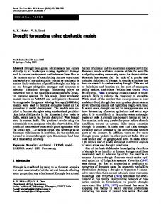
on images have anything like the look and feel of the real world { the best one can do is make them look like clouds (see gure 1).

The outline of this paper is as follows. In x2, we will introduce the precise mathematical formulation of the problem. In x3, we describe the most striking empirical phenomenon exhibited by the statistics of natural images: their apparent scale-invariance. In x4 we digress to show the problems that scale-invariance creates: there are no scale-invariant probability measures supported on image functions. To construct such probability measures, we need their samples to be generalized functions (`distributions' in the sense of Schwartz). In x5, we introduce the basic idea of this paper which is to assume images can be described by a numerical quantity called clutter and that an image with clutter c1 + c2 can be constructed by adding independent images of clutter c1 and c2 . Such a situation is called an in nitely divisible family and we propose that this de nes a natural class of image models. Although not exactly satis ed by the `true' probability measure on natural images, the in nite divisibility assumption captures in simple mathematical terms certain essential aspects of this measure. In x6 and x7 we analyze in nitely divisible image models, introducing two further axioms which express a) the idea that objects are local while the image itself is an ergodic eld and b) that some parts of scale-space are empty of objects, an assumption we refer to as the `blue-sky' hypothesis. After that, we need to convince ourselves that these axioms can be satisi ed. It is not at all obvious that there is any probability model satisfying these axioms (which are closely related to what physicists would call a 2D non-Gaussian conformal eld theory). We do this by establishing in x8 the convergence of what we call random wavelet expansions. In x9 we review recent experiments with images which support the theory we have described. In x10, however, we describe a basic failure of this class of models: the presence of clouds of tiny objects gives the marginal distribution on lter statistics a smooth density. All experiments, however, have resulted in empirical histograms for such statistics which appear singular at 0. We would like to thank many people for help with this paper, particularly: 3

Persi Diaconis for introducing the rst author to the idea of in nitely divisible distributions; Stuart Geman and Zhiyi Chi for very stimulating conversations on scale-invariance and further ideas on the use of in nitely divisible models; Yves Meyer for help on the convergence of random wavelet expansions; SongChun Zhu for many provocative ideas on the modeling of images; and Jinggang Huang for his skill and insight in analyzing the statistics of natural databases.

2 The basic setup We begin by making precise what we mean by an image. Physically, images arise in a camera or in your eyes. Let (x; y; z) be coordinates in 3 space. Assume the world is viewed from the origin (through a `pin-hole' or lens centered at the origin). Then the 2D manifold of viewed directions is the sphere of rays through the origin, or an open set in this sphere (such as the retina). One can put coordinates (u; v) in this manifold, locally near the ray x = y = 0; z > 0 either by spherical coordinates (x; y; z) = (r sin(u) cos(v); r sin(v); r cos(u) cos(v)) for instance, or projective coordinates (x; y; z) = (ru; rv; r). In either case, a nite set of N sensors is positioned suitably to sample the light energy present around particular rays (u ; v)1RRN . The signal received by sensor  may be modeled as the convolution I() = u;v K(u ; u ; v ; v )I(u; v)dudv, where K is the impulse response of the sensor to dierent directions and I is the energy of the incident light. In this very concrete physical situation, the question addressed in this paper is to construct suitable probability measures on the nite-dimensional vector space IRN containing the measurements fI()g. In order to come up with a more mathematically tractable setup, however, we want to simplify the geometry in several ways. First of all, we want to avoid modeling the details of the sensor positioning, modeling the energy I directly. In this case, the simplest mathematical scheme is to consider I as a random distribution and speci c sensors  as de ning test functions K(u ; u; v ; v ), so that I() is the inner product of the distribution I with the test sensor . We therefore seek probability measures (I) on the space D0 of distributions. Moreover, we want to avoid modeling the details of peripheral vision and the borders of images. The simplest way to do this is to construct probability measures on the space of distributions I(u; v) de ned for all (u; v) 2 IR2 . We shall assume the measures we construct are stationary, so that their marginals on the distributions in a speci c window, i.e. in an open subset U  IR2 , are independent of translation. The assumption is that physical images I(u; v) for u; v suciently small are modeled by the marginals of this probability measure. In this case, it does not matter whether we use spherical or projective coordinates 4

in the manifold of rays, because to rst order, in a Taylor expansion: (r sin(u) cos(v); r sin(v); r cos(u) cos(v))  (ru; rv; r): To avoid confusion, note that the measures we seek on I(u; v) do not model random projective views I(u; v) of the world. This is because projective views distort spheres in (x; y; z)-space near the periphery of sight into elongated ellipses in the (u; v) plane. Nor can they possibly model spherical images I(u; v) of the world because spherical images are only de ned for a compact set of values of (u; v). Instead, we are asking for a stationary measure whose windows model actual images of the world locally. The samples from such a stationary measure are more like Chinese landscape scrolls, in which more and more of the world comes into view as the scroll is further unrolled. In passing from a model of a bounded part of the world to the idea of images as in nite scrolls, it is natural to assume that distant parts of the image I are more and more independent. In other words, we make it part of our basic assumption that the measure we construct will be ergodic in a suitable sense. For some theorems it will be important to formulate this requirement quantitatively, for instance by asking that some covariances decay fast enough. But the independence of 2 random variables is much stronger than having zero covariance and one may also want to assume the decay of various higher order measures of dependence such as mutual information.

3 Axiom I: scale-invariance Vision is quite distinct from hearing and touch in its lack of characteristic scale. In hearing, there are many natural units for measuring time: your heart beat, the frequency of your vocal cords, the length of a day, etc. These units give universal scales in which to measure any time interval, hence units in which to record the signal received from your ears. Similarly, when you touch an object, its true physical size determines how many tactile sensors in your skin are excited, hence it always evokes a signal in the 2D array of tactile sensors of the same `size'. But this is not true of vision: you can see your spouse's face from a 100 foot distance or a 1 inch distance and the resulting signals transmitted by your retina are (approximately) scaled versions of each other. What this means is that any scene which produces an image I(u; v) on your retina or camera focal plane may also be viewed from nearer or farther away, producing (approximately) an image I(u; v) which is a scaled version of I. Why have we written `approximately'? The reason is that this ignores perspective eects. In fact, when you get closer to a scene, the nearer objects get larger faster than the farther objects. These eects are not usually very 5

noticeable. Except for unusual views, such as telephoto images down twenty blocks of a straight street or closeup views of a face 1 inch from the nose, the eect is not obvious. The simpli cation we are proposing to use goes under the name of `weak perspective' in the computer vision literature. The characteristic distance to each part of the viewed scene is xed at some typical value z0 and surface points with coordinates (x; y; z) are projected to the image plane via (u; v) = (x=z0; y=z0 ). Then getting closer or moving farther away from the scene simply changes z0 and precisely rescales the image. Whether this approximation is reasonable depends on the stochastic nature of the world geometry, i.e. what is the natural distribution of objects and their sizes in the world which we live in. We will present below some reasons for believing this weak perspective model is reasonable. Mathematically, we may express scale-invariance in terms of the basic probability measure  on D0 as follows. Firstly, the group of dieomeorphisms of IR2 acts on D and on D0 , in two natural ways. Let  : IR2 ! IR2 be a dieomorphism of IR2 . We may de ne T (f)(x) = f(;1 (x)) for f 2 D and de ne it on D0 by transpose-inverse: < T (I); f >=< I; T;1 (f) > , for I 2 D0 ; f 2 D. Explicitly, this makes  act on distributions I which are functions by the rule T (I)(x) = jDj;1I(;1 (x)). Alternately, we can make it operate this last way on D and by the rst formula on D0 . We want to express the invariance of the probability measure  on D0 by the formula

Axiom I (scale-invariance): (T (S)) = (S) for all measurable subsets S  D0 and all  of the form (~x) = ~x + ~a. But which is right de nition of the action? In terms of measures on D0 , the probability of seeing a speci c pattern may be described as (fI j j < I; fk > ;ak j < g), where fk are a set of test functions, e.g. the sensors of a camera, ak are the expected values for these responses and  allows for noise. The probability of seeing the same pattern at a smaller scale is (fI j j < I; gk > ;ak j < g) where nothing changes but the sensors. We need gk (~x) = 2 fk (~x + ~a) where  is the factor by which the pattern shrinks and ~a is a translation. Note factor 2 is used so that the sensor has the RR that the RR same sensitivity, i.e fk dxdy = gk dxdy. These two measurable subsets of D0 dier by the action of the dieomorphism (~x) = ;1 (~x ; ~a), but note that the action is de ned in the second way, i.e. it acts on test functions with the Jacobian factor and on images by simple substitution. Unfortunately, as is well-known, there are no non-trivial measures on D0 which are invariant under translations and scale-changes, which have nite mean and variance. For any such measure , the mean I0 (~x) and the covariance C(~x; ~y) 6

are distributions de ned by: < I0 ; f > = Exp(< I; f >) < C; f g > = Exp(< (I ; I0 ) (I ; I0 ); f g >) (where `Exp' means expectation). Because of translation invariance, I0 is a constant and C is a distribution in ~x ; ~y only. Because of scale-invariance of , C is also invariant under scale changes and hence must be a constant too. Hence the measure  is supported on the one-dimensional subspace of constant images IR
1  D0 . If these moments do not exist, there are translation and scale-invariant measures. The simplest of these is `Cauchy noise'. On a nite grid, this is de ned by independent pixels, identically distributed with a Cauchy distribution. The measure cauchynoise is de ned simply by its Fourier transform: R Exp(ei ) = e; jf (x)jdx :

This problem stems from `infra-red' blow up, i.e. scale invariance of the kind we are assuming implies too many extremely large-scale oscillations and these give rise to in nite energy around zero frequency. The solution is to consider images as distributions modulo constants. Since the large scale, low frequency contributions to the image are locally nearly constants, they have less and less impact on the image modulo constants. This leads us to look instead for measures on the quotient space: Dd0 =def D0 =IR
1 For such a measure, the covariance is a distribution C(~x ; ~y) which is scale invariant modulo constants. If it is rotationally symmetric too, the only such distributions are C(~x ; ~y ) = c1 log(k ~x ; ~y k) + c2. Since the covariance is now only de ned on test functions with mean 0, we can ignore c2 . Measures on Dd0 which are stationary, rotationally symmetric and scale-invariant do exist. The classical one is the Gaussian measure, known as the `two-dimensional free quantum eld': the unique Gaussian measure with mean 0 and covariance ; log(k ~x ; ~y k). It is constructed by approximating Dd0 by nite dimensional R quotients given by nite sets fig; 1  i  n of test functions with i = 0. For each such set, we use the gaussian on IRn with mean 0 and covariance Ci;j =

ZZ

i (~x)j (~y) log(k ~x ; ~y k)d~xd~y:

By standard arguments (see [G-V], Ch.4), these de ne a Gaussian measure on the nuclear space Dd0 . In fact, this measure is supported on a suitable HilbertSobolev space de ned by a negative degree of dierentiability. We may de ne these spaces by: ;s = (I ; 4)s=2 L2 : Hloc loc 7

Then a careful study using the Minlos-Bochner theorem (see [Hi], [Re] as well as [G-V]) shows that it is supported just outside the space of locally L2 functions1 ;. { in fact in \>0Hloc Loosely speaking, this measure is given by the probability density function: RR Y d(I) = e; krI k2 dxdy dI(x; y): x;y

This formula is most easily interpreted by rewriting it in terms of the Fourier transform I^ ofZ ZI. Since ZZ k rI(x; y) k2 dxdy = ( 2 + 2 )jI^(; )j2dd; d can be rewritten, still loosely, in diagonalized form: Y d(I) = e;(2 +2 )jI^(;)j2 dd: ;

This shows that samples from this model are simply `colored' noise, white noise with higher frequencies decreased by the factor k (; ) k and low frequencies ampli ed by the inverse of this factor. The eect is that, unlike white noise, when it is smoothed, the law of large numbers doesn't erase all features, but it always retains oscillations of the same contrast. An example of an image sampled from this distribution is shown in gure 1. We will construct non-Gaussian rotation and scale-invariant measures below. At this point note that, even when non-Gaussian, their covariance must be c1 log(k ~x ; ~y k), hence their power spectrum takes the form: Exp(I^(~1 )I^(~2 )) = ~1 ;~2 ~1 2 k 1 k

4 Non-existence of scale-invariant measures on functions The scale-invariant Gaussian probability measure is well-known not to be supported on the subspace of measurable functions L1loc  D0 ([Do], [Re]). This

1 This holds in any dimension. For any , there is a unique Gaussian probability measure on Dd0 with mean 0 and covariance ( ) = 1 log(k k) + 2 . To see where it \lives", we may construct it from \white noise" (see [Hi]) which is given by ( ) = 0 if 6= 0 or equivalently by: R ExpI ( i ) = ; jf (~x)j2 d~x ;d=2; The scale-invariant measure It is well-known that white noise is supported in \>0 loc is constructed by operating on white noise by convolution with the kernel k k;d=2 which boosts the dierentiability by 2. d

C ~ x

c

x ~

c

C ~ x

e

e

x ~

:

H

:

~ x

d=

8

Figure 1: A computer simulation of a sample of the scale-invariant Gaussian measure on images. makes such a model seem complicated and inaccessible. Mallat, Meyer, Donoho, Simoncelli, Coifman and others have instead proposed various spaces of true functions as natural models for images (see [Ma]). For example, they propose the space of functions I(x; y) of nite total variation, or the more subtle Besov spaces or speci c spaces of wavelet expansions with mother wavelet(s) adapted to image geometry. The point of this section is to prove that there is no scaleinvariant probability measure on such spaces (or on them modulo constants). The idea is that scale-invariance automatically implies oscillations everywhere of the same amplitude and measurable functions cannot be so complex. Thus accepting the stochastic approach to images and their scale invariance forces you to model images by Schwartz distributions which are not measurable functions. It seems that the models of images proposed by the wavelet community are really models of the `cartoon' component J obtained by decomposing an image I into a sum J + n, where n is noise or texture or clutter and J are the major salient parts of the image. But, whereas n has been modeled as noise, we 9

propose that it really follows the same statistics as J only scaled down (compare Meyer's discussion [Me]).

Theorem: Assume  is a probability measure on Dd0 , distributions on Rn mod-

ulo constants. Assume  is invariant by translations and scale transformations and that  is not a delta function with support 0. Then  is not supported on the subspace of locally integrable functions

(L1loc =R
1)  Dd0 :

Proof: Assume  is supported on L =R
1. Fix any positive numbers a and r and let Br (~x) denote the ball of radius r with center ~x. Let jS j denote the Lebesgue measure of a subset S  Rn. For any I 2 L and ~x 2 Rn, de ne ga;r (I; ~x) = jf~y 2 Br (~x)jjI(~x) ; I(~y)j > ag=jBr (~x)j: 1 loc

1 loc

This de nes a measurable function: ga;r : (L1loc =R
1)  Rn ! [0; 1]: In particular, we can integrate ga;r times the measure  and get ExpI (ga;r ) = g a;r (~x). Because  is invariant with respect to translations, g a;r is constant as a function of ~x. Because  is also scale-invariant, ga;r is independent of r too! Thus ExpI (ga;r (
;~x)) = pa for some constant pa depending only on a. Next, consider ga;r (I;~x) for xed I and r ! 0. Recall that Lusin's theorem for the function I states that I is \almost everywhere continuous." More precisely, for every 2> 0, there is a set Z2  Rn with jZ2 j 2 such that I j( n;Z2) is continuous. Recall that if S  Rn is measurable, S has density 1 at a point ~x 2 S if: lim jS \ Br (~x)j=jBr (~x)j = 1 r!0 and that there is always a set Sbad  S with jSbad j = 0 such that ~x 2 S ; Sbad implies S has density 1 at ~x. Combining these two shows that

R

lim g (I;~x) = 0 r!0 a;r But

if ~x 2 (Rn ; Z2 ) ; (Rn ; Z2 )bad : \

Z0(I) = [Z2 [ (Rn ; Z2 )bad ] 2

has measure 0, hence for xed I and ~x 62 Z0 (I) lim g (I; ~x) = 0: r!0 a;r 10

[

Note that Z0 = Z0 (I) is a set of measure zero in (L1loc =R
1)  Rn. I

Now apply Lebesgue's bounded convergence theorem: pa = rlim !0 ExpI (ga;r (I;~x)) = ExpI (lim g (I;~x)) r!0 a;r = 0: Thus for every a and r, ga;r = 0 for almost all I and ~x. This can only happen if the set of non-constant I has -measure 0, i.e.  is a delta function supported on 0. This proves the theorem.

5 Axiom II: clutter and in nite divisibility A fundamental fact about the world (or, at least, about the way we think about the world) is that it is not a formless mixture of stu, but is broken up into discrete objects. Individual objects are the things which we name, the things we pick up and the things which have a speci c use. What constitutes an object is never precise: objects typically are made up of parts, which may be thought of as distinct objects, and are part of larger assemblages which can be treated as single objects. The prototypical object is a simple rigid thing made of a single material with a homogeneous appearance which can be moved independently of the rest of the world, e.g. a knife or a stone. But most objects are more complex and have parts: a body is a single object (e.g. it resists dismemberment), but it is made of parts { limbs, trunk, head, etc. { which move as separate almost rigid objects. Other `objects', referred to in language by so-called mass nouns, break up into tiny parts. Thus sand is made up of a huge number of grains. Since the 3D world breaks up into objects, the 2D views produced by imaging the world also break up into the viewed surfaces of each object. Visually, simple objects are most readily identi ed by their motion relative to the rest of the image, e.g. by their simple optic ow elds; but they often appear clearly in static images by virtue of their homogeneous color or texture, separated from the background by sharp intensity or local power spectrum discontinuities. It is natural to break up 2D views of single objects into further parts on the basis of albedo changes as well as its 3D parts. For instance, if the surface of a sweater is variously colored, its pattern breaks its visible surface into distinct 2D surface parts. In other cases there is a mixture of geometric and illumination factors that break a surface into parts. For instance, the visible surface of a lake may break up into vast numbers of ripples. You may also treat shadows and 11

highlights as `parts' of the surface, objects in the 2D world of the image. From the point of view of images, all these eects break up a part U of the image domain into subparts Ui  U which we will consider as being the viewed portion of a virtual object, an in nitely attened object on the surface of another. Can we express the fact that images depict a world of objects as a mathematical property of the probability measure  on images? This property is not a simple one to capture, but, as a rst approximation, we propose that it means that the measure  is in nitely divisible. Recall that a probability measure  on R is in nitely divisible if, for every n  2, there is a probability measure n such that  = (n)  (n) 


 (n) (where  represents convolution). Translating this into the language of random variables, if x is a random variable distributed by , then for every n, x can be written as a sum x = x1 + x2 +


+ xn, where xi are `iid', independent and identically distributed. It is a theorem that in nitely divisible distributions belong to semi-groups of distributions (see e.g. [Sa]), i.e. for each such , there is a a family of measures t , de ned for all t  0, such that  = 1 and s  t = s+t . The measures (n) in the de nition are just the measures 1=n in the semi-group. This gives us the intuitive characterization of in nitely divsible distributions as the marginal distributions on the value X1 of stationary stochastic processes fXt; t  0; X0 = 0g with independent increments: i.e. the distribution of Xt1 ; Xt2 depends only on t1 ; t2 { it will be t1 ;t2 { and it is independent of Xs1 ; Xs2 if the intervals [t1; t2] and [s1; s2 ] are disjoint. The same de nition works for vector-valued random variables as well as scalar random variables. Thus we de ne a probability measure  on a function space E to be in nitely divisible if for every n  2, there is a probability measure (n) such that  = (n)  (n) 


 (n) . Then there is a semi-group t as before and a random variable in E chosen from  is an iid sum of n random variables in E chosen from (n) . Thus, for images I, we propose:

Axiom II (in nite divisibility): 1. Every image I has associated with it a parameter c, the clutter of I, 2. Images with clutter c are random samples from a probability measure c on D0 and c  d = c+d . This is equivalent to saying that an image I with clutter c can be formed as a sum I = I1 + I2 +


+ In , where Ik are independent images each with clutter c=n. What we have in mind is to create an image with a certain level of clutter 12

as the superposition of images with less clutter. This is clearly a toy version of the way nature makes the real world, starting with bare land, adding rocks, trees, animals more or less at random. It is not meant to be exactly true of the distribution of generic images, but we propose it as being approximately true, like the axiom of scale invariance. Let us try to be clearer about `how true' this axiom is for real world images. It seems reasonable to imagine the world as being formed by placing objects in a scene, some simple, some compound, some in large arrays and by painting their surfaces with patterns and shadows made up of other shapes, simple, compound and textured. This scene is then viewed from a random viewpoint. If we make simpler scenes by leaving out all but a few of its component objects and surface shapes, we can imagine recreating the full scene by adding together these simpler scenes. This will work except for one main phenomena which won't be captured. This is partial occlusion. Imagine a scene with two objects O1 ; O2 viewed from some point P . If neither occludes the other, the resulting image is the sum of the images of the two separate objects. If O1 is in front of O2 and its outline is wholly inside of O2's, then the resulting image is the sum of O2 and that of O1 but painted with the dierence of the colors of O1 and O2 . The hard case is when one object partially occludes the other: this results in `T-junctions' where their contours intersect and the object in front must be painted so as to cancel out the occluded portion of the contour of the object in back. This cannot be done without violating independence of the two simpler images. Thus we propose that T-junctions in images are the simplest structures which violate the in nitely divisible axiom. In addition to T-junctions, partial occlusion produces extended contours which are broken into pieces, which also cannot arise from an in nitely divisible distribution.

6 Axiom III: Locality of objects and ergodicity The above two axioms are nearly all we want. In fact, a remarkable fact is that in nite divisibility nearly produces objects for us. To see this, we need the famous Levy-Khintchine theorem which makes very explicit the nature of in nitely divisible distributions. Looking rst at the case of scalar random variables x with distributions , the Levy-Khintchine theorem, in its usual form, asserts the existence of an auxiliary measure , called the Levy measure, on IR ; (0) such that x2([;1; 1]) < 1 and: Z

eix (dx) = eix0 ;2 2 =2+^ () ;

where ^ is the Fourier transform of , interpreted by de ning the principal part of  as a distribution. 13

This theorem can be rewritten as an explicit recipe for constructing the random variable x: x = x0 + x1 + i2xi ; where x0 = a constant x1 = a standard normal variable x2 ; x3;


= a Poisson process on IR ; (0) with density  The theorem should be understood to mean that the random variable x has a xed part, a Gaussian part and a discrete part which is the sum of a Poisson process, i.e. a countable set of points in IR ; (0) distributed randomly with density given by the measure . The simple case is where (IR ; (0)) < 1, so that the Poisson process consists in a nite set of points and the sum in the discrete part is nite. In this case the Fourier transform ^ of the measure  exists in the usual sense. To include all in nitely divisible distributions, however,  must be allowed to have in nite measure around 0 so long as x2 assigns nite measure to a neighborhood of 0. In this case, we have to add convergence factors to the series for the discrete part of x (and the series must be summed in the right order). We ignore these technicalities. The important case for us are those scalar random variables x such that x = x0 + i xi ; fxi g Poisson for a nite measure : We may think of these variables as scalar variables resulting from the superposition of a nite number of `objects'. It is a standard result that such x's are exactly those with in nitely divisible distributions and Pr(x = x0) > 0 (i.e. their distributions have `atoms'). The Levy-Khintchine theorem generalizes to random variables I with values in Banach spaces X (see [Li]): I = I0 + I1 + i2 Ii ; where I0 = a constant I1 = a Gaussian random variable I2 ; I3;


= a Poisson process on X ; (0) with density  As before, the Levy measure  is a measure on X ; (0) with possible singularities at 0, and the sum has to be interpreted carefully if this singularity is too big. We want to apply this to the probability measure on images, with X  Dd0 being a Banach subspace of the full space of distributions (modulo constants) which carries the measure . The meaning of the samples Ik ; k  2 from the Levy measure is that these component images are the primitive `objects' out of which 14

images are composed. Thus we add our third locality axiom which states that these objects are given by functions and are compactly supported:

Axiom III (locality): The Levy measure  for images I is sup-

ported on the space L1c of measurable functions with compact support.

(Note that L1c is a subspace of D0 d because, among all the functions f +a; a 2 IR, only one can have compact support.) What happens when we combine axioms 1, 2 and 3? From in nite divisibility we get the Levy-Khintchine decomposition of I. From scale-invariance and the uniqueness of the Levy measure, we conclude that  must also be translation and scale invariant. In other words,  is invariant under the three-dimensional group G = IR2 IR+ of maps (x; y) ! (rx+a; ry+b). By axiom 3,  is supported on L1c . Denote by p : G  L1c ! L1c the action of the group G on our function space. On the other hand, there is a measurable map L1c ; (0) ! IR2  IR+ taking every non-zero function f to the center and radius of the unique smallest circle on which it is supported. Let L1u  L1c be the set of functions whose support is contained in the unit circle and in no smaller cirle. Note that acting by (a; b; r) 2 G carries the unit circle to the circle with center (a; b) and radius r. So combining these two maps, we get a measurable isomorphism: IR2  IR+  (L1u ; (0))  = L1c ; (0) de ned from the LHS to the RHS by the action of the group and from the RHS to the rst two factors on the left by the smallest circle construction. The scale invariance of the Levy measure then means that, in this product decomposition, it is a product of Haar measure dx:dy:dr=r2 on the group and a reduced Levy measure u on L1u :  = dx:dy:dr r  u:

7 Axiom IV: Blue sky We next want to consider the reduced Levy measure u. A fundamental property of the world and of images of it is that they have blank spaces in them: the blue 2 Confusingly, 3 is the left is the right invariant Haar measure and invariant Haar measure. If the group acts on functions in the usual way, we believe the right-invariant measure on the group makes the product measure invariant. da:db:dr=r

da:db:dr=r

15

sky, blank painted walls. This is really a property of scale-space. When things on all scales and at dierent locations are put together in a scene, there should be parts of scale-space which are not sampled. This eect can arise from the natural uctuations of the sampling density of the Poisson process, but only if the Levy measure is not too big. In order that our model will produce images with blank regions in them, we assume:

Axiom IV (blue sky) 1. The constant image I0 is zero, 2. The Gaussian component I1 is zero and 3. The reduced Levy measure u is nite. This axiom implies that the Poisson process Ii sampled from  can be constructed from a Poisson process (ai ; bi; i ) in the group G with density cdadbd= plus independent random choices Ji sampled from u. Thus it gives us the explicit form of the expansion: I(x; y) = i Ji (i x + ai; i y + bi ): We want to call such an expression a random wavelet expansion. The terms in this expansion are meant to model the individual `objects' in the scene (where objects is interpreted to include things such as parts of patterns, shadows, textons, etc, as discussed above). The above axiom implies that for any bounded part K of G there is a non-zero probability that the series for I contains no term with (ai ; bi; i) 2 K. This means that the resulting image I contains no objects of a certain bounded range of sizes in a certain bounded part of the image plane, hence images have nearly blank areas, when blurred to eliminate in nitesimal features and considered mod constants to eliminate huge features. It is not clear, however, that any measure of the above type exists. The series clearly converges if we put infra-red and ultra-violet cutos, but this is not clear in the full scale-invariant case. The convergence for this case is discussed in the next section. What do such random wavelet images look like? We have simulated them for several choices of u and displayed the results in gures 2-3. In the rst image, u is supported on the characteristic functions of circles and the clutter is low to show the individual terms of the expansion clearly. Each is colored by a Cauchy random variable and the whole image is displayed with a gamma correction, applying a sigmoidal function 1=(1 + exp(;I=c). (This is supposed to mimic 16

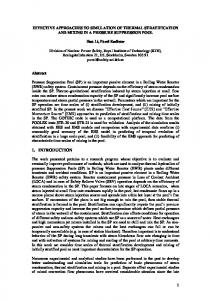
real images where the typical ratios of maximumto minimumintensities are 1001000 and are displayed by lm with some gamma correction to compress the dynamic range.) In the next two images, circles are replaced by `ribbons' (also called `worms' or `snakes') obtained by sweeping a circle of varying radius along a curve called its medial axis. In the simulation, the orientation of the medial axis and the log of the radius are given by independent Brownian functions of arc length and the length of the axis is exponentially distributed. In the last image, the support of every function in u is a rectangle but it is not colored with constant intensity but by a sum of a constant and of three random sine-waves.

8 Convergence of Random Wavelet Expansions In this section, we want to prove that, with mild conditions on the functions in the support of the Levy measure , the random wavelet expansions (7.1) converge almost surely as distributions. We saw in x4 that they cannot converge almost surely as functions because they would then de ne a scale-invariant probability measure on functions. However, it turns out that, like samples from the scale-invariant Gaussian model, random wavelet expansions live \just outside" functions. Let us x our notations. It is no extra work to consider \images" on Rd for any dimension d. De ne as usual:

D D0 Dd Dd0

= = = = s H = kf k2s =

D(Rd) = C 1 functions with compact support 0 (Rd) = dual of D; generalized functions D Z   f 2 D d f(x)dx = 0 R dual of Dd = D0 =R
1 Hilbert-Sobolev space with norm Z 2 s=2 ^ ~ 2 ~ (1 + k k ) jf( )j d

Z

((1 ;
)s=2f
f)d~x Ks (~x) = ((1 + k~k2);s=2) b (~x); the semigroup of \Bessel" kernels, s  0 = cnst:k~xk s;2 d K d;2 s (k~xk); where K is the classical Bessel function: =

Thus

Ks  H t = H t+s ; all t; s  0:

17

20 40 60 80 100 120 140 160 180 200 50

100

150

200

20

40

60

80

100

120

140

160

180

200 20

40

60

80

100

120

140

160

180

200

Figure 2: A computer simulated sample of random wavelet images, one with low clutter and disk-like primitives, one with higher clutter and textured rectangular primitives. See text for details.

18

20 40 60 80 100 120 140 160 180 200 50

100

150

200

50

100

150

200

20 40 60 80 100 120 140 160 180 200

Figure 3: Computer simulated samples of two random wavelet image with ribbon-like primitives. See text for details. Finally de ne H

0 loc

= functions with

Z

K

f 2 < 1; all bounded K:

;s = (I ; 4)s=2 (H 0 ); s  0: Hloc loc 19

As above, let u be the reduced Levy measure supported on functions whose support is contained in the unit ball (and no smaller ball). We want to assume u is supported in a fractional Sobolev space. The reason this is useful is that natural models for the elementary components of images may include functions which are smooth on a domain K with smooth boundary, but 0 outside K thus discontinuous on @K. Such functions are typically in H s for all s < 1=2. We shall prove:

Theorem: Assume that for some  > 0 Z

kJ k2 du(J) < 1:

Then the random wavelet series:

I(~x) =

X

Ji (i x~0 ; x~i ); ~x 2 Rd

i

s =R
1, all s > 0. converges almost surely in Hloc

Proof: We shall show that for all s > 0, the series Ks  I converges almost surely in H =R
1. Break up the formal series for I as follows: 0 loc

I(~x) = Ik (~x) =

X

Ik (~x) k2ZZX 2k i 16 or not. The result is a simpli ed 3  3 block of small numbers, which most often is either all 0's (background blocks with intensity variation less than 16: about 65%) or all 0's and 1's (blocks showing edges or corners with roughly two grey levels present: about 20%). They look at the following two statistics: a) z de ned by the range [0; z] of the simpli ed block and b) conditional on z = 1 and the block being divided into a connected set of 0's and a connected set of 1's, the number y of pixels in the component not containing the center pixel. They calculate the distributions of z and y for their database of 80 images and for downscaled (2  2 block averaged) images. The two histograms appear identical to within experimental uctuations. 25

2 0 −2 −4 −6 −8 −10 −12 −14 −16 −18 −20 −1

−0.8

−0.6

−0.4

−0.2

0

0.2

0.4

0.6

0.8

1

Figure 4: Histograms of wavelet coecients on four dierent scales. The vertical axis is log probability and the four curves have been shifted vertically to separate them. The wavelet scheme used is Simoncelli and Freeman's steerable pyramid [S-F] and the images are from the database of van Hateren [vH].

9.2 In nite divisibility We have performed some experiments to see whether the in nite divisibility axiom holds approximately for real data. In one experiment, 18 scenes were acquired around a house, garden and the nearby streets using an Apple QuickTake camera. The camera's response was calibrated using an optical gray card. These images were rst tested for scale-invariance. The full images were 480 by 640 and seem to be smoothed by the hardware set-up, hence all measurements were done on block averaged 2  2, 4  4 and 8  8 blow-downs. If the images had scale-invariant statistics, the gradients of these 3 images would have identical histograms. To measure the departure from scale-invariance, we t the log of the variances of the gradients as above. Expressed in terms of power spectrum fall-o, we found scaling exponents C=  with 's in the range [1:94; 2:12] for the 14 out of the 18 images showing vegetation and in the range [2:18; 2:3] for 4 images of interior scenes without complex textured objects. According to the in nite divisibility axiom, we should interpret this as meaning 26

that the 4 interior scenes are samples from the prior with less clutter, while the other 14 are samples from more cluttered priors in the same in nitely divisible family. The four interior scenes can be identi ed by 3 properties: the variances of the image gradient were smallest; the histograms of the image gradient were most sharply peaked; and they all represented clean clutter-free interior scenes. A second subset of 4 images was chosen from the remainder by the opposite properties: the variances of the image gradients were the largest; their histograms were broadest; and they all represented cluttered garden scenes. We then formed the composite histogram of nearest neighbor pixel dierences for each set. If we have sampled two points in a semi-group of in nitely divisible distributions, we should be able to reconstruct approximately one histogram from the other by the following procedure. Taking one histogram h1, form its Fourier transform, raise it to a suitable positive real power and take the inverse Fourier transform. If the power is greater than one, this operation smooths the histogram hence is stable; but when it is less than one, it is unstable. So for powers less than one, we introduce a high frequency cuto, by multiplying the Fourier transform by a Gaussian (or, equivalently, convolving the original histogram with a Gaussian). The results are shown in gure 5. The best tting powers turned out to be 3.8 and 1/3.8, i.e. the garden scenes were 3.8 times as cluttered as the interior scenes. Although this is a rather weak test for in nite divisibility, it does lend some credence to our Axiom II.

9.3 Blue Sky We have no experimental tests for the locality axiom! It is hard to imagine how you could have a sensible model of the real world with in nite divisibility and without locality. The samples from the Levy measure are meant to represent elementary objects or parts of objects and these should be local. However, the blue sky axiom has one very strong piece of evidence supporting it: this is the presence of sharp peaks in the probability distribution of lter responses at 0. In every case we have examined, for every database and every lter with mean 0, this peak seems to be present. In the cases where the clutter is less and the lter is matched to typical image features (like edges), the peak is much more pronounced. If the clutter is greater or the lter has no geometric signi cance (e.g. a random set of +1's and -1's of equal number), the peak is less pronounced. This has a clear interpretation for in nitely divisible distributions. Note that if  =  0 +  00, then the corresponding distributions satisfy p = p0  p00. The basic idea is that the bigger the Levy measure, the smoother the distribution. Thus i) p is C 1 whenever the Levy measure has a Gaussian component, and on 27

−7

−8

log of probability

−9

−10

−11

−12

−13 −1.5

−1

−0.5 0 0.5 log(I )−log(I ), I and I adjacent pixels

1

1.5

−0.5 0 0.5 log(I )−log(I ), I and I adjacent pixels

1

1.5

0

1

0

1

−5

−6

−7

log of probability

−8

−9

−10

−11

−12

−13

−14 −1.5

−1

0

1

0

1

Figure 5: Top: Adjacent pixel statistics for the 4 garden scenes (represented by dots) versus the 3.8-th convolutional power of the adjacent pixel statistics for the 4 interior scenes (represented by the solid line). Below: Adjacent pixel statistics for the 4 interior scenes (represented by stars) versus the 3.8-th convolutional root of the adjacent pixel statistics for the 4 garden scenes (represented by the solid line). the other extreme ii) p has a delta function component if and only if the Levy measure is nite. A simple example to keep in mind is the in nitely divisible gamma family of distributions. Here  = x1 e;x dx; x  0 and pt = ctxt;1e;x for suitable constants ct . Note that pt is in nite at 0 if t < 1 and gets more 28

and more dierentiable at 0 as t ! 1, but never becomes C 1 . A symmetric version of this is given by the family with even Levy measure  = jx1j e;jxj dx and pt = ct jxjt;0:5Kt;0:5(jxj), where Kt are the mod ed Bessel functions. Then p1 = 0:5
e;jxj and pt(0) = 1 if t  0:5. These two examples are included in the general theory of self-decomposable distributions. These can be de ned by requiring  = jxjf(x)dx where f, restricted to the positive axis is decreasing, and restricted to the negative axis is increasing. In this case, the pt are all unimodal with maxima at 0 and pt (0) = 1 if and only if f(0) < t.

10 A problem: Small objects and the smoothness of lter marginals The main result of this section is that, when images are formed by a scaleinvariant process, there will be clouds of tinier and tinier objects everywhere and a kind of central limit theorem will take over. The eect turns out to be that images will be the sum of a Cauchy-like component and a second component independent of this; and the Cauchy-like piece will have a smooth (C 1 ) distribution, hence so will the sum. Here's how we make this precise: rst assume that the reduced Levy measure u is not supported entirely on functions with mean 0. We will return later to remove this restrictive hypothesis. We introduce the following notation: for any test function f 2 Dd , the lter response I(f) is also in nitely divisible and its Levy measure is the image of that of the Levy measure (J) of I under the map J 7! J(f), (excluding any atom at 0). We call this Levy measure f . Then we have the theorem:

Theorem: If the reduced Levy measure is not supported in Ld = ff 2 L j R f = 0g, and if f is any test function which is constant in some small open set U , 1

1

then the Levy measure satis es:

f  jCxj12 dx [0;a] ;

for some positive constant C1 and non-zero a.

Recall from x6 that  = dxdydr r  u hence f is the image of the measure dxdydr  u(J) under the map: r (x; y; r; J) 7!

ZZ

J(ru ; x; rv ; y)f(u; v)dudv 2 IR:

Now choose (u0; v0 ) 2 U and assume that U contains a disk around (u0; v0) of radius r0. Then we are interested in the translated and scaled versions of J whose support lies entirely in this small disk: this holds if r > 2=r0 and 29

k ( xr ; yr ) + (u0; v0) k< r0=2. Let V denote this set of triples (x; y; r). When this holds, f is a constant on the support of the translate of J and we get: ZZ ZZ 0 0 y 0 0 J(ru ; x; rv ; y)f(u; v)duvv = r;2 J(u0; v0 )f( u r+ x ; v + r )du dv ZZ = r;d f(u0 ; v0) J(u0 ; v0 )du0dv0 : Thus





f   dxdydr   (J) ; u r V RR where (x; y; r; J) = r;2f(u0 ; v0) J. Now the area of the allowed circle in the (x; y) plane is (rr0 =2)2, so we have: 





f  0 (r0=2)2 rdr  u(J) ; r2=r0 RR

where 0(r; J) = r;2f(u0 ; v0 ) J. But the image of the measure rdrjr2=r0 under the map x = r;2 is just 2xdx2 0