cognition and machine learning, and introduces the concept of stochastic ... have been represented as probabilities, and finally the logical development.
Chapter 2
STOCHASTIC COMPUTING SYSTEMS B. R. Gaines Department of Electrical Engineering Science University of Essex, Colchester, Essex, U.K.
1. INTRODUCTION The invention of the steam engine in the late eighteenth century made it possible to replace the muscle-power of men and animals by the motive power of machines. The invention of the stored-program digital computer during the second world war made it possible to replace the lower-level mental processes of man, such as arithmetic computation and information storage, by electronic data-processing in machines. We are now coming to the stage where it is reasonable to contemplate replacing some of the higher mental processes of man, such as the ability to recognize patterns and to learn, with similar c!,pabilities in machines. However, we lack the "steam engine" or "digital computer" which will provide the necessary technology for learning and pattern recognition by machines. In the summer of 1965 research teams working on these topics in different parts of the world discovered, quite independently, a new form of computer which might provide the necessary technology. The "stochastic computer" (1-7), as this has come to be called, is unlikely to prove the ultimate answer to the technological problems of machine learning and pattern recognition. It is, however, a step in the direction of processing by parallel structures similar to those of the human brain, and is of great interest in its own right as a novel addition to the family of basic computing techniques, and as a system which utilizes what is generally regarded as a waste product-random noise. This chapter reviews the data-processing requirements of pattern recognition and machine learning, and introduces the concept of stochastic computing through the representation of analog quantities by the probabilities of discrete events. The first part of the chapter gives a complete overview of stochastic computing and its relationship to other computational 37
38
Stochastic Computing Systems
[Chapter 2
techniques. Later sections treat various forms of stochastic computer in some detail, and outline the theoretical basis for computing with probabi~ listic devices. The final sections describe various systems for pattern recognition and control where the use of stochastic computing elements is advantageous.
1.1. Summaries of Contents of Main Sections Section 2 analyzes the computational problems of learning machines and pattern recognizers, and discusses to what extent the conventional general-purpose digital computer solves them. Matrix operations are taken as an example of generally important computations for which a generalpurpose machine is very slow compared with alternative approaches. It is concluded that in machine learning and pattern recognition one is inexorably driven toward a data-processing system which makes maximum use of every single gate for computational purposes, and has parallel rather than sequential processing. Section 3 examines the nature and origins of stochastic computing. The representation of quantities by probabilities is first introduced and constrasted with the representation of numbers in other forms of computer. Examples are given of two previous computing systems where numbers have been represented as probabilities, and finally the logical development of this concept in work on learning machines is outlined. Section 4 is an exhaustive account of three stochastic computing systems which utilize linear mappings from quantities to probabilities. The first representation is for unipolar quantities; the second maps bipolar quantities onto two lines; and the third representation maps bipolar quantities onto a single line. These last two representations give rise to families of computing elements which correspond closely to those of the analog computer. Stochastic computing elements for addition, subtraction, multiplication, squaring, integration, and interfacing are described for each representation. Implicit function generation for division and square~root extraction is outlined and, finally, the generation of discrete random variables using random noise, or pseudorandom feedback shift registers, is analyzed. Section 5 gives an overview of some of the theoretical foundations of stochastic computing which lie in stochastic automata theory, and discusses the relationship between the economy of stochastic computing and equivalences between stochastic and deterministic automata. Section·6 extends the results of Section 4 to include alternative stochastic representations of quantity, particularly those in which infinite quantities have a definite representation.
Sec. 2]
Machine Learning and Pattern Recognition
39
Section 7 gives a detailed analysis of the main sequential element of the stochastic computer, the generalized integrator or ADDlE. The behavior of the ADDlE as a smoothing element is compared with that of an equivalent deterministic process, and the optimality of the linear ADDlE as an estimator is demonstrated. Section 8 gives the first example of a system where stochastic behavior is essential to the operation. Digital adaptive threshold logic in which the weights take a finite set of values is shown not necessarily to converge to a solution, even when one is within the range of the weights. An alternative, nondeterministic, adaptive algorithm is shown to converge whenever a solution exists, and an example is given of a speech and character recognition system which has been constructed using stochastic feedback. Section 9 reviews the modeling of linear systems using steepest-descent techniques, and analyzes the effect of replacing analog multipliers with switching elements, such as relays. An experimental comparison between six identification techniques, including polarity-coincidence correlation and three stochastic techniques, is outlined, and the different approaches are contrasted in their speed of response, interaction between estimates, bias due to noise in the system being identified, and variance of the final estimates. Section 10 gives a further ~f\ample of system identification where the use of stochastic computing elements enables a computation to be carried out in a way which would be otherwise impossible. The technique is one of maximum likelihood prediction based on Bayes inversion of conditional probabilities, and a particular form of ADDlE is described which enables normalized likelihood ratios to be estimated directly, and in a form suitable for prediction. Section 11 considers some functional networks of stochastic computing elements for coordinate transformations, and the solution of partial differential equation, and compares them with networks of artificial neurons.
2. COMPUTATIONAL PROBLEMS OF LEARNING MACHINES AND PATTERN RECOGNIZERS 2.1. Character of Computations Required in Machine Learning and Pattern Recognition (7a.7b) There are so many different approaches to machine learning (8.9) and pattern recognition (10.11) that it might seem impossible to draw any general conclusions about the nature of their computational requirements. However, whatever the algorithms used in the machines, there are certain character-
40
Stochastic Computing Systems
[Chapter 2
istics of their environments, and the problems they are required to solve, which seem to be of general occurrence. The data input to the machines is generally very great and derived from a large number of coexistent sources, and the number of different inputs which the machine may receive is usually several orders of magnitude greater than the number of outputs from the machine: it has to perform a very substantial reduction of a large data stream. For example, an alphanumeric character recognizer with an input retina of 10 X 10 photocells has at least 2100 possible inputs and about 64 possible outputs-a data reduction of order 1028• The human eye has some 108 photoreceptors, roughly corresponding to a 104 X 104 array, and it is not beyond the bounds of present technology to fabricate an electrooptical array with the same capacity. Having generated this massive data source, however, how one reduces the 108 binary inputs to obtain a meaningful classification of the optical input is another matter; it clearly does not solve the problem to send 108 signal wires elsewhere. Secondly, the adaption, or learning, of the machines, although one of their most complex characteristics, may be regarded, in a computational context, as requiring that the data-reduction procedure be variable. Since this variation will be a function of the "experience" of the machine, it implies some feedback from the results of past data-processing to that at present. The machine must have internal parameters controlling the processing of information which can be adjusted as a result of the effects of previous processing. Thirdly, it is also a general characteristic of machine learning and pattern recognition that the data input is, in some sense, redundant, and the machine does not have to make very fine discriminations based on small differences in the incoming signal. This effect is difficult to quantify, but it seems a universal, and very important, characteristic of the situations in which learning machines and pattern recognizers are expected to operate. Insofar as the computation is concerned, this means that the data processing is global, over whole regions, rather than local, and that any particular part of a computation does not have to be performed to high accuracy; a "law of large numbers" operates to give sensible overall results from a large number of rough local computations. Up to this point learning machines and pattern classifiers have been grouped together, but it is worth noting their similarities and differences. They are similar in that both are devices with inputs and outputs, and a variable relationship between input and output contingent upon the results of previous input/output decisions. They differ in that a pattern recognizer's
Sec. 2}
Advantages and Disadvantages of Sequential Computation
41
decisions generally do not affect the sequence of inputs which it is receiving, while the outputs (actions) of a learning machine feed back into its environment and act to change it. Because of this, the decisions of a pattern recognizer may generally be evaluated one by one and its input/output relationship changed accordingly, whereas the decisions of a learning machine may be evaluated only over a period of time. For direct comparison, therefore, a complete sequence of inputs to a learning machine should be thought of as equivalent to a single input to a pattern recognizer. Hence, over eight successive steps a learning machine with a to-bit binary input pattern has to cope with as much data as a pattern recognizer with 108 cells in its retina. Thus the problems of machine learning are similar, but generally more difficult, than those of pattern recognition. Thus the computational problems of machine learning and pattern recognition may be summarized as: the processing of a large amount of data with fairly low accuracy in a variable, experience-dependent way. In the following sections the defects of a conventional, stored-program, general-purpose digital computer for this type of problem are considered, in order to illustrate the necessity for new forms of data-processing hardware in the physical realization of learning machines and pattern recognizers.
2.2. Advantages and Disadvantages of Sequential Computation No one can fail to be aware of the achievements of the general-purpose, stored-program digital computer, which, in the quarter of a century since von Neumann made the first step from the physical patching of ENIAC to the program control of EDV AC, has had an unequalled impact on scientific and commercial data processing. The size and financial performance of the computer industry indicate the degree of practical utilization of the digital computer, and it is clear that there is room for much expansion yet-in particular through multiaccess, interactive systems where the man and machine may become true partners. However, in the very strength of the conventional digital computer, its sequential, stored-program control, lies its greatest weakness insofar as pattern recognition and learning are concerned; this manifests itself as a tradeoff between the size of a computation and the speed of its solution. The essential structure of a conventional digital computer is a comparatively simple arithmetic/control-unit coupled to a large, uniform store structure, generally based on magnetic cores. The arithmetic unit operates on small units of data stored as bit-patterns in one part of the store, and
42
Stochastic Computing Systems
[Chapter 2
the sequence of operations which it performs are determined by a program in another part of the store. Although the operations of the arithmetic unit are, in themselves, very simple, long sequences of these operations may be used to build up more complex transformations on the bit-patterns in the core store. For example, the user may write a MULTIPLY subroutine, which combines SHIFT operations, ADD operations, conditional JUMPS, and store TRANSFERS, into a routine which takes two binary numbers in named store locations and replaces them with their product. He may then use this routine in many places in his program, calling each time on the single copy which constitutes the subroutine. Such a procedure is obviously very flexible, in that the user-defined routines can perform virtually any operation, and it is also very simple and economical in use, since the one routine may be called by a single JUMP-TO-SUBROUTINE instruction. However, the breakdown of basic operations into a sequence of steps and the use of one operator (subroutine) many times in a program have important disadvantages, in that the times taken by each simple step take longer and longer to perform. In the following section matrix multiplication is taken to illustrate this effect, and both the disadvantages of the generalpurpose computer in performing this operation, and the centrality of matrix operations in machine learning and pattern recognition, are demonstrated.
2.3. Computation of Matrix Operations Xj
.
Suppose we wish to multiply an N X N square matrix Aij by a vector The computation has the form that the product Yi is given by N
Yi
= .:E
A;jXj
(1)
j=l
Thus to compute one element of the vector Y i using a general-purpose computer requires N additions and multiplications (together with store transfers and step counting), and to compute all N elements requires N2 additions and multiplications. Now consider how the requirement to perform matrix multiplications might have arisen: in a typical engineering problem the matrix might be the voltage/current transfer equations for a network of resistors, and the multiplication of a vector by the matrix corresponds to the computation of currents in various legs of the network given the voltages at its inputs. Think now of the behavior of the original network when the same voltages are applied to it and the currents measured: it "computes" the output
Sec. 2]
Computation of Matrix Operations
43
currents, not through a sequence of steps, but in one single step; the factor of N2 times some fairly long time interval has dropped to 1 times a very much shorter time interval. This reduction is of very great importance as soon as the matrix becomes large in size; for N = 100 it is a factor of some 100,000 times. The speed advantage of a resistive network in performing matrix "computations" is very substantial. Karplus and Howard (12) have taken advantage of this in a hybrid computing system consisting of a generalpurpose machine coupled through a digital-analog interface to a network of resistors. In use the general~purpose machine sets voltages into about 1000 transfluxor analog stores, and these drive the network of resistors representing the coefficients in the matrix. Analog-to-digital conversion channels enable the digital machine to read off voltages and currents in the network. Karplus (13) has used this system to investigate the dynamics of water flow in the Californian underground basins. The basic equations to be solved are two-dimensional diffusion partial differential equations, but the shapes of the basins, and hence the boundary conditions, are unknown; simulation results must be checked against field experiments and the boundaries adjusted for the best fit. If this computation were performed entirely by the general-purpose machine, 95% of its time would be allocated to the matrix inversion; when this latter operation is performed by the resistive network the time taken is decreased by a factor of at least ten. The operation of matrix multiplication is not at all atypical, and in fact it is a very common one which underlies many algorithms for machine learning and pattern recognition. For example, in the STeLLA (8.14) learn~ ing system the behavior of the machine's environment is modeled by a set of transition probabilities among the possible states in the environment for a given action. Given an expected probability distribution over the set of states, the distribution which will follow an action is obtained by multiplication of the given distribution by the matrix of transition probabilities for the action. The environment of the simplest STeLLA machine, with a 1000 and ten-bit input pattern, has about 1000 possible states, so that N the speed advantage of matrix multiplication through a resistive network over a digital computer is at least some ten million to one. The importance of matrix operations in general "image transformation" has been discussed by PoppeIbaum et al. (Z); they point out that matrix operations on the points of a retina provide general linear transformations including: (1) translations, rotations, and magnifications, (2) conformal mappings, (3) convolutions, and (4) Fourier transforms. The defects of the general-purpose machine in performing these operations led
44
Stochastic Computing Systems
Sec. 2]
[Chapter 2
A~omparison
of Sequential and Parallel Processing
The analog computing system based on a network of resistors is faster in performing matrix operations than the general-purpose digital machine because it is a "parallel" computing system, in which all the operations involved in computing the matrix multiplication are performed simultaneously. The general-purpose machine, on the other hand, performs the operations sequentially, and multiplexes its single processor to each part of the computation in turn. Figure 1 illustrates the effect of this mUltiplexing on the speed of computation as the size of problem grows. The horizontal axis is the size of computation in terms of the number of equations to be solved. The vertical axis is the time taken to solve the problem. The general-purpose digital machine takes longer over the computation as the size of the problem grows, and the problems suitable for this machine lie above the sloping line. The analog computer, assuming that a simple resistive net is unsuitable and operational amplifiers have to be used, is limited in size rather then speed, and the computations suitable for this machine lie to the left of the vertical line. This diagram originated in a similar one shown by Williams (16) in a paper on process control at the second congress of IFAC. He demonstrated that this decrease of speed with size of problem on general-purpose machines made it impossible to simulate even a simple, linearized model of a multiplate distillation column in real time on presently available computers. 102 , - - - - - - - - - . - - - - - - - - ,
I
TIME Seconds
10~
45
Williams remarks that "It is truly unfortunate to note the number of chemical process systems which fall into the lower right-hand corner of Figure 1;" for the simulation of such systems neither present analog nor digital computers are suitable. If one considered an adaptive controller, or learning machine, attempting to control a multi plate simulation column, then simulation of the column itself, even if the parameters were completely known, would obviously be only a minor part of the computations required, and hence Williams's remark applies with even greater force to complex control systems, such as learning machines, than they do to simulators.
Poppelbaum (15), in an earlier work, to suggest an analog system based on a resistive net, and, in the later paper noted above, to describe means for performing general linear transformations using stochastic computing elements.
2.4.
Sources of Low-Cost Computing Devices
2.5. The Need for Low-Cost Parallel-Processing Hardware
I i.
The arguments of the previous sections have demonstrated that, despite its great versatility and variety of successful applications, the stored-program, general-purpose digital computer does not, by a very wide margin, provide the data-processing facilities required in machine learning and pattern recognition. Most experimental studies of these topics have used general-purpose machines, since these provide the most powerful and versatile tool available for data-processing at present, but at the same time no experimental study of these topics has so far produced a powerful or useful learning system, let alone one with facilities comparable to those of the human brain. The parallel processing of the analog computer and associated resistive networks gives very great speed advantages over the general-purpose machine in certain types of computation, and it is clear that some form of parallel processing system will be required if learning machines and pattern recognizers are to be physically realized. The general-purpose machine achieves its relatively low cost through the use of a simple, homogeneous core-store structure for data and program storage. The core store is a passive system incapable of data processing in its own right, and cannot form the basis of a parallel computing system. However, it is reasonable to assume that any parallel machine must provide arithmetic units with associated data stores in the same proliferation as the magnetic cores in a generalpurpose machine and at the same order of cost. Fortunately, device technology is coming to the stage where this requirement may be satisfied.
2.6. Sources of Low-Cost Computing Devices Fig. 1. Relationship between problem size and
solution time for digital and analog computers.
There have been many forms of low-cost storage and computing devices investigated for application to learning machines and pattern recognizers.
46
Stochastic Computing Systems
[Chapter 2
The specification required of the elements follows from consideration of these machines as being essentially variable-parameter systems with input and output. This implies a minimum hardware complement of: stores to hold the parameters; multipliers to enable the parameters to weight other variable in the system; and parameter-adjustment logic to enable the weights to be changed as a result of experience. The analog computer (17) provides stores, in the form of analog integrators, which are fairly easy to adjust incrementally. It also provides multipliers for analog variables which, although previously expensive, may nowadays be made cheaply using FET switches. At the same time, the logic for parameter-adjustment, function-selection, etc., has become available at low-cost through the advent of FET devices. Although the operational amplifiers are now available as low-cost integrated circuits and could be fabricated in large arrays, the associated storage capacitors are large and cannot be miniaturized or made at very low cost. Thus it is unlikely that analog computer devices can form the basis of practical learning machines and pattern recognizers. However, it is worth noting that analog systems have been proposed for adaptive-threshold-logic pattern recognizers (18), and that the use of hybrid analog-digital storage techniques may enable capacitors to be eliminated from the analog stores (19). Other forms of analog store have also been proposed and fabricated, including those based on transfluxors eO); electroplating (21); and electrolysis (22). However, apart from individual defects in cost, size, and reliability, these have all been difficult to integrate into the overall system; the external circuitry necessary to adjust the stored value and use it to multiply other variables has exceeded the original device in complexity, and cost. Optical data-processing systems offer the possibility of operating on very large data sources at low cost and high speed (23). At present, however, reversible storage elements for use in storing and emitting optical signals are not fully developed, although it is clear that photochromic systems (24,25) will some day be developed to perform these functions. For pattern recognition systems (26,27) it may well be that optical data-processing devices will eventually provide the best hardware. However, the position is fa, less clear in their application to general learning systems, and little effort has been devoted to this topic as yet.
2.7. Large-Scale Integration There is one area of device technology where it is reasonable to expect that very large and complex systems may be fabricated at a low cost in the near future, and this is the large-scale integration (LSI) of silicon integrated
Sec. 2]
large-Scale Integration
47
circuits (28). The implications of LSI go far beyond those of any previous technological advance. Whereas the transition from vacuum tubes to transistors brought about a tremendous increase in reliability and decrease in physical volume, any increase in system size was a byproduct of these rather than a main effect. What LSI offers is sheer quantity of devices at a low cost and in a small space~lOOO logic gates on a single chip of silicon are currently being manufactured, and 10,000 gates or more are reliably forecast for 1973 (29). Although LSI is expected to offer large numbers of devices at very low cost, a major objective of any machine learning, or pattern recognition, computer based on it must still be the economic use of hardware. For example, the processing unit of a general-purpose machine takes some 103 gates to provide its variety of functions; computational techniques for performing these functions with far fewer gates, even at greatly reduced speed, may be necessary to make emulation of human capabilities feasible. The reason for this becomes clear when we consider the total number of devices available, and the amount of computation they will perform. Ten thousand devices at $1 apiece, each containing 10,000 gates, gives us an estimated learning machine selling in 1980 for $30,000 and containing 108 gates. If each of those gates could provide a computational function, such as ADD or MULTIPL Y, then we have of order 108 computing elements; our learning machine has a "brain" two or three orders of magnitUde down in size from that of a human being. If it takes one thousand gates to perform a useful computation, then we are five or six orders of magnitude down, and the machine looks pretty hopeless. If the gain in computing power of one element entails a loss in speed, the power x speed may not change, or favor larger computing elements, as the number of gates per computation is changed. Given that it is global computing power rather than speed in computation which we require, however, the high-speed element has to be multiplexed to many data streams to achieve the same effect as many local low-speed elements, and the cost, in gates, of multiplexing may well exceed that of computing. Thus one is inexorably driven toward a data-processing system which makes the maximum use of every single gate for computational purposes, and distributes its computations through space rather than time. There are a number of projects currently under way on the development of such computing systems which rely on the imminent coming of LSJ to make them economically feasible. Many of these are multiprocessor developments of conventional computers, and attempt to give the general-purpose machine increased power by increasing processing capability rather than speed (30,31).
48
Stochastic Computing Systems
[Chapter 2
Other developments are aimed specifically at certain problems, with pattern recognition being one of the most prominent (32.33). The stochastic computer is one of these, and represents a deliberate attempt to utilize standard digital logic gates and flip-flops in a new mode particularly suited to the computations of machine learning and pattern recognition.
Sec. 3]
Comparison of Data Representations in Computers ( Q )
o
I
1 1 0
OUTPUT
( b)
o
0 0
FROM
0 I
OUTPUT
1 1
I
I
1 0
RATE
I
1 1 I
0
I
I
49
1
MULTIPLIER
1 1 1 I
1 1 1 I
,ROM
DIFFERENTIAL STORE
I
I
3. EMERGENCE OF STOCHASTIC COMPUTING The arguments of the previous section suggest that in the development of hardware for learning machines and pattern recognizers which will begin to have comparable capabilities to the human brain one requires a nonmultiplexed, parallel system, not necessarily of high speed, which makes the maximum use of every single element for computational purposes. These characteristics are not possessed by the general-purpose digital computer, and while they are possessed, to some extent, by the analog computer, it is in the stochastic computer that the required computing power is most completely distributed throughout arrays of low-cost elements. The distributed computation of the stochastic computer is achieved through its peculiar representation of data by the probability that a logic level will be ON or OFF at a clock pulse (we will assume throughout this chapter that the logic elements of a stochastic computer operate in a synchronous, or "clocked" mode). In any other form of computer the logic levels representing data change deterministically from value to value as the computation pro cedes, and if the computation is repeated the same sequence of logic levels will occur. In the stochastic computer arithmetic operations are performed by virtue of the completely random and uncorrelated nature of the logic levels representing data, and only the probability that a logic level will be ON or OFF is determined; its actual value is a chance event which cannot be predicted, and repetition of a computation will give rise to a different sequence of logic levels. Thus a quantity in the stochastic computer is represented by a clocked sequence of logic levels generated by a random process such that successive levels are statistically independent, and the probability of the logic level being ON is a measure of that quantity; such a sequence is called a Bernoulli sequence.
3.1. Comparison of Data Representations in Computers The physical reality behind the mathematical concept of "probability" is, of course, that the generating probability of a sequence of logic levels
(e)
010
(d)
1111101011111011
(e)
0011011011110001
( , )
1
I 0
I
1 I
I
I
1 I
ENSEMBLE OF
I
I 0011
I
1 0
I
STOCHA STlC
I
I
I
10
1 I
SEQUENCES
Fig. 2. Typical computing sequences in various incremental computers.
corresponds to the relative frequency of ON logic levels in a sufficiently long sequence. In its use of relative frequency to convey information the stochastic computer is similar to the other incremental, or counting computers, such as the digital differential analyzer (DDA) (34.35), operational digital computer (36.37), and phase computer (38.39). In all these computers, including the stochastic computer, quantities are represented as binary words for purposes of storage, and as the proportion of ON logic levels in a clocked sequence for purposes of computation. In previous machines, however, the sequences of logic levels are generated deterministically and are generally patterned or repetitious, whereas in the stochastic computer each logic level is generated by a statistically independent process. This distinction is illustrated in Fig. 2, which shows typical sequences in the various forms of computer: (a) is the output from a synchronous rate multiplier, or from the "R" register of a DDA, corresponding to a store i full-it will be noted that the ON and OFF logic levels are distributed as uniformly as possible; (b) is the output of a differential store in the phase computer-the OFF logic levels in a cycle all occur before the ON logic levels, giving the synchronous equivalent of a mark/space modulated signal; (c)-(f) are samples of stochastic sequences with a generating probability of i-any sequence [including (a) and (b)] may occur, but the proportion of ON levels in a large sample will have a binomial distribution with a mean of t.
Stochastic Computing Systems
50
[Chapter 2
One advantage of representing numerical data by a probability is that the latter is a continuous variable capable of representing analog data without the quantization necessary in other digital computers such as the general-purpose machine and DDA. However, a probability cannot be measured exactly but only estimated as the relative frequency of ON logic level in a sufficiently long sample, and hence, although quantization errors are absent, the stochastic computer introduces its own errors in the form of random variance. If we observe a sequence of N logic levels and k of them are ON, then the estimated generating probability is jJ = kiN
(2)
The sampling distribution of the variable k is binomial, and hence the standard deviation of the estimated probability jJ from the true probability p is a(jJ) = [p(l - p)/N]1!2 (3) Hence the accuracy in estimation of a generating probability increases as the square root of the length of the sequence examined, i.e., as the square root of the length, or time, of computation. This result enables one to compare the various forms of computer in terms of their efficiency in representing data. It is reasonable to say that the analog computer is most efficient, since it utilizes a single, continuous signal to represent any value of an analog variable. The digital computer uses a coded representation of data as binary words, which is the most efficient possible if only binary levels are available. The DDA uses the relative frequency, or count, of ON logic levels, but this is determined completely by the data and is the most precise count possible. The stochastic computer uses a generating probability, so that the count only averages to the correct value over an extended period. Hence the number of levels required by various computers to carry analog data with a precision of one part in N is: 1. 2. 3. 4.
The The The The
analog computer requires one continuous level. digital computer requires log2 kN ordered binary levels. DDA requires kN unordered binary levels. stochastic computer requires kN2 unordered binary levels.
Here k > 1 is a constant representing the effects of round-off error or variance, k 10, say. The NZ term for the stochastic computer arises because the expected error in estimating a generating probability decreases as the square-root of the length of sequence sampled.
Sec. 3]
Round-off Error Elimination in Analog/Digital Convertors
51
This progression 1 : (\ogz N):N:N2 shows the stochastic computer to be the least efficient in the representation of data, as might be expected, since random noise is being deliberately introduced into the data. This introduction of probabilistic processes, or "noise" sources, in data processing is unusual, to say the least, and before treating stochastic computation in general some specific examples will be given of the advantages to be gained through doing this. It will become apparent that the lack of coherency, or patterning, in stochastic sequences enables simple hardware to be used for complex calculations with data represented by probabilities. The first two examples date from before the invention of stochastic computing, but may be regarded as particular forms of stochastic computer; the first is interesting because it forms the basis of a commercial instrument, and the second because it introduces several of the basic operations of the stochastic computer. The third example is a brief case history of the development of an adaptive element for learning machines which eventually give rise to the stochastic computer.
3.2. Round-off Error Elimination in Analog/Digital Convertors A simple example of data-processing where the addition of a little noise can do a lot of good is in the avoidance of the cumulative effects of round-off error in analog-to-digital convertors. A successive-approximation digital voltmeter takes a sequence of decisions of the type: is the input voltage above half-scale range? If so, set the most significant digit and subtract half-scale voltage from the input; is the remainder above quarterscale range? if so, etc. The least significant digit, the Nth say, is set in the same way by comparison of the (N l)th remainder with 2-N times the full-scale range, and the residual remainder is neglected. This residue or round-off error can have a maximum magnitude slightly less than 2-(N+l) times the full-scale range (FSR). Suppose now that a sequence of M readings of a fixed voltage are averaged to obtain the best estimate of its value. There is no reason to suppose that the round-off errors will cancel, and indeed if the voltage is fixed and the convertor is accurate, the errors will all be the same in magnitude and sign. Thus the mean error e in the result is still bounded by FSR/2N +1 < e
+FSRj2 N +1
(4)
and the averaging has made no reduction in the round-off error. Consider now the effect of adding to the input voltage another voltage
52
[Chapter 2
Stochastic Computing Systems
V whose magnitude lies in the same range as the round-off error, and which is selected at random, uniformly in this range, each time a conversion is made. This added voltage is too small to affect any but the least significant digit, but the latter is now dependent on both the input voltage and the random voltage. The greater the round-off error in deterministic conversion, the less is the probability that the least significant digit will be set in random conversion. Thus there will be a tendency for errors in the least significant digit in random conversion to cancel out on averaging. That this tendency is exact may be shown by determining the expected state of the least significant digit (LSD) and hence its expected value. Let the remainder after 1)th digit be E, 0 :s:: E FSR/2N. The LSD is determination of the (N 1 if E V exceeds FSRj2N+l, and since V is evenly distributed over its range, p(LSD (5)
Thus the expected value represented by the LSD is p(LSD
1)FSRj2N
=
E
(6)
and the average of a set of readings of the input voltage plus random noise has no bias or round-off error. It will of course have a variance, since it is based on a finite sample of a random process, and it may be shown to have an approximately normal distribution with variance: 2
a =
I e I[(FSRj2N)- I e I] 4M
(7)
Thus the standard deviation of the random conversion is less than the roundoff error of the deterministic conversion and goes to zero as the number of readings becomes large. This technique has been used to good effect in the "Enhancetron," (40) a device for averaging evoked potentials to decrease the effects of noise, or for averaging any phase-locked voltage waveform. Averaging devices for this purpose must use digital stores, since analog integrators have too short a leakage time constant. The normal practice is to sample the waveform at regular intervals, convert it into a 12-bit digital form, and add this into a digital store corresponding to the particular sampling instant. The enhancentron is remarkable in that it converts to a single bit, using random conversion to prevent the tremendous round-off error which would otherwise accrue. The . block diagram of Fig. 3 illustrates its operation: the incoming waveform is compared with a sawtooth (simulating a uniform random distribution) in a comparator; the output is commutated around a
Sec. 3J
linearization of the Polarity-Coincidence Correlator
Clock
Wovdorll to be onolyzcd
COUNTER
Address
53
CORE STORE
COM""'RATOR 1---l~WL.._ Fo.t IIC1wtooth, o.yncllronolNl with cl ocl!
Fig. 3. Principle of the "Enhaneetron."
ring of digital stores; at a clock pulse the appropriate store is incremented by one unit if the output of the comparator is ON and decremented otherwise; the ring of stores will eventually average out the noise at the input and the noise of random conversion, and contain a sampled representation of any repetitive signal whose phase is locked to their cycling rate. Thus the use of random conversion has replaced a 12-bit analog-to-digital convertor by a simple comparator, and replaced l2-bit binary addition by simple incrementing/decrementing.
3.3. Linearization of the Polarity-Coincidence Correlator One of the most frequent computations on the analog computer is to cross-correlate two waveforms. Given two voltage waveforms with zero means, it is required to compute their covariance: ]
T
T
J U(t)V(t)dt
(8)
0
which is an awkward function because it involves integration over extended intervals and multiplication, both of which tax analog computing elements to their utmost. If the two waveforms have almost-Gaussian distributions, it may be shown that the correlation between their heavily-limited forms (in which only their signs are taken into account) is uniquely related to eT (41). If 1 T (9) [V(t)]dt sign [U(t)]
Jo
then as T--'!>
00
(l0) where a is a constant dependent on the variance of U and V. This nonlinear relationship does not necessarily hold for non-Gaussian
54
[Chapter 2
Stochastic Computing Systems
distributions, and does not yield. a simple additive effect if uncorrelated noise is added to the waveforms. Despite these limitations the polaritycoincidence correlator is very attractive because multiplication of two numbers whose modulus is unity can be carried out by a simple gate or relay, and if the waveforms are sampled at regular intervals the integration may be carried out digitally by a reversible counter; thus both analog multiplier and integrator may be replaced by economical and reliable digital devices. The limitations can be completely removed if the polarity-coincidence correlator is converted to a simple stochastic computer by adding to the input voltages randomly-varying voltages with zero means and uniform distributions. Let ACt) be a random waveform uniformly distributed in a range greater than that of U(t) and having a a-function autocorrelation, and let B(t) be a similar uncorrelated waveform for Vet). Let PT,N be the sampled polarity-coincidence correlation of (U + A) against (V B): PT,N
~ '~lSign[U(iT/N) + A(iT/N)] sign [V(iT/N) + B(iT/N)]
Then it may be shown (41) that as T -+
eT
a lim
(11)
(al
INTEGRA.TOR
19
[E]-llll_--
[/(E 1+E2)
d~
Var(s)
SYMBOL
[[&-kt E d~
(bl
A.DO) E
(.1
SECOND - ORDER
+ [s(O) -
81
The final variance of s may be shown to be
110
FILTER
inverted feedback from its stochastic output to one of its inputs (Fig. 14b). The equivalent analog computing configuration is an operational amplifier with a feedback network consisting of a resistor and capacitor in parallel. This is a "leaky integrator," and takes an exponential, or running, average of the quantity at its input, and has a transfer function of the form 1j(as+b). A similar result may be proved for the stochastic integrator with neg~tive feedback, which acts as an averaging, or smoothing element for the quat\tity represented at its input .. The true significance, and importance, of this configuration is, however, best appreciated by consideration of the relationship between the expected count in the counter and the generating probability of its input. In terms of the notation of Section 4.7, if s is the expected fractional count in the counter which has N + 1 states, then, for a Bernoulli sequence of generating probability p at the input, it may be shown that s tends exponentially toward an unbiased estimator of p, with time constant NT: p
The ADDlE
lIO
Fig. 14. Integrator configurations.
senT)
Sec. 4]
p]e-nIN
(107)
= p(l
p)jN
(l08)
Thus the integrator with feedback acts to form an estimate of the generating probability of a sequence of logic levels in the form of a count in a digital counter. This element was, as described in Section 3.3, the first element of the stochastic computer to be invented, primarily as a probabilityestimating device for learning machines, and it was originally called an "ADDlE" (ADaptive DIgital Element). The ADDlE converts a probability to a parallel number and hence acts as a natural interface between the stochastic computer and general-purpose machines, or between stochastic representations and numerical representations of quantity. The use of an ADDlE as a readout device for probabilities throws new light on the data representation in the stochastic computer. From Eq. (I08) it may be seen that the variance of the count in the counter decreases with the number of possible states of the counter. However, from Eq. (107) we see that the time taken for the count in the counter to become an estimate of p increases with the number of counter states. Hence any quantity represented linearly in the stochastic computer may be read out to any required accuracy by using an ADDlE with a sufficient number of states, but the more states, the longer is the time constant of smoothing. If the quantities represented in the computer are static and do not vary with time, so that the corresponding Bernoulli sequences are stationary, then this increased time constant would only affect the speed of computation. If, however, as is required in practice, these quantities are time-varying, then the smoothing acts to reduce their higher harmonic content, and restricts the bandwidth of the stochastic computer. It may be shown that the distribution of the count in the counter is binomial, and hence the source of variance in s may be regarded, for reasonably large N, as a Gaussian noise source added to the quantity represented by the generating probability p. The variance of s, in representation Ill, is then the energy ofthis noise source. From Eqs. (107) and (108) we have the relationship (109) (Noise energy) X (Bandwidth) :: IjT Thus, regardless of the actual output arrangement, there is a fundamental constraint on any stochastic computer, that its noise/bandwidth product can only be improved by decreasing the clock period (i.e., increasing the clock frequency). For a given clock frequency, accuracy can be improved only at the expense of bandwidth, and vice ver/ia. However, this tradeoff
82
Stochastic Computing Systems
[Chapter 2
may be manipulated as required by use of readout devices with an appropriate number of states, but without any other change in the computing elements. The full theory of the ADDlE and similar sequential stochastic elements is developed in Section 7.
4.10. Integrators with Feedback The ADDlE is the simplest example of an integrator with negative feedback used for smoothing. Other smoothing networks may be set up using classical linear network theory as applied to the design of active filters. Figure 14c shows a simple second-order filter with variable natural frequency and damping ratio, realized by the use of two stochastic integrators in cascade. The second integrator is connected as an ADDLE and receives the damping feedback, while the first integrator receives its feedback from the inverted output of the second integrator, and hence provides oscillatory negative feedback. If the first integrator has M 1 states and the second integrator has N 1 states, then the relationship between the quantities represented at their inputs and outputs, as labeled in Figure 14c is, from Eq. (99)
Eo
(El
Eo)/NT
(110)
(R z - Eo)/MT
(Ill)
Hence we have (112) Thus Eo follows E2 through a stable, second-order transfer function whose undamped natural frequency is 1/2nT( M N)1/2
~13)
Sec. 4]
83
and whose damping ratio is
k
=
(M/N)l/2/2
(114)
Typical step responses of the second-order stochastic transfer function 15 for the two conditions M 210, N 210 and M = 210, are shown in N = 29. These can be seen to be identical in form to those which would be produced by standard analog computing elements, with the addition of a small amount of random noise.
4.11. Dividers and Square-Root Extraction The computing elements described so far make available a complete complement of computing elements for the normal arithmetic operations of the analog computer-addition, subtraction, multiplication, and integration. Many other operations, in particular, matrix arithmetic and the solution of linear differential equations, can be realized by combinations of these elements. However, there are other operations, such as division, square-root extraction, and switching functions, which cannot be set up directly in terms of these elementary operations. For many of these, approximate computational processes are available which can be used to attain any desired standard of accuracy, usually at the expense of computing speed or bandwidth. In Section 6 some alternative forms of stochastic data representation are discussed which enable a wider range of basic operations to be performed-in particular, division. In the present section some approximate procedures are outlined for the linear representations discussed so far. Division is inherently difficult when the range of quantities represented is finite, because division by a small enough quantity leads to a result outside the range of representation, and hence a result that must be approximated. P2) Addition of two probabilities Pl and P2 also leads to a result, (PI which is outside the range of probabilities. In Section 4.2 it was shown that an OR gate may be used for approximate addition; it forms the result (PI P2 PIP2), which is a reasonable approximation when either PI or P2, or both, is near zero. In Section 4.6.1 it was shown that a weighted sum, (PI P2)/2, could be formed exactly. Clearly, no such exact result is possible for division, as the result of a computation may be infinity, and cannot be scaled to lie within the range of the computer. However, approximations of the first kind are readily obtained, particularly through the use of integrators in "steepest-descent" configurations. A simple circuit which gives an approximate form of division is shown
+
Fig. 15. Response of second-order stochastic filter.
Dividers and Square-Root Extraction
84
[Chapter 2
Stochastic Computing Systems
Sec. 4]
()r (::)~
10 FF
Dividers and Square-Root Extraction
COUNTER
k
..
I
'"
85
(PVPz)
I
Fig. 17. Divider in representation I.
CLOCK Fig. 16. Approximate divider.
signs, and we may set in Fig. 16: a JK flip-flop is driven by two lines such that at a clock pulse it triggers into the state SA if the line Xl is ON alone; it triggers into SE if the line X 2 is ON alone; it reverses its state if both lines are ON; and it remains in the same state if neither line is ON. The output of the circuit· comes from one side of the flip-flop, and is ON when it is in state SA, and OFF when it is in state SB' If the generating probability of the sequence on Xl is PI' and that on Xa is P2, then the probability that when the f1ipflop is in S B it will change to SA is PI' and the probability of the reverse transition wheI\}t is in SA is pz. If Po is the generating probability of the output sequence, then the probability that the flip-flop is in SA is also Po, and the probability that it is in S B is (1 Po). The expected occurrence of transitions from SA to SE is (l PO)PI' and this must equal the expected occurrence of transitions in the reverse direction, popz; hence (115)
If PI is very much smaller than P2' then Po '" PI/Pa; clearly, for fixed PI' as P2 itself becomes smaller, the approximation becomes less exact. A single JK flip-flop acts as an approximate divider for probabilities, and hence for quantities in representation I. A better approximation may be obtained by considering a dynamic error-reducing procedure. Suppose Po is an approximation to PI/Pa, so that PaPo should be equal to PI' D~ne the error e to be the difference in these terms: e
= P2Po
PI
(118)
This equation may be readily realized using the counter with stochastic output of Fig. Bb. The stochastic output represents Po and is fed back through an AND gate, together with the line carrying pz, into the DECREMENT line of the counter, to form the term P2PO' Similarly, as shown in Fig. 17, the line carrying PI is fed to the INCREMENT line of the counter. A simple explanation of how division occurs is to consider that in equilibrium the probability that the count will increase must equal the probability that it will decrease, so that P2PO = PI' and Po = PI/P2' However, this equation cannot hold exactly, since the probability of an increment when the counter is full must be zero, not PI- The error introduced by this effect requires a deeper analysis of the behavior of the counter, which is given in Section 7; it clearly corresponds to the "limiting" of an analog integrator when the integral would exceed the range if linear operation. A similar approach may be taken to the division of quantities in representation Ill. If Eo is an approximation to E 1 /E2 , we define the error E to be (119) then the descent to a solution requires (120)
(116)
Now e2 is always positive and bounded below by zero, so that any procedure which changes Po to make the derivative of this term negative must eventually force e to zero. We have
[EJ - - - - - - - - - ; ' 1 ' \
[E~-l!"--tr=~::ffi~~J
(117)
Since P2 is positive, this inequality clearly holds if e and Po have opposite
Fig. 18. Divider in representation Ill.
86
Stochastic Computing Systems
[Chapter 2
E2 is now bipolar, so that this inequality holds if signs, and we may set
and Eo have opposite (121)
A suitable circuit to realize this equation is shown in Fig. 18. It utilizes the multiplier of Fig. 7a, the squarer of Fig. 7b, and the two-input integrator of Fig. 14a. This circuit again only gives approximate division because of limiting in the integrator. The computational approach to division described in Eqs. (119)-(121) is equally applicable in representation II, and the necessary computing elements, multipliers, squares, and summing integrators have been described in previous sections. Square-root extraction may be performed using similar dynamic errorreduction, or steepest-descent, configurations. If, e.g.,
e
=
P02
(122)
PI
then d(e 2 )/dt
=
4epopo
0). When it is in Si and A = 1, it can either remain in Si or move to state Si+1 (provided i < N). The matrices of transition probabilities for the ADDlE have a very simple structure, consisting of the main diagonal plus one adjacent diagonal -the one above if the input is ON, and the one below if the input is OFF. It is convenient to label these off-diagonal elements in a different way from the general form adopted in Section 5.3. Let the probability that, when the
124
Stochastic Computing Systems
Sec.
[Chapter 2
automaton is in state Si and the input is ON, its next state will be Si+l be Q: (189)
Let the probability that, when the automaton is in state Si and the input is OFF, its next state will be Si-l be Pi: (190) The probability that it will remain in the same state when its input is ON is clearly 1 - Qi, and when its input is OFF this probability is I Pi; all other elements of the transition matrix are zero. There are some further constraints on the transition probabilities. At the ends of the range we must have
u
71
o
(j
(268)
;=1
And the error-correcting procedure becomes: WJTf' 1)
{Wi(T) Wi(T)
+
if Sf (T) > () X;(T) if S' (T) ()
(269)
Not all assignments of input patterns to arbitrary classes can be realized by an ATLE-it is clear from Eq. (268) that Y i and Y i cannot both be assigned to the same class-and whenever the assignment can be realized by threshold logic, the two classes of input patterns are said to be linearly separable. Clearly the A TLE cannot converge to an error-free classifier of two sets of inputs if they are not linearly separable. It may be shown, however that the procedure of Eq. (268) always leads to a solution, jf one is possible, in a finite time.
(265)
This defines the "threshold logic" action of the ATLE-the discrete variable Z is a logical function of the binary variables, Y i , and yet it is obtained by them 'partly through continuous, arithmetic operations. The :'adaptive" nature of the element comes through procedures for adjustll1g the values of the W i during the learning phase.
8.2. Novikoff's Proof of Convergence Suppose that the input sequence to the AT LE frequently contains all those input patterns to be classified. For each input pattern, either the weights will be changed or they will retain their previous value. Consider the input sequence with the patterns which do not cause a change removedlet this sequence be Xi(N); since it consists of patterns which the ATLE
140
Stochastic Computing Systems
[Chapter 2
miscIassifies, it is sufficient to show that this sequence is bounded in number. For every member of this sequence we have n
e
2.; W;(N)Xi(N) ;=1
(270)
(271 ) Since the classification is assumed to be realizable by an ATLE, there exists at least one set of weights, Wi say, which is a solution, so that for each N n ;=1
e
(272)
;\
We may suppose, without loss of generality, that Wi(O) O. Multin, and summing plying Eq. (271) through by Wi , summing for 1 N < M, we have all the equations for 0 n
L
Wi(M)Wi =
:\f-I
n
L
L
N=O
;=0
WiX i
(273)
Using the Schwarz inequality on the left-hand side, and inequality (272) on the right-hand side, we have n
L
Wi2(M)
> M 202j
n
W,2 ,
n ;=1
M-I
n
L
L
N=o
i=1
2MO
+
[2W;(N)Xi(N)
(for convergence)
e = t and W·(-A) = W X (-B) W· C) W· (-- D) -1 < -0. Hence weights with the possible values Wi = -2, 1,0, +1, +2 should be capable of converging to a solution. Given the repetitive training sequence of inputs, A, B, C, D, - A, - B, - C, - D, A, B, C, D, etc., however, the weight-adjustment procedure of Eq. (266) (with "limiting" of the weights) causes the weights
(274) n,
+ Xi(N)Xi(N)]
Mn
The weight-adjustment procedure of Eqs. (266) and (271) is interesting because, if the initial values of the weights are integers, then so are all future values. Hence the A TLE may be realized with digital elements and the weights, since they are changed only by ± 1, may be represented as the counts in binary counters. The original A TLEs used analog weights, such as motorized potentiometers, electrochemical cells, and transfluxor stores, but these are bulky, expensive, and unreliable, and it is very attractive to replace them with all-digital elements fabricated by large-scale integration. The use of digital elements makes manifest a defect in the weightadjustment procedures discussed above. The counts in digital counters can only take a finite number of values, and hence only a restricted set of weight values are possible for any particular size of counter. Since the number of possible dichotomous classifications of a set of binary n-vectors is finite, there will clearly be some size of counter with which all linearly seperable classifications are realizable. In addition, inequalities (275) and (276), taken together, give a bound on the magnitude of the weights necessary for convergence. We may take 0 to be near unity, and obtain rt;nax
i=1
Squaring both sides of Eq. (271) and again summing foyJ:«':::' i for we have, 0 N < M,
141
8.3. Lack of Convergence if Weights Are Bounded
We also have that
2.; WiXi(N) >
Lack of Convergence if Weights Are Bounded
Sec. 8J
(275)
using inequality (270). Inequalities (274) and (275) together imply that (276) Hence M is bounded above and the sequence of miscIassified inputs must always terminate. This is the standard convergence proof for ATLEs, first given by Novikoff (15). I,
142
Stochastic Computing Systems
Sec. 8]
[Chapter 2
W(O) W(2) W(3) W(4) W(5) W(6) W(7) W(8) W(9) W(10) W(11) W(l2)
A B
C D -A -B
C -D A B
C D
0 1 2 1 0 1 2
o
o
o 1
000 1 1 1
o
0
n
(
,
0
2 1 0
1 002 -1 2 002
'Z
[Wi(N
+ I)
'Z"
WJ2 =
[Wi(N)
i~O
i~()
2
1 1 002 I 1 2 002
143
where