the reservoir indicated by the storage volume and the river flow in the .... under certain circumstances, this policy is said to converge when the values of d that are ...
VOL. 7, NO. 1
WATER RESOURCES BULLETIN
FEBRUARY 1971
STOCHASTIC DYNAMIC PROGRAMMING FOR OPTIMUM RESERVOIR OPERATION William S. Butcher'
ABSTRACT. For a multipurpose single reservoir a deterministic optimal operating policy can be readily devised by the dynamic programming method. However, this method can only be applied t o sets of deterministic stream flows as might be used repetitively in a Monte Carlo study o r possibly in a historical study. This paper reports a study in which an optimal operating policy for a multipurpose reservoir was determined, where the optimal operating policy is stated in terms of t h e state of the reservoir indicated by the storage volume and the river flow in the preceding month and uses a stochastic dynamic programming approach. Such a policy could be implemented in real time operation o n a monthly basis or it could b e used in a design study. As contrasted with deterministic dynamic programming, this method avoids the artificiality of using a single set of stream flows. The data for this study are the conditional probabilities of the stream flow in successive months, the physical features of the reservoir in question, and the return functions and constraints under which the system operates. (KEY WORDS: dynamic programming; optimal operation; water resources planning; multipurpose reservoir)
INTRODUCTION Today there seems no need to justify the hierarchy of decisions notion of water resources planning. This concept of sequential decisions aimed at the valuation of a project or system of projects has as its basis the development of an optimal operating policy. Without such apolicy any evaluation of a water resource project will not consider the project whde operating at its optimum and hence the project may be undervalued. The optimum operating policy for a complex system is itself exceedingly complex; and, therefore, optimum operation studies have moved from simple systems to ever more complex ones. The optimal operation of the multipurpose reservoir using deterministic stream flows has been studied extensively by Hall and his co-workers [196l, 1963, 1967, 19681. By extending their technique, they have been able to consider quite complex systems. Studies using deterministic stream flows are useful if the design is based on the concept of a critical period, whereby a project is planned to have some minimum performance in a series of critically dry years. While this practice is quite appealing in its straightforwardness, it does pose the question of the sampling error that may occur in the stream flow values used. For actual operation, such optimal policies are of little guidance. An interesting extension of the notion of using deterministic stream flows has been made by Young [1967] who adopted a Monte Carlo approach to this problem and generating many synthetic sequences of stream flows each one of which was regarded as a deterministic and for each of which an optimal
'Paper No. 71011 of the Water Resoitrces Bulleriri (Journal of the American Water Resources Association). Discussions are open until six months from publication. 2Associate Director, Center for Research in Water Resources, The University of Texas at Austin, Austin, Texas.
115
116
William S . Butcher
policy was formulated. The optimal policies so developed were examined by regression analysis. The method described here offers a direct solution to the same problem. Another interesting approach to this same problem was made by Loucks [1968] who formulated the problem in linear programming form where the variables were the probability of certain joint situations occurring. This formulation of the problem is extremely ingenious; however, its computational feasibility is somewhat limited. STOCHASTIC DYNAMIC PROGRAMMING The solution of this optimal operation problem is direct if approached by means of stochastic dynamic programming. This way to determine .the optimal operation of a waterresource system was first used by Little [ 19551 in an example based on a dam on the Columbia River. This particular example was extremely simple and it was recommended that further work be devoted to this method. Later, Buras [1963] used the method in a study of the optimal conjunctive operation of dams and aquifers. In this study the work is carried further forward and the method is applied t o a realistic situation as distinct from the simplified models used by others. An arbitrary choice was made about a dam to which to apply this particular method. Watasheamu Dam, a dam proposed to be built by the Bureau of Reclamation near the Nevada-California state line was used. Stream flows at the site of the dam have been measured for 28 years and return functions and physical data for the dam were available in the U.S. Bureau of Reclamation’s report on the project. For this study a time period of one month was chosen to be consistent with the usual planning studies. The dynamic programming recursive equation used in this study is similar in form to ones developed by Howard [1960], but there are a number of important differences which will be discussed later. First, consider the formulation itself. The study is set to start at some arbitrary time in the future, and as data, we have information about the return which can be realized consequent on the release of water in any particular quantity. If si is the storage in the reservoir at the time period in question and q2 is the flow that has taken place in the preceding time period, then the value of the reservoir with any given preceding flow and storage value is, at that time equal to the value which will be realized by optimally disposing of the water in store or symbolically:
Thus, by evaluating the right-hand side of this equation for all possible combinations of values of s1 and q2 we obtain the complete information about this function fi. Consider how the step backward in time is made. Using Bellman’s Principle of Optimality w h c h states, “An optimum policy had the property that whatever the initial state or initial decision, the remaining decisions must constitute an optimal policy with regard to the state resulting from the first decision.” This means that an optimal policy for these last two stages must inevitably, no matter what decision is made in stage 2, use will be made of one of the optimal policy determinations made for last stage. Expressing this notion mathematically, we now have the following statement:
STOCHASTIC DYNAMIC PROGRAMMING
117
The above states that for all values of s 2 , the storage at the start of the second time period considered, i.e., the second last in the study period, and all possible values in inflow during the preceding period q3, there is a value of the release d which makes the right-hand side of the above equation a maximum where d is chosen from all possible d’s for each set of circumstances given. What the right-hand side of the above equation expresses is that d shall be chosen such that the return from the release of water in the current or second time period, together with what the water in store will be worth at the start of the preceding time period, will be a maximum. Now the value of the system at the start of the next time period for all possible states of that system will be known from the preceding calculation. This above equation uses the fact that one month‘s flow is connected to the preceding month’s flow by the conditional probabilities P(q, lq3). Thus as each value of q 3 is used, it is possible to assign the probability of q2 to the situation which derives from q 2 , such as s1 which can simply be assigned that probability. Thus it is possible with given values of s2 and q 3 to range over all possible values of d and determine from the current returns and the expected value of the future returns, the values of the resulting state of the system. Hence, these can be chosen so as to maximize the sum of these returns. T h s procedure if repeated for all possible values of f, and 93, f, completely evaluates the function f,. Similarly f3 is determined from f2 and so on leading to the general formulation: q =qimax max fi(si,qi+l) = d [ N d ) + P(qi I qi+1 ) * fi-1 (si + Q - d - ei ,qi)l QO’
where: f(si, q i + l )
= expected return from the optimal operation of a system which has i
time periods to the end of the planning period. the volume in storage at the start of the ith time period = the flow into the reservoir in the ith time period qi = the return obtained consequent on releasing a quantity of water d in R(d) the ith time period P(qj I qi+l) = the transition probabilities connecting the flow in the ith time period, qj with flow in the (i+l)th time period qi+l ei = the loss from the water in the storage by evaporation, etc., during the ith time period si
=
Starting at some time in the future and using the connection between the flow in one time period and the adjacent time period it is possible with the data for a real reservoir to calculate values of d for each time period as a function of the state variables si and qi+l . These d’s then form an optimal policy of the operation of that reservoir. The important point to note is that under certain circumstances, this policy is said to converge when the values of d that are used to evaluate the function fi(si,qi+l ) repeat for all values of i as i becomes larger. That this is generally true has been proved by Howard [1960]. This method has been given the term “policy iteration routine” by Howard and leads rapidly to the development of an optimal policy which will be the policy of maximum gain or average earnings of the process per unit time. The fact that an optimal policy can be determined is based on the assumption that the system described is “ergodic.” This term implies that the final state of the system is independent of the starting state. In terms of the reservoir problem, this is equivalent to stating that no matter what the state of the reservoir at the start of the computations, the steady state of the system will be independent of that starting state.
118
William S. Butcher
GENERAL CASE
TIME PERIODS NEAR START OF COMPUTATIONS
Time Periods for Sequence of Computations Stream flow q Probable Value Depends on Flow in Month Before
Reservoir Storage s 1 at Start of Period sit’
I
I ’i
I
‘i-1
I
D Release d
TIME PROGRESSES IN THIS DIRECTION
w
Note Each set of computations looks forward in time but for tk next set of computations, a step backward in time is taken.
Figure 1. Time relation of computations.
To carry out calculations to obtain an optimal policy for a reservoir using the suggested formulation, it is necessary to first describe the probabilities of a stream having one flow value in one time period, and another value in the next time period, P(qilqi+l). Where the probabilities of various values of flow in a river (or any other probabilistic quantity) are dependent on the value of the quantity in the previous time period, the sequence of events is a “Markov Chain.” Hence the probability of being in one given state after another given state is a fixed quantity. In situations of that .kind, it can be said that the conditional probabilities are constant or stationary. Such a description may be true of quantities such as annual river flows. Examination of the relation between flow in successive months of many streams shows that the conditional probability connecting monthly flows is not a stationary quantity. However, a meaningful study of reservoir operation clearly must be carried out for time periods of a month or possibly less. Therefore, if the probabilistic relation between stream flows in successive months is to be handled as suggested it is clear that the sequence of monthly flows in a stream must be regarded as connected by twelve sets of different conditional probabilities so forming a non-stationary, cyclic Markov Chain. No theoretical studies have been found to deal with the properties of non-stationary Markov chains but the theory of the stationary Markov chains give guidance in this problem area. Note, however, that the fact that the sequence of the monthly stream flows forms an ergodic process can be demonstrated and it is only on this factor that the applicability of the policy iteration method depends. In the study reported here, the correlation between monthly stream flows has been analyzed
STOCHASTIC DYNAMIC PROGRAMMING
119
by the method first described by Fiering [ 19611 in which a linear regression line is established between flows of successive months by a least squares fit to determine a linear relationship between q i and qi+l. It has been shown by Matalas [ 19671 that while all preceding flows could have an influence in stream flow in a given month due to recession, etc., a good description of the phenomena involved is given if it is assumed that the stream flows are serially correlated with a lag of one. It is the "lag one" property of monthly stream flows that keeps the problem as formulated here within computationally manageable bounds. As a further generalization of the formulation given above, it should be noted that the return from the release of a quantity of water d can vary with differing values of qi, even though s i and qi+l remain constant. This is due to the fact that returns from hydroelectric power generation are dependent on hydraulic head as well as the quantity of water in store. For computational purposes, this was assumed to be determined by the mean monthly storage value which is a function of both Si and S i ~ - l. To allow for this interrelationship, the generalized equation must be rewritten as:
This formulation is slightly more complex computationally due to the change in nature of R(d) but is equally as sound theoretically as the previous formulation. A further variable which has not been mentioned to this point is the interest rate on money. In the generalized formulation given above the term to be maximized is the expected value of the sum of the so-called current returns R(d) and the future returns. The future returns are an expression of the value of the system after an optimal allocation of water has been made and represents money in the time period subsequent to that being dealt with. Therefore, if an interest rate other than 0 is to be used, it must be applied to the future returns to make them commensurate with the current returns. With an interest of r between time periods, the problem formulation now becomes:
The incorporation of an interest rate, while not common in deterministic operating studies which are usually for a short number of years, is appropriate in the general formulation here. In these days of high interest rates the assumption of 0 as an interest rate is far from the truth. Using the physical features of Watasheamu Dam and the conditional probabilities of stream flow in successive months, as analyzed from the stream flow records, the only quantities remaining that are needed as input into t h s formulation are the returns obtained from the released water. Watasheamu Dam is planned to be a multipurpose structure and will provide irrigation water, hydropower, and will have some recreation use. An examination of the area to which this water will be supplied led to the adoption of the assumption that irrigation water will only bring returns during the months of July through October. It was assumed further that in the months of July, August, September, that 40,000 ac.ft could be sold at a price of $2.50 ac.ft. Further, it was assumed on account of the small nature of the system that any power generated could be sold at firm prices and hence a price of 8 mils/kilowatt hour was assumed for all power generated. The recreation potential at this particular site is seasonal and hence recreation months were assigned. It was assumed that the recreation value was high during certain months but if the pool behind the reservoir become small then the recreation value is correspondingly decreased.
120
William S . Butcher
To allow for this in the optimization, a recreation penalty was imposed on the system during recreation months when the pool was smaller than the usual size. In this way, the returns or lack of returns from recreation use was taken account of. Data was also required on the losses that may be occasioned by evaporation from this reservoir. Records for an adjacent dam were used and an estimate in feet per month of lake evaporation was assigned to each of the twelve months of the year. It was assumed that this depth would prevail over the average storage level of the reservoir each month. RESULTS OF THE OPTIMAL OPERATION STUDY With the formulation as now modified and the data for the Watasheamu Dam site, calculations were made on the XDSX7 computer. Computations were started at an arbitrary point in time and stepping backwards, the release policy for all states of the system was found with the flows and storage levels all discretized. As predicted by Howard the release policy did converge and in this particular instance this convergence took place approximately 30 months from the start of the computations. After the policy converges, twelve months of the policy are computed and a repeat of this twelve months shows that this policy is in fact the converged optimal policy, so that while convergence will arise after 30 months, 54 months must be computed to confirm that convergence exists. The computations involved are quite massive in that in the loop representing one month is worked through 20,000 to 50,000 times depending on the number of flow ranges involved and the speed with which each value of the optimum release is found. To find that release which maximizes the optimum return, a form of dichotomous search [Wilde, 19641 was then used to find this optimal release. The number of calculations needed in t h s search technique vary considerably depending on the shape of the curve being searched and the location of boundaries with respect to this peak. On the average it took approximately .7 minutes to calculate the policy for one month, so that 30 to 35 minutes are required to develop the optimal policy. The fact that the policy on releases has converged is shown by the repetition of all the optimum releases, but it can also be noted by the fact that the “gain” of the system becomes steady. This is the addition to the total benefits that is made as the system goes through one complete yearly cycle. It can be obtained by getting the difference between f i for any arbitrarily chosen pair of s and q and fi+l for the identical pair of s and q. T h ~ squantity is a remarkably stable one and even though it can be measured from any combination of storage and previous month’s stream flow in any month of the year, and the corresponding situation one the year apart, the difference in successive determination of this quantity varied by less than 1 in 100,000.
RESULTS Sample results of the optimum policy determination are given in Figure 2 in tabular and graphical form for one of the possible twelve months of the year. The results of this study, both the optimum operating policy and the expected benefits from the use of an operating policy, provide valuable information for a designer as he can then use these maximized expected returns as a criterion for judging economic efficiency of a project. In other words, this is a benefit determination procedure. Each time the project is modified, the benefits can be found. This kind of approach could be used by varying one of the parameters in the design and so lead to optimum value of that parameter. Figure 3 shows this
STOCHASTIC DYNAMIC PROGRAMMING
121
concept as applied to optimum installed power capacity in a reservoir. For the project studied, three cases were taken: that of no power generating capacity; secondly a power capacity approximating that recommended by the Bureau of Reclamation; and thirdly, power capacity sufficient to generate power on all occasions. The cost of these installations would vary and the figure shows the kind of relationship which could be derived from the cost and benefit information about these three levels of power capacity.
FLOW IN AUGUST. THOUSANDS OF ACRE FEET (KAF)
Figure 2 . Optimum release policy for December.
122
William S. Butcher c
INSTALLED POWER CAPACITY KW EXPECTED A N N U A L R E T U R N 0
$455,290
8000
8 694,720
50,000 approx.
.$ 776.230
$800,000
TS
$700.000
pc
$600,000
5
5500.000
5> P
Iv)
OPTIMUM INSTALLED POWER CAPACITY
$400.000
a
0
k
$300,000
LL
w
z
%
$200,000
$100.000
0 0
10,000
20,000
30,000
40,000
50.000
INSTALLED POWER CAPACITY KW
Figure 3. Use of maximum expected benefits for optimizing size of installed power generation capacity. Other uses for this method are the investigation of project benefits and the sensitivity of these to various changes such as interest rates, etc. In the study, interest rates were varied from 0 to 10%and the optimal operating policy was determined over this range. It was found that while the expected annual returns varied, the actual operating policy of the reservoir was virtually unchanged, even when the interest rate changed quite markedly. The fact that the expected annual returns as determined by the gain of the system was a true measure of this quantity as predicted by Howard was confirmed by experiment. The system for which the optimal policy was determined was operated under many synthetic stream flow sequences and the operation of the reservoir under these stream flow sequences was in accordance with the optimal policy as determined. The returns consequent on these
STOCHASTIC DYNAMIC PROGRAMMING
123
releases were then computed and the long-term average of these was found to be in close agreement with the gain of the system from the stochastic dynamic programming formulation. Perhaps more important than the average or expected value of the project benefits is the uncertainty associated with these project benefits. From the synthetic operation of this system using the optimal policy, it was possible to determine on an annual basis what the actual returns were and this population of annual returns was examined both for the mean which, as mentioned above, verified the gain of the system, as well as for the standard deviation expressed as a percentage (Coefficient of Variation) was approximately 10%. Either by adopting the probability distribution of the population as obtained from these computations or making an assumption of normality, the economic risk associated with returns can be assessed directly. As far as is known, this is the only tool which enables one to assess economic risk in the operation of the water resources system while at the same time operating optimally. CONCLUSION It has been shown in this study that an optimal operating policy on a monthly basis for a realistic reservoir is entirely feasible. At the same time the benefits to be derived from operating the reservoir optimally are also obtained as a byproduct of the computations. Further operation of the system under these rules will lead to an assessment of the risk inherent in the economic return. All of this is valuable information for a designer who needs to evaluate a water resource system under optimal operation. In this study fairly simplified rules were used for the returns from hydropower, irrigation, and recreation. As well, it was possible to recognize flood operation by each month imposing an upper level for storage conservation to allow a flood reservation. Other operating rules, constraints and return functions could equally be used as long as in every month there is an unambiguous statement of the constraints under which the reservoir operates and the return to be obtained from the release of a given quantity of water. If this is the case, then an optimal policy can be determined by this method very directly, with the valuable by-product of the benefits to be obtained from operating the system in the optimal manner described. KEFERENCES Buras, Nathan. 1963. Conjunctive operation of dams and aquifers. Proceedings, American Society of Civil Engineers 89(HY6): 11 1-13 1. I:iering, M. B. 1961. Queuing theory and simulation in reservoir design. Proceedings, American Society of Civil Engineers 87(HY6):39-69. Hall, W. A. 1967. Optimum operations for planning of a complex water resources system. Los Angeles, University of California, Water Resources Center Contribution No. 122. Hall, W. A. and N. Buras. 1961. The dynamic programming approach t o water resources development. Journal of Geophysical Research 66':5 17-52 1. Hall, W. A . , W. S. Butcher, and A. Esogbue. 1968. Optimization of the operation of a multiple-purpose reservoir. Water Resources Research 4:47 1-52 1. Hall, W. A. and D. T. Howell. 1963. The optimization of single purpose reservoir design with the application of dynamic programming t o synthetic hydrology samples. Journal of Hydrology I : 355-363. Howard, R. A. 1960. Dynamic programming and Markov processes. M.1.T. Press, Cambridge, Mass. Little, J. D. C. 1955. The use of storage water in a hydroelectric system. Journal of the Operations Research Society of America 3:187-197. Loucks, D. P. 1968. Computer models for reservoir regulation. Proceedings, American Society of Civil Engineers 94(SA4): 65 7-669. Matalas, N. 1967. Time series analysis. Water Resources Research 3:817-829. Wilde, D. J. 1964. Optimum seeking methods. Prentice-Hall, lnc., Englewood Cliffs, N.J. Young, G. K. 1967. Finding reservoir operating rules. Proceedings, American Society of Civil Engineers 93(HY 3) :297-3 12.