Weber K and Sun, Zhaohao (1999) Fuzzy stochastic dynamic programming for process of acquiring customers. In: Proc 7th Zittau Fuzzy Colloquium, Zittau, Germany; 8-10 September; pp 224-233
Fuzzy Stochastic Dynamic Programming for Process of Acquiring Customers Klaus Weber1, Zhaohao Sun2 1
Brandenburg Technical University at Cottbus, Institute of Mathematics, Karl-Marx-Str. 17, D-03048 Cottbus, Germany
[email protected] 2 Bond University, School of Information Technology, Gold Coast, QLD 4229, Australia
[email protected]
Abstract. One of the most important goals in marketing is to realize the highest profit by applying appropriate means to optimize the process of acquiring customers. This paper introduces a stochastic dynamic programming model for process of acquiring customers. It is actually a stochastic multistage decision process, whose state space consists of granularized information on customers and whose transitions are controlled by marketing actions. Then it shows how to control this process using fuzzy constraints and how to characterize the goal of maximizing profit by a fuzzy set. After an overview of approaches in dynamic programming under fuzziness given by Bellman and Zadeh this paper further presents a new model of fuzzy stochastic dynamic programming to solve the decision problem for a stochastic system with implicitly defined termination time. Keywords: Fuzzy dynamic programming, stochastic system, multistage decision process, Marketing, acquiring customers.
1 Introduction This paper is related to marketing and more particular to the process of acquiring customers. One of the most important goals in marketing is to realize the highest profit by applying appropriate means to acquire customers, such as mailings, letters, telephone calls, offers, and presentations. In the past this business was the realm of men and women who "had a nose" for selling goods or services. More recently it has attracted also computer scientists, who apply data mining techniques in order to assist marketing. For instance, customer segmentation takes advantage of the large amount of data usually stored in customer databases in order to find attributes which characterize groups of customers and so allow choice of most effective marketing measures [Keppler, M.: Wirksame Verkaufsförderung durch psychologische Kundensegmentierung. Th][Klingsporn, B.: Teilmärkte bilden: Yuppie oder Skippie wer ist ihr Kunde? Bank Magazin. (1][Küspert, A.: Bildung und Bewertung strategischer Geschäftsfelder. Die Bank. (1991) 8, pp][Küspert, A.: Kundengruppenbildung im Privatkundengeschäft von Kreditinstituten - eine Fa][Link, J., Hildebrand, V.: Database Marketing und Computer Aided Selling. München (1993)][Swoboda, U.: Erfolgsfaktoren der Konsumentenbanken. Finanzierung,
Leasing, Factoring. (1][Weber, R.: Verborgene Potentiale aufdecken. Bank Magazin. (1994) 9, pp. 44-46]. In this paper, we follow another direction and present a new method of fuzzy stochastic dynamic programming for optimizing the process of acquiring customers. This study has been motivated while we are involved in improving the commercial software tool AkquiSys [Bundesverband Finanzdienstleistungen e. V. Berlin: FiANTEC Professional & AkquiSys: Mo][Seyfarth, H.: Erfolgsorientierte Akquiseplanung. Technik & Gesellschaft. ], which supports planning, organizing and analysing the process of acquiring customers, but does not allow optimization based on customer attributes, yet. However, from the viewpoint of customer segmentation, taking customer attributes into consideration is essential for the decision making of marketing actions. Therefore, we first introduce a stochastic dynamic programming model for process of acquiring customers. It is actually a stochastic multistage decision process, whose state space consists of granularized information on customers and the state transitions are controlled by marketing actions. Then we show how to control this process using fuzzy constraints and how to characterize the goal of maximizing profit by a fuzzy set. The fourth part of the paper gives an overview of approaches in multistage decision-making under fuzziness, in particular the extension of the dynamic programming formulation given by Bellman and Zadeh [Bellman, R.E., Zadeh, L.A.: Decision-making in a fuzzy environment. Management Science ]. These approaches are the basis of a new method to solve the decision problem for a stochastic system with implicitly defined termination time. We develop the method in detail in part five. It is shown that an optimal decision is the solution of a functional equation which can be solved by iteration. Finally we show that the approach, although marketing-oriented, can also be applied to other economic and technical problems.
2 Process of Acquiring Customers The process of acquiring customers usually starts with a database (or knowledge base) of a target group (i.e. a set of potential customers, customers for short). The quality of data depends on the data source (e.g. a listbroker) and varies in a wide range (i.e. only addresses, or birth dates, or even income figures, etc.). However, at the beginning of the process knowledge on customers is normally sparse. The process itself consists of sequential marketing actions, which ends either with a contract between dealer and customer or the stop of the marketing efforts without conclusion of a deal [Seyfarth, H.: Erfolgsorientierte Akquiseplanung. Technik & Gesellschaft. ]. Marketing actions in question (actions for short) are all measures that
• deliver information about the products or business services from the marketer (e.g. insurance company, finance broker, etc.) to a customer or
• ask the customer to react in a way which is favourable for the solicitor (e.g. request for more information, a concrete offer, etc. or even an order or application). Examples for actions are mailings, letters, calls, presentations, advertisements, etc. It
is well known that the effect of such actions depends on their form and content. Thus, two actions are considered to be different if they have different forms or contents, e.g. a letter with general information about a product is different from a more detailed one. Every action runs up costs (e.g. postage, telephone charges, travel expenses, salaries, etc.), which reduce the total income (e.g. brokerage, sales proceeds, etc.) of a process of acquiring customers. So, in order to maximize profit, the aim of the process is to apply a series of appropriate actions to each customer involved in the process at minimal total costs. The choice of appropriate actions requires insight into customer behaviour or preference and thus depends on knowledge about customer characteristics [Keppler, M.: Wirksame Verkaufsförderung durch psychologische Kundensegmentierung. Th][Klingsporn, B.: Teilmärkte bilden: Yuppie oder Skippie - wer ist ihr Kunde? Bank Magazin. (1][Küspert, A.: Kundengruppenbildung im Privatkundengeschäft von Kreditinstituten - eine Fa]. The latter is usually acquired step by step: It starts with the initial database of the target group and is appended through the customers’ responses to the actions, e.g. by giving personal details on a reply coupon. From this information a marketer can reason the customer behaviour based on professional experience or (systematic) analysis of previous processes. Therefore, the transition from one action to another is stochastic (e.g. 30 % of this customer type replies in a certain way, 70 % replies in another way).
3 Optimization of Acquiring Customers From the above study we can assert that the process of acquiring customers is, in fact, a stochastic multistage decision process. Thus, we can use the formalism of dynamic programming in order to model it [Bellman, R.E.: Dynamic programming. Princeton, New Jersey (1957)][Bellman, R.E., Kalaba, R.: Dynamic programming and modern control theory. New York (1]. In other words, we first define control space, state space, state transition, return function, constraints, and policy. Definition 1 The control space U is a finite, non-empty set of actions used in the process of U = 1 2 m acquiring customers, and u U is the control variable of the process. Definition 2 The state space X X = 1 2 n
is
a finite, non-empty set of customer x X is the state variable of the process. and
datasets,
Each customer dataset in question, i , is represented by a tuple of customer = a 1i a 2i a pi a attribute values, i , where j denotes the variable of attribute j i a and j is its value for customer i , with i = 1 n , j = 1 p . The attributes are, for instance, income, age, education, etc. The attribute p of every customer dataset indicates his interest on the product or business service offered to him. For the sake of easy interpretation and practicability, we assume that the number of values
which an attribute (variable) can take is finite and relatively small, i.e. the granularity of information is high [Zadeh, L.A.: Some reflections on soft computing, granular computing and their roles in the co], e.g. income is small, middle or high; age is teenage, young, middle-aged or old. The default value of each attribute is "unknown". Possible values of attribute p could be "final rejection", "declining", "indifferent", "offer wish", "final acceptance" and "unknown" by default. If attribute j can take j p n = A j=1 j values, then the total number of different states is . If j is the value a set of attribute variable j , j = 1 p then the state space can be represented by
interest
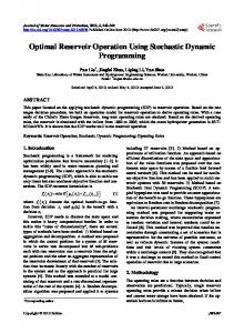
A A2 Ap the cartesian product 1 and a state is one out of n points in this set (State space. Attributes are income, age, and interest. The corresponding attribute values ar).
a = ("low", "midage", "indifferent")
offer wish indifferent
age
final rejection
old n m w i d no teen age low le unk age d i n d com h mi e hig Fig. 1. State space. Attributes are income, age, and interest. The corresponding attribute values are not restricted to those four shown in the figure.
The process of acquiring customers is stochastic by nature. If an action
ut
is
xt
imposed on a customer characterized by dataset , then his reaction, and thus the x t + 1 marketer’s knowledge about him at time , i.e. t + 1 , is usually not uniquely determined. However, for given
xt
and
ut
we can obtain a probability distribution
xt + 1
of by means of statistical experience (or from an expert by rule of thumb). So, the process is considered a time-invariant stochastic system, which leads to Definition 3 The state transition in a process of acquiring customers is governed by a conditional p x x u probability function X t + 1 t t which specifies the probability of attaining x
x
u
state t + 1 from state t and under control t . The goal of the process is to realize the highest profit, which is the difference
U
between income and expenses. Every action i runs up costs. On the other side, income is only realized after the customer signs a contract. In this case, the attribute aip is "final acceptance", which induces Definition 4
= ai1 ai2 aip X i = 1 n The termination set T is the set of states i , , aip T' = X \ T where is "final acceptance". In the following we set . If the process of acquiring customers reaches the termination set it stops. Then, the marketer earns income, whose amount depends on the specific product or business service. For simplicity, we regard one type of product only, that is, e.g. not insurances in general but life insurances. The exact amount of income (e.g. brokerage) is determined by the actual values of some customer attributes, e.g. the level of wage or salary. So the expected income is a function of the terminating state.
Definition 5
The return function r : T R maps each state in the termination set, x T to an expected income value, which usually lies in the compact interval of possible income values R . For x T' we set r x = 0 . Using normalization r is transformed into rmax = maxR x = r x r max r fuzzy goal G with membership function G , where [Bellman, R.E., Zadeh, L.A.: Decision-making in a fuzzy environment. Management Science ]. All actions are subject to constraints resulting from costs, customer characteristics (preferences), or supplementary marketing knowledge. For example, the total cost of actions should be low in order to maximize the potential income. Actions should also fit the customer characteristic and preferences as well as possible with the aim to reach the termination set finally. Since fitness and preference are a matter of degree, we use fuzzy set to represent constraints.
Definition 6
C xt
xt X
over the control space U . u | x u U The membership function of these sets will be denoted by C t t , t . Finally, we turn our attention to finding the sequence of controls that maximize the return function subject to the given constraints. It is denoted optimal policy [Bellman, R.E., Kalaba, R.: Dynamic programming and modern control theory. New York (1]. Since the termination time is unknown in advance, it is convenient to express the controls by a stationary policy function [Kacprzyk, J.: Multistage decision-making under fuzziness. Köln (1983)]. Constraints are state-dependent fuzzy sets
,
Definition 7
x T' A stationary policy function : T' U associates with each state t an input
ut
, which should be applied to the system when it is in state t = 0 1 2 , x t T ' .
xt
, i.e.
ut = xt
,
4 Dynamic Programming under Fuzzy Environment The extension of dynamic programming to multistage decision making under fuzziness was established by Bellman and Zadeh [Bellman, R.E., Zadeh, L.A.: Decision-making in a fuzzy environment. Management Science ]. They introduced the concepts of fuzzy goal, fuzzy constraint and the following idea of fuzzy decision [Bellman, R.E., Zadeh, L.A.: Decision-making in a fuzzy environment. Management Science ][Kacprzyk, J.: Multistage decision-making under fuzziness. Köln (1983)]. Definition 8 G G n C Cm Given n fuzzy goals 1 and m fuzzy constraints 1 in a space of alternatives X . Then, the resultant decision is the fuzzy set D with the D x = G1 x * * Gn x * C1 x * * Cm x membership function for x X * each , where " " is an aggregation (confluence) operator. The maximizing op t decision is defined as x X such that
xopt = max D x xX .
(I have asked the
academic advisor for answering this question. She agreed to my idea.)
Multistage decision-making in a fuzzy environment is usually classified with respect to three aspects [Kacprzyk, J.: Multistage decision-making under fuzziness. Köln (1983)][Kacprzyk, J., Esogbue, A.O.: Fuzzy dynamic programming: Main developments and applica]:
• the type of termination time: fixed and specified in advance, implicitly given by entering a termination set of states, fuzzy, and infinite;
• the type of system under control: deterministic, stochastic, and fuzzy; • the type of aggregation operator: min, product, weighted-sum, max, etc. Here we briefly review Bellman and Zadeh’s approach to decision-making under fuzziness with a fixed termination time in the case of a stochastic system using min-type aggregation operator [Bellman, R.E., Zadeh, L.A.: Decision-making in a fuzzy environment. Management Science ]. Although this case is not appropriate for describing the optimization of process of acquiring customers, it clarifies the relation to classic dynamic programming and the general idea of fuzzy dynamic programming. We have to say that, in contrast to Definition 6 and Definition 7, the fuzzy constraints are stage- dependent and the policy function is not time-invariant. Other approaches to decision-making under fuzziness both for this type and other types of termination time and systems can be found in [Esogbue, A.O., Fedrizzi, M., Kacprzyk, J.: Fuzzy dynamic programming with stochastic syste][Kacprzyk, J.: Multistage decision-making under fuzziness. Köln (1983)][Kacprzyk, J., Esogbue, A.O.: Fuzzy dynamic programming: Main developments and applica]. The system under control can be assumed to be a Markov chain whose temporal p x t + 1 | xt u t evolution is described by a conditional probability ; xt xt + 1 X = 1 n ut U = 1 m x 0 X , ; is an initial state; t = 0 1 N – 1 ; N is fixed and specified. We assume that at each t there
is a fuzzy constraint is imposed on
xN
C t u t
on
ut
N x , t = 0 1 N – 1 , and a fuzzy goal G N
.
u opt u Nopt– 1 The problem is to find an optimal sequence of controls 0 to maximize the probability of realizing the fuzzy goal subject to the fuzzy constraints, i.e.
D u0opt uNopt– 1 | x0 =
max 0 u0 CN – 1 uN – 1 EGN xN u0 uN – 1 C
,
N where the fuzzy goal G is regarded as a fuzzy event in X with probability
E GN x N =
xN X
p xN | x N – 1 u N – 1 GN x N
and thus
D u0opt u Nopt– 1 | x0 = 0 u N – 1 u max N – 1 p x N | x N – 1 u N – 1 G N x N C u0 u N – 1 C 0 xN X
(1)
. Since the two right-most terms depend only upon
D u0opt
opt uN –1
uN – 1
,
can be rewritten as
| x0 = max 0 u0 CN – 2 uN – 2 EGN – 1 xN – 1 u0 uN – 2 C
, GN – 1 xN – 1 = max CN – 1 uN – 1 EGN xN uN – 1 where . On repeating this backward iteration we obtain the set of recurrence equations GN – i xN – i = max CN – i uN – i EGN – i + 1 xN – 1 + 1 uN – i E GN – i + 1 x N – 1 + 1 =
xN – i + 1 X
,
p xN – i + 1 | xN – i u N – i GN – i + 1 x N – i + 1
By solving it, we consecutively obtain u opt = Nopt– i x N – i that N – i .
. uNopt– i
, or, in fact, optimal policies
Nopt– i
such
5 Fuzzy Dynamic Programming for Stochastic System with Implicitly Defined Termination Time We turn now to the case of controlling a stochastic system with implicitly defined termination time, which fits the optimization of acquiring customers stated in Optimization of Acquiring Customers. In the following we introduce an appropriate method for solution of this case. X = 1 k k + 1 n Given , we assume that the termination set T
x T'
n consists of k + 1 and 0 . From Definition 4 we derive easily that C u t | x t 0 xt T ' C u t | x t = 1 x T for , and for t and for arbitrary
ut U
respectively. Furthermore, for the conditional probabilities of a state p x t + 1 | x t u t = 1 u U x = xt T transition under a control t hold if t + 1 , and p x t + 1 | x t u t = 0 x t T xt + 1 xt ut U if , and for every respectively. For a stochastic system with implicitly defined termination time the number of stages from initial state to final one is unknown in advance. In fact, the number N of x T
x T'
stages from an initial state 0 to any final state N is a random variable, x0 u0 u1 uN which depends on , the series of controls , and the corresponding p x t + 1 | xt u t conditional probabilities . u u ut Now we suppose that the sequent inputs 0 1 are determined by a : T' U stationary (time-invariant) policy function (see Definition 7). So, for a
x T' D x certain policy , in a given state t the decision t with respect to the x x policy is the confluence of the constraint in the transition from t to t + 1 , D x C xt and the next decision x + 1 with respect to (see Definition 8). If xt + 1 T x x D x = Gxt + 1 we set t + 1 for arbitrary . Given t , the state t + 1 is a random variable which is characterized by the conditional probability function p x t + 1 | xt u t . Thus
Dxt = Cxt EDxt + 1
or D xt | = C xt | x t ED xt + 1 |
ED xt + 1 | = +
p x t + 1 | x t x t D x t + 1 |
p x t + 1 | x t x t G x t + 1
xt + 1 T' xt + 1 T
and hence
where
(2)
D x t | = C x t | xt
p x t + 1 | x t x t D x t + 1 |
p x t + 1 | x t xt G xt + 1
xt + 1 T'
+
xt + 1 T
which is, in xt n effect, a system of equations (one for each value of ). = 1 k T Let be a policy, its i-th component is a control in state C = C 1 | 1 C k | k T i of system . is a constraint D = D 1 | D k | T vector, is a control vector, while a goal G = G k + 1 G n T vector is . The components of C and D k are the values of the membership function of C and D at 1 respectively. G The components of are the values of the membership function of the fuzzy goal G at the states in the termination set T . We further introduce the k k -transition matrix PT = pij i j = 1 k
and the k n – k -transition matrix PT' = pij i = 1 k
j = k + 1 n
,
whose elements are the conditional probabilities for the state transition pij = p j | i i
(2)provided policy . With these definitions the system of equations in can be converted into a more compact form: (3) D = C PT' D + PT G
where the minimum operator is applied componentwise to the vectors. A policy ' is said to be optimal if and only if ' is better than or not worse | ' D i | '' than any other policy in the policy space, i.e. D i for all '' ' and i = 1 k , which defines a preordering. Using the alternation principle [Bellman, R.E., Zadeh, L.A.: Decision-making in a fuzzy environment. opt Management Science ], it can be easily shown that there exists an optimal policy so that
opt = opt = max D D D .
opt (3)Now we can obtain the following functional equation for the optimal policy from
: (4)
opt = max P opt + P D C T' D T G .
(4)It can be shown easily that the total number r of distinct policy vectors
1 r is finite: Since a policy associates with each state x t T ' an input ut U which should be applied to the system, and T' and U consist of k and m k
elements respectively, we get r = m . Then on using in place of "max", opt = max P opt + P D C T' D T G . becomes Dopt = C 1 PT' 1 Dopt + PT 1 G C r PT' r Dopt + PT r G
(5)
Dopt =
= 1 C r
or
PT' Dopt + PT G
.
(5)Taking advantage of the distributivity of and we can change r Dopt = C PT' Dopt + PT G =1 . into (6)
Dopt =
(6)From
r =1 C
Dopt =
r =1 C
r PT' =1
it can be concluded that the solution of Dopt =
r PT' =1
Dop t
Dopt + PT G
.
Dopt + PT G
.
is the (componentwise) minimum of
r =1 C
and (7)
Dopt =
= 1 PT' r
Dopt + P T G
.
(7)The first equation can be solved directly. For transparency in solution of the := Dopt A := PT' b := PT G second one, we set , , . Then r Dopt = P T' Dopt + P T G =1 .
can be written as =
= 1 A + b r
k + 1 =
,
r A k =1
+ b
0 T , = 0 0 . k The proof line is to show that the series of , k = 0 1 is monotone k + 1 k nondecreasing and bounded from above. We assume that for some k . Using the iteration above, we have
which can be solved by iteration
k + 2 = A1 k + 1 + b 1 A r k + 1 + br A1 k + b1 Ar k + br = k + 1
,
1 0 k + 1 k (7)and noting that , it follows that for k = 0 1 . The series k is bounded from above by = 1 1 . Thus, it converges to the solution of
Dopt =
= 1 PT' r
Dopt + P T G
.
.
6 Conclusion Remarks In this paper we examine the process of gaining customers as a multistage decision process with stochastic state transitions, fuzzy constraints, a fuzzy goal, and an implicitly defined termination time. We present a new model of fuzzy stochastic dynamic programming, which follows Bellman and Zadeh’s concept of fuzzy decision [Bellman, R.E., Zadeh, L.A.: Decision-making in a fuzzy environment. Management Science ]. Since the state space in the model consists of granularized information on customers, it fits the requirements of customer-oriented marketing. The problem of how to choose appropriate marketing actions in order to maximize profit, leads to solve the decision problem by iteration, which yields an optimal policy. Critical discussion of the result and demonstration examples for the above-mentioned model and method will be given in another paper owing to the limitation of space. The task of multistage decision-making arises in a variety of real-world problems. For example, in [Klir, G.J., Yuan, B.: Fuzzy sets and fuzzy logic. Upper Saddle River, New Jersey (1995)], fuzzy dynamic programming is considered as a decision problem regarding a finite-state automaton with fuzzy states and fuzzy inputs. And in [Esogbue, A.O.: Fuzzy dynamic programming, fuzzy adaptive neuro control, and the general me] it is applied to medical diagnosis through a diagnosis decision model. Since many such problems are stochastic in nature and have implicitly defined termination time, we can assert that although the discussed methods are marketing-oriented, they can also be applied to other economic, technical and social problems, which we will turn to in a forthcoming paper.
References 1. Bellman, R.E.: Dynamic programming. Princeton, New Jersey (1957) 2. Bellman, R.E., Kalaba, R.: Dynamic programming and modern control theory. New York (1965) 3. Bellman, R.E., Zadeh, L.A.: Decision-making in a fuzzy environment. Management Science 17 (1970) 4, pp. B-141 - B-164 4. Bundesverband Finanzdienstleistungen e. V. Berlin: FiANTEC Professional & AkquiSys: Moderne Systeme für Kundengewinnung und provisionierten Vertrieb. Finanz Forum & Finanz-Fach-Office: Organ des Bundesverbands Finanzdienstleistungen e. V. Berlin. (1999) 1, p. 13 5. Esogbue, A.O., Fedrizzi, M., Kacprzyk, J.: Fuzzy dynamic programming with stochastic systems. In: Kacprzyk, J., Fedrizzi, M. (Eds.): Combining fuzzy imprecision with probabilistic uncertainty. Lecture Notes in Economics and Mathematical Systems 310. Berlin (1988) 6. Esogbue, A.O.: Fuzzy dynamic programming, fuzzy adaptive neuro control, and the general medical diagnosis problem. Computers and Mathematics with Applications 37 (1999), pp. 37-45 7. Kacprzyk, J.: Multistage decision-making under fuzziness. Köln (1983) 8. Kacprzyk, J., Esogbue, A.O.: Fuzzy dynamic programming: Main developments and applications. Fuzzy Sets and Systems 81 (1996), pp. 31-45. 9. Keppler, M.: Wirksame Verkaufsförderung durch psychologische Kundensegmentierung. Thexis. (1993) 2, pp. 20-23 10. Klingsporn, B.: Teilmärkte bilden: Yuppie oder Skippie - wer ist ihr Kunde? Bank Magazin. (1996) 7, pp. 34-42 11. Klir, G.J., Yuan, B.: Fuzzy sets and fuzzy logic. Upper Saddle River, New Jersey (1995) 12. Küspert, A.: Bildung und Bewertung strategischer Geschäftsfelder. Die Bank. (1991) 8, pp. 425-434 13. Küspert, A.: Kundengruppenbildung im Privatkundengeschäft von Kreditinstituten - eine Fallstudie. Zeitschrift für Bankrecht und Bankwirtschaft. (1992) 3, pp. 184-201 14. Link, J., Hildebrand, V.: Database Marketing und Computer Aided Selling. München (1993) 15. Seyfarth, H.: Erfolgsorientierte Akquiseplanung. Technik & Gesellschaft. 2 (1998) p. 36 16. Swoboda, U.: Erfolgsfaktoren der Konsumentenbanken. Finanzierung, Leasing, Factoring. (1996) 3, pp. 89-91 17. Weber, R.: Verborgene Potentiale aufdecken. Bank Magazin. (1994) 9, pp. 44-46 18. Zadeh, L.A.: Some reflections on soft computing, granular computing and their roles in the conception, design and utilization of information/intelligent systems. Soft Computing. 2 (1998) 1, pp. 23-25