Stochastic Epidemiologic Modeling Using a Microcomputer ...

Preventive Veterinary Medicine, 5 (1988) 159-168

159

Elsevier Science Publishers B.V., Amsterdam - - Printed in The Netherlands

Stochastic Epidemiologic Modeling Using a Microcomputer Spreadsheet Package TIM E. CARPENTER

Department of Epidemiology and Preventive Medicine, School of Veterinary Medicine, University of California, Davis, CA 95616 (U.S.A.) (Accepted for publication 22 June 1987 )

ABSTRACT Carpenter, T.E., 1988. Stochastic epidemiologic modeling using a microcomputer spreadsheet package. Prey. Vet. Med., 5: 159-168. A stochastic epidemiologic simulation model was created using a microcomputer spreadsheet package. The model (III) simulated a modified Reed-Frost model. The modifications were (1) vaccination was permitted in the population, (2) vaccinal immunity waned and was random and (3) the number of effective contacts varied randomly among periods. The methodology presented in this paper should enable the reader to recreate this or other stochastic simulation models. Sample output results were reported to illustrate the potential use of stochastic epidemiologic modeling using a spreadsheet package.

INTRODUCTION

Epidemiologic modeling is a technique which may help the epidemiologist understand complex disease processes, predict epidemic patterns and evaluate intervention strategies. Until recently, however, it has required the user to be a skilled computer programmer either with access to a large expensive computer or with a significant time commitment. Both of these constraints have made epidemiologic modeling unattractive to all but a few epidemiologists and mathematicians. These constraints may now be overcome, if the modeler has basic mathematic and computer skills, by using one of several spreadsheet packages available for relatively inexpensive microcomputers. Earlier spreadsheet models (referred to as I and II in (Carpenter, 1984), although easy to construct had the limitation that they could only be used to evaluate the average outcome of an epidemic, i.e. they were deterministic. As Bailey stated, "It is the essential failure of [such] deterministic models to square with the facts that has led to their abandonment in many quarters and consequent replacement by corresponding probability, or stochastic, represen0167-5877/88/$03.50

© 1988 Elsevier Science Publishers B.V.

160 tations" (Bailey, 1975, p. 12 ). Although it is recommended that an initial model be as simple as possible, if and when it fails to satisfactorily simulate a problem, a more complex, stochastic approach may improve the model. A stochastic model generates several results, which may be used to calculate the mean, standard deviation and range of outcomes for a single system. While a stochastic model is more epidemiologically informative than the deterministic version, it also complicates the mathematical analysis. "These complexities appear to result largely from the introduction of transition probabilities that are quadratic functions of the basic random variable, rather t h a n merely linear functions as with m a n y of the commoner, and relatively tractable, birth-and-death processes" (Bailey, 1975, p. 42). Simulation models may be used to mimic these complex stochastic processes with the use of random numbers generated to represent appropriate frequency distributions. A model (referred to as III in this report) was developed and random numbers generated to (1) demonstrate the construction of a stochastic simulation model using a spreadsheet format and (2) evaluate, using the simulation results, the effect of different vaccination rates on an epidemic pattern. ANALYTIC METHODS

Electronic spreadsheet A spreadsheet package, SuperCalc3, release 2.1 (Sorcim Corporation, San Jose, CA ) was used for the construction and simulation of the model. A spreadsheet may be thought of as an accountant's columnar pad combined with a calculator and pencil. It provides the user with a worksheet where he or she can enter text or labels, data and mathematic or trigonometric equations. It performs calculations as indicated and given any change in information it will automatically perform recalculations without mathematical errors. The potential worksheet of the spreadsheet used in this example has up to 9999 rows and 127 columns (1 269 873 cells) available. Single equations, labels or data are stored in cells identified as the intersection of a row and a column, e.g. A1 refers to a cell whose location is the first row of Column A.

Classic Reed-Frost model The basic assumptions of the classic Reed-Frost model (Abbey, 1952) were used to construct the initial simulation model. The following equations were used to construct the model: C~+1 =St" (1 _qC,) where t = the time period, Ct+ 1= the number of infectious cases in time period

161 t + 1, St = the number of vaccinated and non-vaccinated susceptible individuals in time period t, and q=l-p where p = the probability of one specific individual making effective contact with another given individual which would result in an infection if one were infectious and the other susceptible. Thus, q is the probability of an individual avoiding such a contact. Furthermore, p is calculated as p=k/(n-1) where k = the number of effective contacts made by an individual during one time period (t) and n = the population size. The spreadsheet codes used to construct the classic Reed-Frost model were described in an earlier paper (Carpenter, 1984). The number of susceptibles in a given time period is calculated as those individuals which were susceptible in the previous time period and did not become infected St+l = S t - C t + l Modified Reed-Frost model Model III is a modification of the classic Reed-Frost model. Modifications of the classic model were as follows: Model III included a control component, vaccination; duration of vaccinal immunity was assumed to vary from 6 to 2 weeks, be stochastic and have a negative exponential distribution; individual immunity could be identified and susceptibles vaccinated; number of effective contacts varied among time periods and were normally distributed. Susceptibles were divided into two groups, vaccinated and non-vaccinated. The number of vaccinated susceptibles in a given time period was calculated as the number of non-vaccinated susceptibles which were vaccinated in the previous time period and did not become infected during the period when they were vaccinated. It was assumed that since there was random mixing, newly vaccinated and non-vaccinated susceptibles were equally likely to become a new case in the subsequent period. The equation used to calculate the number of vaccinated susceptibles was as follows: VSt+, = [ N S t - C t + l " ( N S t / ( VSt + N S t ) ) ] "vr where V S - - the number of vaccinated susceptibles, N S = the number of nonvaccinated susceptibles, N S t / ( VSt + N S t ) = the proportion of non-vaccinated susceptibles in the susceptible population and vr-- the vaccination rate, or proportion of non-vaccinated susceptibles vaccinated per week. The model there-

162 fore assumed that complete herd or flock vaccination was not feasible in a single time period. Furthermore, it was assumed that vaccination efficacy was 100%. Modifications to these assumptions could easily be made to conform to other situations, e.g. vaccination performed in a single time period or vaccination efficacy < 100%. The number of non-vaccinated susceptibles in a given time period was calculated similarly to the vaccinated susceptibles, except ( 1 - v r ) was substituted for vr, to calculate the proportion of non-vaccinated susceptibles in the previous period which did not become infected and were not vaccinated N S t + 1 = [ N S t - Ct+l" ( N S t / ( VSt + N S t ) ) ]" (1 - vr)

Vaccinal immunity was assumed to last for 6, 5, 4, 3 or 2 weeks with a negative exponential distribution, i.e. the proportion of non-infected vaccinated individuals having a 6-week immunity was exponentially greater t h a n those with a 5-week immunity which was exponentially greater t h a n those with a 4week immunity, etc. This relationship continued until all vaccinated individuals which did not have a 3- to 6-week immunity were assumed to have a 2week immunity. The equation used to determine the population of 6-week vaccinated immune individuals ( V I ( 6 ) ) was V I ( 6 ) t + ~ = V S t - ( C t + 1 . ( V S t / ( V S t -it- N S t ) ) ) .e -u~

where Ui is the ith uniform deviate. Alternative vaccinal immune populations were calculated using the same formula after first excluding individuals which were included in the previous vaccinal immune categories, i.e. the 5-week vaccinal immune population excluded those with a 6-week immunity, the 4-week vaccinal i m m u n e population excluded those with either a 6- or 5-week vaccinal immunity, etc. In this way a negative exponential distribution was generated for vaccinal immunity as described above. Acquired immunity was assumed to be wholly conferred and calculated as the sum of all individuals previously infected AIt+l =Ct + Alt

where A I = acquired immune. A list of the variables, their location in the spreadsheet and their descriptions appear in Table I. Spreadsheet coding of the equations into spreadsheet format (Table II ) was performed as described in an earlier paper ( Carpenter, 1984 ). Incidence and prevalence of vaccinal immunes were calculated for each of the vaccinated immune categories. Incidence information was used to determine the duration of immunity for each individual. Prevalence information was used to verify the model and calculate total population size. Implementation of a stochastic element in this model was simplified by using the spreadsheet's random number generator. A random generator equation

163 TABLE I Epidemiologic model variables and their spreadsheet locations Column (s) location

Variable and description

A-F G H I J K L M N 0 P Q R S T U V W X Y Z AA

Uniform deviates (6) Time: ranges from i to 20 weeks Cases Vaccination rate: assumed constant once specified in cell I3 Susceptibles (vaccinated) Susceptibles (non-vaccinated) Susceptibles (total) Vaccinal immune (incidence): 6 weeks Vaccinal immune (prevalence): 6 weeks Vaccinal immune (incidence): 5 weeks Vaccinal immune (prevalence): 5 weeks Vaccinal immune (incidence): 4 weeks Vaccinal immune (prevalence): 4 weeks Vaccinal immune (incidence) : 3 weeks Vaccinal immune (prevalence): 3 weeks Vaccinal immune (incidence) : 2 weeks Vaccinal immune (prevalence): 2 weeks Acquired immune: immunity is wholly conferred Total population Contacts: mean is specified in cell Y3 p: probability of making an effective contact q: probability of avoiding an effective contact

is presented in Appendix i for users of programs which do not have this feature built in. SAMPLE OUTPUT RESULTS

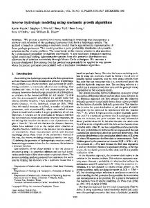
The model was constructed using a 24 X 27 matrix ( 24 rows and 27 columns) spreadsheet and required 9K bytes of memory. The operation time simulating 20 time periods was approximately 3 s. The current spreadsheet utilized the computer's m a t h coprocessor which significantly reduced the run time of previously reported models. Three hundred and fifty simulation runs, 50 at each of seven vaccination rates (0, 20, 30, 50, 70, 80 and 100% ) were performed. At the no or high ( > 70% ) vaccination rates, a high proportion of epidemics ended quickly, i.e. before completion of the 20 weeks (Fig. 1). At low vaccination rates (20, 30 and 50% ), epidemic duration was typically long ( > 20 weeks). The epidemic pattern also varied with assumed vaccination rate. At extreme vaccination rates, 0 and 100%, epidemics were unimodal, peaking and termi-

164 T A B L E II Initial populations a n d spreadsheet coded equations for the epidemic simulation of a stochastic, vaccination model A

B

C

D

E

F

G

H

Cases

1 2

Pseudorandom number generator calculations

3

Uniform 1

Uniform2

Uniform3

Uniform4

Uniform5

Uniform6

Time

4

RAN

RAN

RAN

RAN

RAN

RAN

i

1

2

IF(H4 < 1,0, (J4 + K4) • (1 - AA4 ^ H4))

5

6

I

J

1 2

Vaccination rate Rate=I3

Susceptible population

3 4 5 6

0.8 IF(I3 = 1,0.999999,I3) IF(I3 = 1,0.999999,I3)

Vaccinated susceptibles 0 I F ( ( K 4 - H5* (K4/L4)) > 0 , ( K 4 - H5* (K4/L4))* I4,0)

K

L

Susceptible population

Vaccinated immunes Total susceptibles J4+K4 J5+K5

Non-vaccinated susceptibles 1000 IF((K4 - H 5 , (K4/L4)) > 0, (K4 - H5 * (K4/L4)) • (1 - I4),0) IF( (K5 - H6* (K5/L5)) + (O 1 + Q2 + $3 + U4) > 0, (K5 - H6* (K5/L5)) * (1 - I5) + (01 + Q2 + $3 + U4),0) I F ( ( K 6 - H T , (K6/L6)) + (M1 + 0 2 + Q 3 + S 4 + U 5 ) > 0, ( K 6 - H7* (K6/L6))* ( 1 - I6) + (M1 + O2 + Q 3 + $4 +U5),0)

M 1 2 3 4 5 6

Vaccinated immunes 6 weeks Incidence IF(J3- H 4 * (J3/L3) > 0, (J3- H 4 * (J3/L3))* E X P ( - C4),0) I F ( J 4 - H 5 * (J4/L4) > 0, (J4 - H 5 * (J4/L4)) * E X P ( - C5),0)

N

Prevalence 0 SUM(MI:M5)

0 Vaccinated immunes 5 weeks Incidence IF(J3 - H 4 * (J3/L3) - M 4 > 0, (J3- H 4 * (J3/L3)- M 4 ) * E X P ( - D4),0) IF(J4- H 5 * (J4/L4) - M 5 > 0, (J4 - H 5 * (J4/L4) - M 5 ) * E X P (- D5),0)

165

P

Q Vaccinated immunes 4 weeks Incidence IF(J3 - H4* (J3/L3) - (M4 + 04) > 0,(J3 - H4 * (J3/L3) - (M4 + 04)) * EXP( - E4),0)

1 2 3

Prevalence

4 5

0 SUM(01:05)

6

R 1 2 3 4 5

S

Prevalence SUM(QI:Q4)

Vaccinated immunes 3 weeks Incidence

IF(J3-H4*(J3/L3)-(M4+O4+Q4)>O,(J3-H4*(J3/L3)-(M4+O4+Q4))*EXP(-F4),O)

6

T

U

Prevalence SUM(S2:S4)

Vaccinated Immunes 2 weeks Incidence IF(J3 - H4 * (J3/L3) - (M4 + 0 4 + Q4 + $4) > 0,J3 - (H4* (J3/L3) + M4 + 0 4 + Q4 + $4),0)

1 2

3 4 5 6

V 1

X

Immunes

2 3 4 5 6

1 2 3 4 5 6

W

Prevalence

Acquired

SUM(U3:U4)

0 H4 H5+W5

Total H4+J4+K4+N4+

P4+R4+T4+V4+W4

H5+J5+K5+N5+P5+R5+T5+V5+W5 H6+J6+K6+N6+P6+R6+T6+V6+W6

y

Z

AA

Contacts U3 = mean 6 Y3 + 1. ( S Q R T ( - 2-LN(A4))* COS(2"PI'B4)) Y3 + 1 * ( S Q R T ( - 2.LN(AS))*COS(2"PI'BS)) Y3 + 1. ( S Q R T ( - 2.LN(A6))* COS(2"PI'B6))

P Y4/(X4-1)

q 1 - Z4

Numbers on the left hand side refer to row No. Column headings Nos. identify the population variables and are used in the coded equations of the epidemic simulations.

166 1 O0

~,s0~oo 60

r

0 c~

5~

~ 40

"~

y

"5 >

0~ 0

2'0

40

8'0

6'0

Epidemics (%) > 20 weeks Fig. 1. Percentage of epidemics, by vaccination rate, lasting longer than 20 weeks.

nating early as discussed above. The epidemic pattern associated with low vaccination rates, 20 and 30%, was bimodal with peaks occurring at 5 and 13 weeks (Fig. 2 ). The number of cases at the first peak was significantly larger than at

250

v.r. = 2 0 % ---x--- v.r. = 3 0 % v.r. = 5 0 %

200

u

+

v.r. = 7 0 %

+

v.r. = 8 0 %

150

z]

E

too

Z

50

0

5

10

15

20

Time (weeks) Fig. 2. Epidemic curves of epidemic simulation model assuming different vaccination rates (v.r.).

167 the second. Higher vaccination rates were associated with 3 peaks i n the 20week period and simulated a cyclic pattern with peaks occurring approximately at weeks 4, 13 and 20. These sample results represent a small fraction of the potential to which the epidemiologist can have access with the aid of spreadsheet modeling. Although useful, deterministic models are sometimes constraining in that they do not permit a realistic evaluation of patterns of disease. Since individuals differ, it is sometimes necessary to incorporate these differences into a simulation model. The methodology presented in this paper should permit the user to simulate a variety of disease examples which are enhanced with a stochastic element and parameters, e.g. immunity, latency or infectious periods, using a variety of distributions. PROGRAM AVAILABILITY Model III may be constructed by following the instructions presented in this paper. Although the graphics capability and speed are specific to a particular spreadsheet, similar results may be obtained from the more than 50 spreadsheets currently available. ACKNOWLEDGMENTS This study was funded in part by a grant from the Livestock Diseases Research Laboratory, University of California, Davis. APPENDIX I Random number generation

As described by Ralston and Reilly (1983), "A random-number generator is a computer procedure which scrambles the digits of an integer to produce a new integer... The idea is to produce a sequence of integers which, in spite of being produced by a fixed procedure, will serve as random variables in computer simulations..." (Ralston and Reilly, 1983, p. 1260). A random number with a uniform distribution, or uniform deviate, was generated using the arithmetic function (RAN) provided in the spreadsheet package. An algorithm which may be used to generate a uniform deviate is presented below for use with spreadsheets which do not have the random number generator function available. A random number generator, Xn+ 1= (aXn-[- C) mod m, may be created following the principles presented by K n u t h (1969): (1) a seed (Xn) is selected using a table of random numbers; (2) m is large and is conveniently taken as the computer's wordsize (216--65536, for a 16-bit computer), such that

168

m > Xo,a,c; (3) a m o d 8-- 5, w h e n using a b i n a r y b a s e d c o m p u t e r ; (4) a > m 1/2, a > m/100, b u t a < rn - m 1/2 ( t h e value a = 25173 m e t t h e s e c r i t e r i a ) ; (5) c is a n odd n u m b e r a n d selected so t h a t c/m~0.2113249, t h u s c = 1 3 8 4 9 , and; (6) X,+ 1/m is a r a n d o m n u m b e r w i t h a u n i f o r m distribution. T w o a d d i t i o n a l r a n d o m n u m b e r distributions, n o r m a l a n d negative expon e n t i a l were s i m u l a t e d a c c o r d i n g to t h e following formulas: (1) n o r m a l deviate (Xi) ( B o x a n d Muller, 1958, p. 611 )

Xi= ( - 2 lnUli) 1/2 cos 2piU2i w h e r e U1 a n d [72 are a p a i r of u n i f o r m deviates a n d Xi has m e a n zero a n d u n i t variance. ( 2 ) negative e x p o n e n t i a l deviate ( Schreider, 1966, p. 316 ) :

Xi = - I n ( l -

Ui)

REFERENCES Abbey, H., 1952.An examination of the Reed-Frost theory of epidemics. Human Biol., 24: 201-233. Bailey, N.T.J., 1975. Historical outline. In: The Mathematical Theory of Infectious Diseases. Hafner Press, New York. Box, G.E.P. and Muller, M.E., 1958. A note on the generation of random normal deviates. Ann. Math. Stat., 29: 610-611. Carpenter, T.E., 1984. Epidemiologic modeling using a microcomputer spreadsheet package. Am. J. Epidemiol., 120: 943-951. Knuth, D.E., 1969. Random numbers. In: The Art of Computer Programming. Reading, MASS: Addison-Wesley, pp. 1-160. Ralston, A., Reilly Jr., E.D., (Editors), 1983. Random number generation. In: Encyclopedia of Computer Science and Engineering. 2nd edn. Van Nostrand Reinhold, New York, p. 1260. Shreider, Y.A., 1966. The Monte Carlo Method. Pergamon Press, New York, p. 316.