European Water 60: 299-306, 2017. © 2017 E.W. Publications
Stochastic generation of low stream flow data of Perigiali Stream, Kavala city, NE Greece T. Papalaskaris1* and T. Panagiotidis2 1
Department of Civil Engineering, Democritus University of Thrace, Kimmeria Campus, 67100 Xanthi, Greece Department of Mechanical Engineering, Eastern Macedonia & Thrace Institute of Technology, 65404 Kavala, Greece * e-mail:
[email protected] 2
Abstract:
The present study generates synthetic low stream flow time series of an entire calendar year considering the stream flow data recorded during two certain interval periods of the years 2016 and 2017. We examined the goodness of fit tests of six theoretical probability distributions to low stream flow data acquired at the exit of the Perigiali stream, Kavala city, NE Greece watershed, during part of May, June, July, part of August, part of December 2016 and part of January 2017, using either a combination of a 3-inches U.S.G.S. modified portable Parshall flume in conjunction with a 3-inches Montana portable flume and a combination of a 3-inches conventional portable Parshall flume in conjunction with a 3-inches Montana portable flume and calculated the corresponding probability distributions parameters. The six specific probability distributions used in this study were the following: (1) Gumbel min (Minimum Extreme Value Type 1) distribution, (2) 3-Parameter Log-Normal distribution, (3) Pearson Type 5 distribution, (4) Pearson Type 6 distribution, (5) Two-Parameter Weibull distribution and (6) Wakeby distribution. The Kolmogorov-Smirnov, Anderson-Darling and Chi-Squared, GOF tests were employed to show how well the probability distributions fitted the recorded data and the results were demonstrated through interactive tables providing us the ability to effectively decide which model best fits the observed data.
Key words:
artificial time series, discrepancy ratio, goodness-of-fit tests low flow data, conventional and modified Parshall flumes
1. INTRODUCTION Artificial stream flow time series generation is a means of paramount importance in hydrology and water resources management in order to handle efficiently precarious or doubtful situations, pertinent to a natural watercourse’s flow regime, associated particularly to a short period of stream flow rate data acquisition. The increasing water demands worldwide, caused primarily by the global population increase and exacerbated by the water scarcity due to the climate change, especially in North-Eastern Europe, gives significant prominence to the wise use of the available water resources, showcasing stream flow rate monitoring as a factor of paramount importance with the view to design water storage reservoirs and other water resources management infrastructure works. Therefore, the necessity to minimize dubiety and ambivalence in estimating the flow regime of a natural watercourse constitutes a challenging task in the sector of hydrology and water resources management. This difficulty can only be adequately worked out employing artificial stream flow time series generation procedures and techniques, as a common process.
2. LITERATURE REVIEW Numerous studies and reviews have been carried out in the field of low flows, handling different subjects such as the fit of theoretical probability distribution functions on observed low stream flow rate data, surface runoff and groundwater exchange relationships, watershed drought management, hydrological low-flow and drought indices estimation, watershed water budget and balance compilation, evapotranspiration estimation, daily stream flow variation computations, in-stream environmental stream flows calculation etc. (Matalas, 1963; Beard, 1968; Singh and Stall, 1973;
300
T. Papalaskaris & T. Panagiotidis
Singh, 1987; Vogel and Kroll, 1989; Ming-Ko and Kai, 1989; Vogel and Kroll, 1990; Vogel and Wilson, 1996; Wang, 1997; Smakhtin and Toulouse, 1998; Young et al., 2000; Smakhtin, 2001; Stahl, 2001; Spangler, 2001; Zaidman et al., 2002; Acreman and Dunbar, 2004; Laaha and Blöschl, 2005; Yongqin et al., 2006; Černohous and Šach, 2008; Tallaksen and Hewa, 2008; Gribovszki et al., 2008; Nalbantis, 2008; Gribovszki et al., 2010; Sen and Niedzielski 2010; Demirel et al., 2013; Orlowski et al., 2014; Wittenberg, 2015; Yürekli et al., 2005; Büyükkaraciğan, 2014; Papalaskaris and Panagiotidis, 2016).
3. MATERIALS AND METHODS 3.1 Study area The stream flow rate gauging station, which was established in Kavala city area, a coastal city, located at the north of the Aegean Sea, across the Thassos Island, and surrounded by the Lekani mountain series branches to the North and East and the Paggaion Mountain ramifications to the West, (established in the proximity of the city urban web center and at the eastern exit of the city as well), located at the specific co-ordinates 40°56΄727΄΄ N and 24°25΄929΄΄ E, Perigiali city area, and operated continuously, spanning two individual between each other time interval period from 14.05.2016 to 30.08.2016 and 24.12.2016 to 05.01.2017, as illustrated in Figure 1.
Figure 1. 3-inches U.S.G.S. modified portable Parshall flume gauging station, Perigiali area, Kavala city, Greece (source: Google Earth).
3.2 Sample collection and data used in this study A total number of 203 individual stream flow rate (discharge) measurements were performed within 109 consecutive days, between 14.05.2016 and 30.08.2016 and a total number of 13 individual stream flow rate (discharge) measurements were performed within 13 consecutive days, 24.12.2016 to 05.01.2017, during which a thorough presentation of the methodology and procedure
European Water 60 (2017)
301
followed up was analytically supplied, whereas, all of them were recorded and uploaded on the first author’s personal Youtube platform web-site, namely, “Thomas Papalaskaris”. The first stream flow rate (discharge) measurement (14.05.2016) lasted 1 hour sharp and the last one (30.08.2016), respectively, 48’:01”, as far as the first stream flow rate measurements set time interval is concerned. The first stream flow rate (discharge) measurement (24.12.2016) lasted 1 hour sharp and the last one (05.01.2017), respectively, 48’:01”, as far as the first stream flow rate measurements set time interval is concerned. In accordance with the recorded observations of the only available private meteorological station located at Dexameni area, Kavala city, Greece, Kavala city received total monthly rainfalls as following: 56.80 during May 2016, 14.00 mm during June 2016, 1.60 mm during July 2016 and 10.40 mm during August 2016 (82.80 mm in total respecting the four months) respectively. The recorded stream flow rate (discharge) (denoted by the blue-colored continuous line) and the observed rainfall (denoted by the red-colored vertical bars) during the time period 14.05.2016 and 29.08.2016 are simultaneously illustrated within Figure 2.
Figure 2. Recorded stream flow rate at Perigiali area, 3-inches U.S.G.S. modified Parshall flume, gaging station vs. observed rainfall at Dexameni area station, Kavala city, Greece (source: first author’s personal archive and https://www.meteokav.gr).
3.3 Sample analysis and checking the goodness of fit Mathwave EasyFit and StatAssist software packages was employed to estimate the best probability distribution (based on the Anderson-Darling, Chi-Squared and Kolmogorov-Smirnov goodness-of-fit criteria tests), together with the associated parameters, fitting the daily lowest stream flow data, as well as the goodness-of-fit of all the other candidate probability distributions. Moreover, after having calculated the parameters of the examined probability distributions, we generated a sequence of high quality random numbers for each individual candidate probability distribution with the same parameter values to the origina calculated ones. The KolmogorovSmirnov test (KS-test) tries to determine if two datasets differ significantly, whilst, it has the
302
T. Papalaskaris & T. Panagiotidis
advantage of making no assumption about the distribution of the data (technically speaking it is non-parametric and distribution free). MS Excel software is employed in order to plot the real observed (recorded) against the artificial (generated, forecasted) low stream flow rate (discharge) data. The calculation of six examined candidate probability distribution estimates are of paramount importance as they enable us, by assigning different specified scores, according to their goodness of fit performance, to evaluate which is the most appropriate one simulating the recorded stream flow rate values. The goodness of fit tests are performed in order to evaluate which distribution fits to the low stream flow rate (discharge) data series in the best possible way. The values of AndersonDarling statistics, Chi-square (χ2), Kolmogorov-Smirnov (D) respectively are computed and illustrated within Τable 2, for the entire low stream flow rate (discharge) time series data. It should be underlined that, employing an improvised scoring system, the superscript number makes reference to the order ranking of the probability distribution which best fits the low-flow time series data, ranging from 1 (the best one) to 3 (the worst one). Further, the ranking score values of numbers 3, 2, and 1, are, inversely assigned to the already given, (as above mentioned followed procedure), ranking scores 1, 2, and 3 correspondingly, in order to assess the highest final goodness of fit score obtained for each candidate individual probability distribution, determining, as an outcome, the best one which best fits the observed low stream flow rate (discharge) time series data. Table 1. Goodness of fit tests results for the 3-inches U.S.G.S. modified portable Parshall flume, Perigiali area, Kavala city Greece, gauging station, data series (source: EasyFit, Goodness of Fit). Probability distribution Gumbel min (2P) Log-Normal (3P) Pearson type 5 (3P) Pearson type 6 (3P) Weibull (2P) Wakeby (5P)
Anderson Darling 18.08300 0.5607002 0.4711401 0.6190003 0.764610 4.119200
Perigiali Gauging Station (Goodness of fit types) Kolmogorov Highest final goodness Chi - Squared Smirnov of fit score obtained N/A 0.272100 9.692300 0.089250 2 3.2335002 0.0855803 6 3 9.641300 0.093730 2 3.2045001 0.0649102 5 N/A 0.0506101 3
It can be identified from Table 1, that all the examined probability distributions can be accepted to fit to the low stream flow rate (discharge) time series data at the significant level α of 0.05, except Gumbel min. (2P) and Wakeby (5P) probability distributions, based on the Chi-squared goodness of fit test, whilst, at the same time, based on all three individual goodness of fit tests, Pearson type 5 (3P) obtained the highest score of six. Still, the probability density function of Wakeby (5P) probability distribution (which obtained the highest score based on the Kolmogorov Smirnov goodness of fit test) is finally chosen in order to produce artificial low flow time series data. Visually inspecting the Figure 3, where the real observed (recorded) low stream flow rate (discharge) time series data are plotted against the artificial ones, for the same time period (14.05.2016-29.08.2016) we can identify that both, by first sight, coincide (for the most of the paired values) remarkably well. 3.4 Hydrodynamic methods and equipment for sample data collection and analysis Due to the extremely shallow waters, in conjunction with the extremely low water stream flow velocity prevailing at the gauging station, it is impossible to implement the area-velocity method in order to assess the stream flow rate (discharge), using a current meter mounted on a wading rod, owing to the fact that there isn’t available depth to submerge the current meter as well as the extremely low water stream flow velocity is not sufficient enough to trigger the operation of a current meter; Under those particular circumstances the only alternatives are the use of either a small-sized portable weir plate or a small-sized flume which, eventually, was our final selected
European Water 60 (2017)
303
option, more specifically, a “3-inch U.S.G.S. Modified Portable Parshall Flume”, constructed by means of sea plywood, covered with a sprayed thin smooth polyester coating similar. to that the industry usually covers the outside surface of high developing speed sea vessels, in order to reduce the friction between the outside area of those sea vessels and the sea water, thus ensuring that the friction developed between the bottom as well as the walls of the Flume are minimized to a minimum (Johnson, 1963; Rantz, 1982).
Figure 3. Plot of observed against artificial low stream flow rate time series data for 3-inches modified ortable Parshall flume gauging station, Perigiali area, Kavala city, Greece (Source: Author’s plot compilation).
5. COMPARISON BETWEEN CALCULATED AND SITE-MEASURED LOW STREAM FLOW RATE (DISCHARGE) VALUES The comparison between calculated and site-measured values of low stream flow rates (discharges) is made on the basis of several statistical criteria such as, root mean squared error (R.M.S.E.), relative error (R.E.), efficiency coefficient (E.C.), linear correlation coefficient (r), determination coefficient (r2) and discrepancy ratio (D.C.) (Nash and Sutcliffe, 1970; Krause et al., 2005), as depicted within Table 2. The plot depicted within Figure 4 represents the discrepancy ratio concerning Perigiali Stream, Kavala city, North-Eastern Greece, during the time period between 14.05.2016 and 29.08.2016. At this point, it should be noted that both coordinate axes are in logarithmic scale; therefore, the equations y=x, y=0.5x and y=2.0x are represented graphically by parallel straight lines. In general, the obtained values of the statistical criteria R.M.S.E., R.E., E.C. for Perigiali Stream 3-inches U.S.G.S. modified portable Parshall flume can be considered fairly satisfactory considering the low stream flow rate numerical values. Additionally, the degree of linear dependence between calculated and measured bed load transport rate is very weak, implying that more iterations should be carried out until an artificial low stream flow rate time series data which best fits (by the perspective of the overall achieved statistical efficiency criteria) the observed low stream flow rate time series data is generated.
304
T. Papalaskaris & T. Panagiotidis
Table 2. Statistical criteria values of 3-inches U.S.G.S. modified portable Parshall flume gauging station Perigiali Stream, Kavala city, Greece, (14.05.2016-29.08.2017) (source: authors’ plot compilation archive) Number of paired values 108
RMSE [kg/(m s)] 0.3983
RE (%) -0.8155
EC
r
r2
-0.5490
-0.0133
0.0002
Discrepancy ratio 0.5000
Figure 4. Discrepancy ratio plot of observed against artificial low stream flow rate time series data for Parshall flume gauging station, Perigiali area, Kavala city, Greece (14.05.2016-29.08.2016) (source: authors’ plot compilation).
The above mentioned statistical criteria values concerning Perigiali Stream, Kavala city, NorthEastern Greece, are listed within Table 4. It is noted that the relative error value depicted within Table 4 represents the average value of the relative errors calculated for each pair of calculated and measured bed load values.
5. RESULTS AND DISCUSSION A total number of 203 individual stream flow rate (discharge) measurements were performed within 109 consecutive days, between 14.05.2016 and 29.08.2016, at the Perigiali area, Kavala city, north eastern Greece, at the exit of the homonymous watershed and main stream channel by means of a “3-inch U.S.G.S. Modified Portable Parshall Flume”. The daily lowest flows were undergone a probability distribution analysis and six candidate probability distributions were fitted to the low stream flow rate time series data proving that the Pearson type 5 (3P) probability distribution best fitted the data based on three different goodness of fit tests. As normally anticipated the stream flow rate (discharge) observed early in the morning, late in the evening and during the night patrols were (due to decreased evapotranspiration rate, stemming from the relatively lower temperature, solar radiation and dry wind intensity values hitting, in turn, the entire Perigiali area watershed) relatively higher that those performed around mid-day hours and early in the evening.
6. CONCLUSIONS - FUTURE RESEARCH Perigiali watershed and main stream channel can sustain extremely low flow conditions which
European Water 60 (2017)
305
are essential for low flow studies in order to compile an as much consistent watershed and drought management plan and bridge the research and knowledge pertinent to the south eastern part of Europe were, as generally admitted, only a few stream flow rate (discharge) measurement gauging stations exist and transfer the acquired knowledge to ungauged watersheds as well, in accordance to the suggestions of the Braunschweig Declaration. Furthermore, Perigiali Mediterranean watershed could be proposed to be incorporated within the global network of long-term small hydrological scientific research basins network the importance of which has been worldwide acknowledged. More future stream flow measurements would contribute to the production of extended stream flow rate (discharge) time series data which are of paramount importance in hydrology in order to compile accurate, consistent and sustainable watershed balance and budget computation and drought management plans compilation.
REFERENCES Acreman M. and Dunbar M.J. (2004). Defining environmental river flow requirements – a review. Hydrology and Earth System Sciences, 8(5), 861-876. Beard L. (1968). Simulation of Daily Streamlow. United States Corps of Engineers, Institute of Water Resources - Hydrologic Engineering Centre, Technical Paper 6 (TP-6), Davis. Büyükkaraciğan N. (2014). Determining the best fitting distributions for minimum flows of streams in Gediz Basin. International Journal of Environmental, Chemical, Ecological, Geological and Geophysical Engineering, 8 (6), 417-422. Černohous V., and Šach F. (2008). Daily baseflow variations and forest evapotranspiration. Ekológia (Bratislava), 27(2), 189-195. Demirel M.C., Booij M.J. and Hoekstra A.Y. (2013). Impacts of climate change on the seasonality of low flows in 134 catchments in the River Rhine basin using an ensemble of bias-corrected regional climate simulations. Hydrology and Earth System Sciences, 17 (10), 4241-4257. Gribovszki Z., Kalicz P., Kucsara M., Szilágyi J. and Vig P. (2008). Evapotranspiration calculation on the basis of the riparian zone water balance. Acta Silvatica & Lignaria Hungarica, 4, 95-106. Gribovszki Z., Szilágyi J. and Kalicz P. (2010). Diurnal fluctuations in shallow groundwater levels and streamflow rates and their interpretation – A review. Journal of Hydrology, 385(1-4), 371-383. Johnson A. (1963). Modified Parshall flume. United States Geological Survey (USGS) Open-File Report - United States Department of the Interior Geological Survey, Denver, U.S.A. Krause P., Boyle D.P. and Bäse F. (2005). Comparison of different efficiency criteria for hydrological model assessment. Advances in Geosciences, 5, 89-97. Laaha A.K. and Blöschl G. (2005). Low flow estimates from short stream flow records – a comparison of methods. Journal of Hydrology, 306(1-4), 264-286. Matalas N. (1963). Probability Distribution of Low Flows. United States Geological Survey Professional Paper 434-A, Statistical Studies in Hydrology, United States Government Printing Office, Washington. Ming-Ko W. and Kai W. (1989). Fitting Annual Floods with Zero-Flows. Canadian Water Resources Journal, 14(2), 10-16. Nalbantis I. (2008). Evaluation of a hydrological drought index. European Water, 23/24, 67-77. Nash J.E. and Sutcliffe J.V. (1970). River flow forecasting through conceptual models, Part I - A discussion of principles. Journal of Hydrology, 10, 282-290. Orlowski N., Lauer F., Kraft P., Frede H.G. and Breuer L. (2014). Linking spatial patterns of groundwater table dynamics and streamflow generation processes in a small developed catchment. Water, 6(10), 3085-3117. Papalaskaris T. and Panagiotidis T. (2016). Artificial low stream flow time series generation of Perigiali stream, Kavala city, NE Greece. In: Proceedings 6th International Symposium on Environmental and Material Flow Management (“6th E.M.F.M. 2016”), Ž. Živković et al. (eds.), Bor, Serbia, pp. 20-38. Rantz S.E. et al. (1982). Measurement of Discharge by Miscellaneous Methods - Portable Parshall Flume, Chapter 8, Measurement and Computation of Streamflow: Volume 1. Measurement of Stage and Discharge, Superintendent of Documents, U.S. Government Printing Office, Washington, pp. 275-577. Sen A.K. and Niedzielski T. (2010). Statistical characteristics of riverflow variability in the Odra River Basin, Southwestern Poland. Polish Journal of Environmental Studies, 19(2), 387-397. Singh K.P. and Stall J.B. (1973). The 7-Day 10-Years Low Flows of Illinois Streams, State of Illinos - Ch. 127, IRS, Par. 58.29 (1273-2000), Urbana. Singh V.P. (1987). On derivation of the extreme value (EV) type III distribution for low flows using entropy. Hydrological Sciences Journal, 32(4), 521-533. Smakhtin V.U. (2001). Low flow hydrology: a review. Journal of Hydrology, 240(3-4), 147-186. Smakhtin V.Y. and Toulouse M. (1998). Relationships between low-flow characteristics of South African streams. Water SA, 24(2), 107-112. Spangler L.E. (2001). Delineation of Recharge Areas for Karst Springs in Logan Kanyon, Bear River Range, Northern Utah, U.S. Geological Survey Karst Interest Group Proceedings, Water Resources Investigation Report 01-4011, E.L. Kumansky (ed.), Salt Lake City, Utah, pp. 186-193. Stahl K. (2001). Hydrological Drought – A Study across Europe. Dissertation zur Vergabe des Doktorgrabes der
306
T. Papalaskaris & T. Panagiotidis
Geowissenschaftlichen Fakultät der Albert-Ludwigs-Universität Freiburg im Breisgau, University of Freiburg, Freiburg, Germany (in German/English). Tallaksen L. and Hewa G. (2008). Extreme value analysis. Chapter 7, Manual on low flow estimation and prediction, A. Gustard and S. Demuth (eds.), Chairperson Publications Board – World Meteorological Organization (WMO), Geneva, Switzerland, pp. 5770. Vogel R.M. and Kroll C.N. (1989). Low-flow frequency analysis using probability-plot correlation coefficients. Journal of Water Resources Planning and Management, 115(3), 338-357. Vogel R.M. and Kroll C.N. (1990). Generalized Low-Flow Frequency Relationships for Ungaged Sites in Massachusetts. American Water Resources Association, Water Resources Bulletin, 26(2), 241-253. Vogel R.M. and Wilson I. (1996). Probability Distribution of Annual Maximum, Mean, and Minimum Streamflows in the United States. Journal of Hydrologic Engineering, 1(2), 69-76. Wang Q.J. (1997). LH moments for statistical analysis of extreme events. Water Resources Research, 33(12), 2841-2848. Wittenberg H. (2015). Groundwater abstraction for irrigation and its impacts on low flows in a watershed in Norhwest Germany. Resources, 4(3), 566-576. Yongqin D.C., Guoru H. and Chong-Yu X. (2006). Spatial and temporal variations in the occurrence of low flow events in the UK. Hydrology and Earth System Sciences, 51(6), 1051-1064. Young A.R., Round C.E. and Gustard A. (2000). Spatial and temporal variations in the occurrence of low flow events in the UK. Hydrology and Earth System Sciences, 4(1), 35-45. Yürekli K., Kurunç A. and Gül S. (2005). Frequency analysis of low flow series from Çekerek stream basin. Journal of Agricultural Sciences, 11(1), 72-77. Zaidman M.D., Keller V. and Young A.R. (2002). Low Flow Frequency Analysis – Guidelines for Best Practice. R & D Technical Report W6-064/TR1, A. Wall and D. Cadman (eds.), Environment Agency, Rio House, Waterside Drive, Aztec West, Bristol.