STREAM: A FRAMEWORK FOR DATA STREAM MODELING IN R ...

STREAM: A FRAMEWORK FOR DATA STREAM MODELING IN R

Approved by:

_________________________________ Michael Hahsler, Ph. D.

_________________________________ Margaret H. Dunham, Ph. D.

_________________________________ Prof. Mark Fontenot

STREAM: A FRAMEWORK FOR DATA STREAM MODELING IN R

A Thesis Presented to the Graduate Faculty of Bobby B. Lyle School of Engineering Southern Methodist University in Partial Fulfillment of the Requirements for the degree of Bachelor of Science with a Major in Computer Science by

John Forrest Expected B.S. CSE, Southern Methodist University, 2011

stream: A Framework for Data Stream Modeling in R John Forrest Southern Methodist University

Abstract In recent years, data streams have become an increasingly important area of research. Common data mining tasks associated with data streams include classification and clustering. Due to both the size and the dynamic nature of data streams, it is often difficult to obtain real-time stream data without the overhead of setting up an infrastructure that will generate data with specific properties. We have built the framework in R, a popular tool for data mining and statistical analysis with the intent that researchers will be able to easily integrate our framework into their existing work. In this paper we introduce the implementation of stream, an R package that provides an intuitive interface for experimenting on data streams and their applications. stream is a general purpose tool that can model data streams and perform data mining tasks on the generated data. It allows the researcher to control specific behaviors of the streams so that they create scenarios that may not be easily reproducible in the real-world, such as the merging and splitting of clusters. Additionally, it has the ability to replay the requested data for other data mining tasks if needed, or read data streams from other sources and incorporate them into the framework.

Keywords: data stream, data mining, cluster, classification.

Acknowledgments This work is supported in part by the U.S. National Science Foundation as a research experience for undergraduates (REU) under contract number IIS-0948893.

2

Introduction to stream

Contents 1 Introduction

3

2 Background

4

2.1

Data Stream Clustering . . . . . . . . . . . . . . . . . . . . . . . . . . . . . . .

5

2.2

Data Stream Classification . . . . . . . . . . . . . . . . . . . . . . . . . . . . . .

6

2.3

The MOA Framework . . . . . . . . . . . . . . . . . . . . . . . . . . . . . . . .

6

3 The stream Framework

7

3.1

DataStreamData . . . . . . . . . . . . . . . . . . . . . . . . . . . . . . . . . . .

8

3.2

DataStreamTask . . . . . . . . . . . . . . . . . . . . . . . . . . . . . . . . . . .

9

3.3

Class Interaction . . . . . . . . . . . . . . . . . . . . . . . . . . . . . . . . . . . 10

3.4

Extension . . . . . . . . . . . . . . . . . . . . . . . . . . . . . . . . . . . . . . . 11

4 Examples

12

4.1

Creating a data stream . . . . . . . . . . . . . . . . . . . . . . . . . . . . . . . . 12

4.2

Reading and writing data streams . . . . . . . . . . . . . . . . . . . . . . . . . 14

4.3

Replaying a data stream . . . . . . . . . . . . . . . . . . . . . . . . . . . . . . . 17

4.4

Clustering a data stream . . . . . . . . . . . . . . . . . . . . . . . . . . . . . . . 18

4.5

Full experimental comparison . . . . . . . . . . . . . . . . . . . . . . . . . . . . 19

5 Conclusion and Future Work

22

A stream Reference Manual

25

John Forrest, Michael Hahsler

3

1. Introduction In recent years, data streams have become an increasingly important area of research. Common data mining tasks associated with data streams include classification and clustering (Aggarwal 2009). Data streams are defined as ordered sequences of continually arriving points. The characteristic of continually arriving points introduces an important property of data streams which is also their greatest challenge: their potentially infinite size. Due to the dynamic size of data streams, a significant amount of research is spent on how to accurately summarize the data in real-time so that the summarizations can be used in traditional data mining algorithms. Most data mining tasks for data streams are composed of two components: an online component which summarizes the data, and an offline component which uses these summaries as input to traditional algorithms to either generate a prediction or a clustering from the data. The majority of the available data stream processing algorithms adhere to these properties: Single pass: The incoming instances are processed no more than a single time Finite storage: The stored data will use a finite amount of space Real-time: A prediction or clustering can be generated upon request from the current snapshot of summaries for the stream

The names used for these properties vary depending on the algorithm, but the core definitions remain the same across all data stream processing techniques. Another common property found in many techniques is the inclusion of a temporal structure due to the concept drift often found in streams (Masud, Chen, Khan, Aggarwal, Gao, Han, and Thuraisingham 2010). Common data streams include text streams like Twitter activity, the Facebook news-stream, Internet packet data, stock market activity, output from sensor arrays, etc. The volume of data and its applications will only continue to increase as more techniques are developed to automatically record our day-to-day interactions with technology (credit card transactions, Internet and phone usage) to databases for use in behavioral mining (Aggarwal 2007). Our goal with stream is provide a framework for experimentation that can generate data streams with specific properties based on the needs of the experiment. We aim to reduce the overhead that researchers spend on the creation of an experimental stream infrastructure so that they may focus more on innovative algorithms that can be used to mine real-world data streams. When developing a new technique for any application, a vital step in the development process is the evaluation against existing methods in the field. Although an important step, the evaluation of a stream processing algorithm is often difficult because of the challenging setup. Not only is it difficult to obtain implementations of leading algorithms to benchmark against, there are also many other variables that often change between implementations, for instance: the programming language, the development environment, the expected input and output, etc. Additionally, the same data needs to be used for each experiment in order to accurately compare the performance of each algorithm. More importantly, the size of the data used in the data stream processes cannot be trivial because the way that the algorithms handle large data sets are an important factor during performance measurement. Both of these tasks make it a formidable challenge to accurately benchmark any new stream processing technique against existing algorithms.

4


The two most well-known tools for the benchmarking of traditional data mining methods are WEKA and R (Hall, Frank, Holmes, Pfahringer, Reutemann, and Witten 2009; R Development Core Team 2005). The WEKA Data Mining Software is developed and maintained by the Machine Learning Group at the University of Waikato and consists of a graphical user interface for users that prefer working with a GUI. It is built in Java and supports easy integration of new techniques through its plug-in interface. At the other end of the spectrum is R, an environment for data mining and statistical computing that is operated solely by writing code from the command line interface or through the input of script files. It supports extension in several forms: through R packages (software applications written in the R programming language), Java, and C/C++. In fact, since R is also extensible by Java, there is a WEKA package available in R that uses the Java code from the standalone WEKA implementation to integrate into the R environment. To solve the problem of benchmarking data stream processes in Java, another team at the University of Waikato has developed Massive Online Analysis (MOA), a framework that has been built in WEKA’s image (Bifet, Holmes, Kirkby, and Pfahringer 2010). MOA has a variety of tools that allows researchers to generate streams, perform data stream classification, and to perform data stream clustering. However, MOA only fills in one end of the spectrum, and to correspond to the other end, we have developed stream, an R package that performs many of the same functions, but in the R environment. It also allows the extensibility of data mining techniques in ways that MOA can’t; namely development in R and C/C++. Additionally, stream will be compatible with REvolution R, a commercial version of R that is optimized for server environments that deal with terabytes of data. This will allow users that have access to REvolution R to compare the performance of data stream applications with data sets that aren’t possible in the open source version of R (Analytics 2010). In this paper we discuss the design of stream, and how it can be used as a tool to benchmark the performance of different stream processing techniques. We aim to give researchers the ability to test new algorithmic developments against the existing stream processing techniques without having to spend time setting up an infrastructure to do so. In our current implementation of stream, we have developed two main components: a component for generating stream data, and a component for performing data stream tasks, generally either clustering or classification, using the generated data. The stream data generation module offers users the ability to control specific stream properties such as the number of clusters, the dimensionality of data, the concept drift, and various other properties that may not be easily configurable in real-world data streams. The other module has implementations of many existing stream processing algorithms to benchmark against. Each of these components is accompanied by examples demonstrating the capabilities of the framework. The paper is organized as follows. We first provide background information on data streams, as well as common data mining tasks: clustering and classification. This section is followed by the design of the stream package in Section 3. The design section covers the design of each component, how they interact with one another, and how to extend the components as a developer. Section 4 consists of examples in R that show the generation of data streams, data mining tasks performed on the streams created, and detailed explanations for the resulting objects. Section 5 outlines our future plans for the framework and concludes the paper.


5

2. Background Due to advances in data gathering techniques, it is often the case that data is no longer viewed as a static collection, but rather as a dynamic set, or stream, of incoming data points. Nearly all of our interactions with technology are generating these types of data which, in conjunction with other users’ interactions, can be seen as very large data streams. As mentioned in the introduction, the volume and the infinite nature of these data streams provide challenging properties: single pass, finite storage, and real-time. A thorough introduction to data streams is provided by Aggarwal (2007) . The most common data stream mining tasks are clustering and classification. The rest of this section will give background information in these two areas, followed by the introduction of the MOA Framework—a framework that provides tools to perform both of these tasks on modeled data streams. The current version of stream only contains implementation for data stream clustering, so the classification section will provide a briefer overview.

2.1. Data Stream Clustering Traditional cluster analysis is an unsupervised data mining technique, meaning that there is no user intervention on the algorithms that organize data points into meaningful groups (clusters) based upon certain attributes. Ideally, the data points that are clustered into a single group will be similar to one another, and dissimilar to data points in other groups. Unlike classification, which will be introduced in the next section, there is no pre-determined meaning of the groups, and it is up to the user to decide what the generated clusters mean. Most traditional clustering methods are multi-pass, meaning that they examine the input data set multiple times before generating the final result. For more detail on clustering outside of data streams, the textbooks by Dunham (2002) and Tan, Steinbach, and Kumar (2006) each have chapters dedicated to cluster analysis and popular algorithms. The data stream properties outlined previously render traditional clustering techniques unusable in their current form. New techniques were introduced to transform data streams so that they can be used by traditional clustering techniques. In general, data stream clustering algorithms consist of an online-offline architecture. The online component refers to the new data stream aspect of the algorithm that summarizes the data points (often known as microclusters) so that they can be used in the offline component. The offline part of these algorithms is executed upon the user’s command (the real-time property) and uses the micro-clusters as input data into traditional clustering algorithms, such as k-means or DBSCAN. The accurate, yet efficient generation of micro-clusters is the goal behind the online component of data stream clustering algorithms. The offline component consists of algorithms that have been around for many years and their performance is well defined. Thus, new techniques in data stream clustering focus on how to summarize the incoming data effectively. Summarizing the incoming data points into micro-clusters ensures that the input to the offline component is constrained to a finite space. Recent algorithms such as DenStream (Cao, Ester, Qian, and Zhou 2006) and MR-Stream (Wan, Ng, Dang, Yu, and Zhang 2009) use a density-based approach to calculate micro-clusters, but there are a variety of different techniques such as the augmentation of the traditional k-medians algorithm (Guha, Meyerson, Mishra, Motwani, and O’Callaghan 2003), CSketch (Aggarwal 2009), threshold Nearest Neighbor (tNN) (Hahsler and Dunham 2011), and Clustream (Aggarwal, Han, Wang, and Yu 2003). To maintain a finite number of micro-clusters, a pruning function is often associated within

6


the summarization process. The goal of the pruning process is to discard micro-clusters that have become outliers. Outliers can be determined by data points that don’t have enough related instances to constitute a micro-cluster, or micro-clusters that have become stale—no new data points have been added to them recently. The latter case occurs when the structure of the data stream changes as a function of time, known as concept drift (Masud et al. 2010). One of the most challenging aspects of clustering is how to evaluate how well an algorithm has performed. There are a number of metrics used to measure the performance of traditional clustering algorithms (Manning, Raghavan, and Schtze 2008), but they are often used as an estimate of the performance rather than a guaranteed figure. Many of the available metrics require comparison to a true classification of the data so that it can be determined if incoming data points are being clustered into the appropriate groups. Common metrics include purity, precision, recall, entropy, etc. The MOA framework uses many of these traditional clustering metrics, and additional stream clustering metrics to evaluate the performance on stream clustering algorithms. In stream, our goal with data stream clustering is to separate the online component from each data stream clustering algorithm and use it as its own entity. We can then compare the performance of the online components of each algorithm when paired with a selected offline component. This is a feature unique to the stream framework. We focus on the online component of the algorithms because R already contains definitions for many of the offline components used, and the novelty of many of the algorithms is in the online component. Section 3 discusses what data stream clustering algorithms are currently available in the framework, and how they can be operated upon.

2.2. Data Stream Classification Although no data stream classification is implemented in the current form of stream, it is one of the most popular data mining tasks and can easily be added due to the extensibility of stream. Classification is known as a supervised learning technique because of the training phase in which the input data consists of a data set and the corresponding class labels of its data points. The classification technique then examines the input and generates a model from the data. The model is then used to assign class labels to new data according to what was learned during the training phase. The textbooks by Dunham (2002) and Tan et al. (2006) again provide detailed chapters on traditional classification and its applications.

2.3. The MOA Framework MOA is a framework for both stream classification and stream clustering (Bifet et al. 2010). It is the first experimental framework to provide easy access to multiple algorithms, as well as tools to generate data streams that can be used to measure the performance of the algorithms. Due to MOA’s association with the University of Waikato, its interface and workflow are similar to those of the original WEKA software. The workflow in MOA consists of three main steps: 1) the selection of the data stream model (referred as data feeds or data generators); 2) the selection of the algorithm in which the generated data will be used; and 3) the evaluation of the performance. After each step is complete, a report is generated that contains the performance evaluation as well as the results


DataStreamData

DataStreamTask

7

Results

Figure 1: A high level view of the stream architecture. from the data mining task performed. The evaluation step and results from the experiments run differ based on the task—classification results are shown as a text file, while clustering results have a visualization component that charts both the micro-clusters calculated and the change in performance metrics over time. The MOA framework is an important pioneer in experimental data stream frameworks. Many of the clustering techniques available in stream are from the MOA framework.

3. The stream Framework There are two main components to the stream framework, data stream data, and data stream tasks. We provide both as base classes from which all other classes in the framework will extend from. Figure 1 shows a high level view of the interaction of the components. The two components correspond to the steps taken in every stream learning algorithm: DataStreamData (DSD) refers to selecting or generating the data while DataStreamTask (DST) refers to selecting the data stream process that will use the input data. The figure demonstrates the simplicity of the framework. We start by creating a DSD, then feed the data generated by the DSD into a DST object, and finally we can obtain the results from the DST object. DSTs can be any type of data streaming mining task, most commonly classification or clustering algorithms. This section will outline the design principles introduced in stream, and the following subsections will cover the design of the components. Each of the components have been abstracted into a lightweight interface that can be extended in either R, Java, or C/C++. Our current implementation contains components that have been developed solely in R, and others that use an R wrapper for the underlying Java implementation from the MOA framework. The subsections following will go into more detail about the individual components followed by how they interact with one another. All of the experiments must be run either directly in the R environment from the command line or as .R script files. As mentioned before, stream will also work on REvolution R, an optimized commercial version of R that is designed to work on server architectures composed of multi-cores and can deal with terabytes of data at a time (Analytics 2010). The stream package uses the S3 class system in R. The package has been validated by the command R CMD check which runs a series of 19 checks that covers all aspects of the package. The S3 class system has no notion of abstract classes or inheritance, but does include a way to define polymorphic functions. Because of these constraints, we have built the stream architecture in a specific way to emulate an inheritance hierarchy for our classes. Our inheritance hierarchy is built by associating a class, or set of classes to the specific

8


DataStreamData

DSD_Gaussian_Static

DSD_Gaussian_Dynamic

DSD_MOA

DSD_ReadStream

DSD_DataFrame

...

Figure 2: UML diagram of the DSD architecture. objects that are created. For example, the DataStreamClusterer (DSC) class of DSC_tNN (for the threshold nearest neighbor clustering algorithm) can be identified by any of these three classes: DSC, the base class of all DSCs; DSC_R, because it is implemented directly in R; and DSC_tNN, its specific class (see Figure 3). This models the concept of inheritance in that the user simply has to call a generic function, such as get_points(), and the function call will be polymorphically executed based on the classes the DSC object inherits. Additionally, we also adhere to other object oriented concepts such as data abstraction, modularity, and encapsulation. The first two concepts are trivial in their implementation in that we simply designed the class hierarchy so that the main components of the framework are loosely coupled and the underlying implementation details of each of them (whether they are in R, Java, or C/C++) are abstracted behind a standard interface. Encapsulation principles are maintained by incorporating an immutable R list with each class. A list in R is an associative map that associates a variable name to a corresponding object. The list members that are exposed are similar to public members in a high level programming language.

3.1. DataStreamData The first step in the stream workflow is to select a DataStreamData (DSD) generator. Figure 2 shows the UML relationship of the DSD classes (Fowler 2003). All DSD classes extend from the abstract base class, DataStreamData. The current available classes are DSD_Gaussian_Static, a DSD that generates static cluster data with a random Gaussian distribution; DSD_MOA, a data generator from the MOA framework with an R wrapper; DSD_ReadStream, a class designed to read data from R connections; and finally, DSD_DataFrame, a DSD class that wraps local R data as a data stream. Additional DSD classes will also extend from the base class, as denoted by the ellipsis in the diagram. The most common input parameters for the creation of DSD classes are k number of clusters, and d number of dimensions. We use the term cluster loosely here in that it refers to an area where data points will be generated from rather than a calculated cluster from a clustering algorithm. The base class contains generic definitions for get_points() and print(), and each subclass contains a constructor function for specific object initialization. get_points(x, n=1, ...)—returns a matrix of data points from the DSD object x. The implementation varies depending on the class of x. The way this is done in DSD_Gaussian_Static, our general purpose DSD generator, is to first generate a vector of cluster numbers that determine which clusters the data points will be generated from. This vector is calculated according to the cluster probabilities given during its creation. Often associated with k and d are means and standard deviations for each dimension of each cluster, where mu denotes a matrix of means and sigma denotes a list of covariance matrices. After calcu-


9

lating the cluster probabilities, data points are iteratively generated up to n based on the mu and sigma for each cluster that was chosen from the data sampling. print()—prints common attributes of the DSD object. Currently shown are the number of clusters, the number of dimensions, and a brief description of what implementation is generating the data points. Unlike the MOA framework, the selected DSD holds no bearing on what DST is chosen; the two components act individually from one another (in MOA there are specific generators for classification and specific generators for clustering). It is up to the experimenter to choose the appropriate DSD for the behavior they are trying to simulate. Appendix A contains the user manual generated by R that discusses the exact details for each class implemented, and descriptions of the original algorithms they extend. To accompany the assortment of DSD classes that read or generate data, we have also written a function called write_stream(). It allows the user to write n number of lines to an open R connection. Users will be able to generate a set of data, write it to disk using write_stream(), read it back in using a DSD_ReadStream, and feed it to other DSTs. We designed write_stream() so that the data points written to disk are written in chunks. Although this is slower than performing a single write operation to disk, this allows the user to theoretically write n points up to the limit of the physical memory of the system the software is running on.

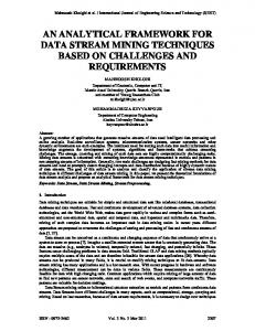
3.2. DataStreamTask After choosing a DSD class to use for data generation, the next step in the workflow is to define a DataStreamTask (DST). In stream, a DST refers to any data mining task that can be applied to data streams. We have purposefully left this ambiguous so that additional modules can be defined in the future to extend upon the DST base class. In general however, DSTs fall in two categories: data stream classification algorithms, and data stream clustering algorithms. In the current implementation of stream there are only DataStreamClusterer (DSC) classes defined, but Figure 3 shows how additional tasks can easily extend from DST as shown by the addition of the abstract class DataStreamClassifier in the diagram. It is important to note that the concept of the DST class is merely for conceptual purposes—in the actual implementation of stream there is no direct definition of DST because little is shared between the clustering and classification operations. Under the DSC class, there is a further inheritance hierarchy in which DSC_R and DSC_MOA extend the base DSC class. This is to differentiate the underlying implementation details of each class under the two separate branches. Due to the state of our implementation, the following section will mainly focus on the DSC classes that have been developed, while also providing guidance on how the same principles can be applied to other data mining tasks such as classification. The base DSC class defines several functions that are inherited by each subclass. Similar to the architecture of the DSD class, each subclass must also provide a constructor individually. get_centers(x, ...)—is a generic function that will return the centers, either the centroids or the medoids, of the micro-clusters of the DSC object if any are available. nclusters(x)—returns the number of micro-clusters in the DSC object. print(x, ...)—prints common attributes of the DSC object. Currently it prints a small

10


DataStreamTask

DataStreamClusterer

DataStreamClassifier

...

... DSC_R

DSC_tNN

DSC_MOA

...

DSC_DenStream

DSC_Clustream

DSC_CobWeb

...

Figure 3: UML diagram of the DST architecture. description of the underlying algorithm and the number of micro-clusters that have been calculated. plot(x, ..., method="pairs")—plots the centers of the micro-clusters. There are 3 available plot methods: pairs, plot, or pc. pairs is the default method that produces a matrix of scatter plots that plots the attributes against one another (this method is only available when d > 2). plot simply takes the first two attributes of the matrix and plots it as x and y on a scatter plot. Lastly, pc performs Principle Component Analysis (PCA) on the data and projects the data to a 2 dimensional plane and then plots the results. At the moment, all of our DSC classes that have been developed use MOA implementations of data stream clustering algorithms as their core and use rJava interfaces to communicate with the Java code. Currently, the only exception to this is DSC_tNN which is written entirely in R and uses some of R’s more advanced features to create mutable objects. The data stream clustering algorithms that are available in stream are StreamKM++ (Ackermann, Lammersen, M¨ artens, Raupach, Sohler, and Swierkot 2010), threshold Nearest Neighbor as seen in (Hahsler and Dunham 2010a,b), ClusTree (Kranen, Assent, Baldauf, and Seidl 2009), DenStream (Cao et al. 2006), Clustream (Aggarwal et al. 2003), and CobWeb (Fisher 1987). It is important to note that many data stream clustering algorithms consist of two parts: an online component that clusters the incoming data points into micro-clusters, and an offline component that performs a traditional clustering algorithm on the micro-clusters. Our DSC implementations only include the online segment of these algorithms. This is to allow the user to choose how they would like to manipulate the micro-clusters during the offline phase. For example, a user may want to only use a single DSC class, but may be interested in how different traditional clustering algorithms perform on the micro-clusters generated. As mentioned before, Appendix A contains all of the details concerning each implemented class.

3.3. Class Interaction Due to the abstraction in our workflow, the two step process will be similar for each combination of selected classes. Theoretically every DSD class will work flawlessly with any chosen DST class, although the results generated may not be optimal for every combination. Each subclass of the base DST also requires a set of input functions that will pull data from the DSD object and pass it to the DST object. In a classification example, these functions may be called learn() and classify() to signify the two main steps in data stream classification.


11

cluster(dsc, dsc, n)

DataStreamClusterer

DataStreamData

Results

Figure 4: Interaction between the DSD and DSC classes For our implementation of the clustering task, we use a single function called cluster() to drive the interaction. cluster(dsc, dsd, n=1000)—accepts a DSC object, a DSD object, and the number of points that will be generated by the DSD and passed to the DSC. Internally, cluster() also includes polymorphic implementations for each direct subclass of DSC, in this case, DSC_R and DSC_MOA. These internal implementations handle the different expectations by each DSC subclass: the MOA classes expect their data points to be packaged as Java Instance objects, while the R classes require no such packaging. The underlying clustering within the DSC changes during this process—no new clustering is created for each call to cluster(). Figure 4 demonstrates the interaction between a DSD object, a DSC object, and cluster(). After the clustering operation is finished, the results can be obtained from the DSC object by calling get_centers(), or they can be plotted directly to a chart by calling plot().

3.4. Extension In order to make our framework easily extendable, we have developed a set of core functions that are necessary for each component. As mentioned earlier, the actual stream implementation contains no definition for the DST concept—it is used only in the description of the design to show that all data stream mining tasks extend from the same base class. This section will outline the key functionality that needs to be available in the extension of the stream components. The core implementation of extension classes can be written in either R, Java, or C/C++, however, every class needs an R wrapper that can communicate with the rest of the framework. DSD classes need a way to either generate or retrieve data that can be used as a stream for input to DST objects. Ideally, users will be able to alter the properties in the DSD class by passing parameters in the constructor. Common properties include the number of clusters to generate, the dimensionality of the data, the distribution of the data generated, how the data evolves over time, etc. Although these properties are desirable to control, it isn’t always possible to do this in the implementation (similar to how we limit the input parameters of

12


DSD_MOA). For DSD classes, there is only a single function in addition to a constructor that is needed in order to fulfill the interface, and that function is get_points(). This function simply returns an R matrix of the data created by the DSD. It is used mainly in the cluster() function to input data into DST objects that will perform data mining operations on them. The DSC interface requires more work in that there are currently 2 abstract classes that extend directly from the abstract base class, DataStreamClusterer. Depending on which programming language is used to extend the DSC class, the new class must extend from the appropriate direct subclass of DSC. For example, all of our DSC objects that are implemented using MOA’s Java code, extend from the class DSC_MOA in addition to the base class DSC. New classes that are developed should extend the inheritance hierarchy in a similar way. If there is no concept of the subclass already included in the framework, for example, DSC_C, it is the job of the developer to create this intermediary class so that others may extend from it in the future. Note that all the extensions are from the DSC class rather than the DST class—new classes will also need to be created for other data stream tasks such as classification. For DSC subclasses, there are two functions that need be implemented in addition to the constructor. These functions are cluster() and get_centers(). The clustering function is used in conjunction with a DSD object and will feed data into the DSC object. It is responsible for updating the underlying clustering of the object (or returning a copy of the object with the updated clustering) with the data that is being streamed. cluster() should be able to handle data of any dimensionality. The get_centers() function returns a matrix that represents the centers of micro-clusters from the particular DSC object. If the underlying clustering is an object in Java, the get_centers() function should convert this to an R object before returning.

4. Examples Experimental comparison of data streams and algorithms is the main purpose of stream. In this section we give several examples in R that exhibit stream’s benchmarking capabilities. The examples become increasingly complex through the section. First, we start by giving a brief introduction to the syntax of stream by using a pair of DSC and DSD objects. The second example shows how to save stream data to disk for use in later experiments. We then give examples in how to reuse a data stream so that multiple algorithms can use the same data points, and how to use DSC classes to cluster stream data. Finally, the last example demonstrates a detailed comparison of two algorithms from start to finish by first running the online components on the same data stream, then using k-means to cluster the micro-clusters generated by each algorithm.

4.1. Creating a data stream The first step in every example is to load the package. > library("stream") In this example, we would like to focus on the merits of the DSD class to model data streams. Currently there are 4 available classes: DSD_Gaussian_Static, DSD_MOA, DSD_ReadStream,


13

and DSD_DataFrame. The syntax of creating an instance of each of the classes is consistent throughout. Below we show the creation of a DSD_Gaussian_Static object. We would like the data to be 2 dimensional, and to be generated by 3 clusters—these properties are shown as parameters during the creation. > dsd dsd DSD - Data Stream Datasource: Static R Data Stream With 3 clusters in 2 dimensions Now that we have a DSD object created we can call the get_points() function on it to generate stream data. It accepts a DSD object and n number of points and returns a numeric matrix composed of n rows and d columns. The points in this matrix are generated by different clusters defined during the creation of the DSD object. > data data

[1,] [2,] [3,] [4,] [5,] [6,] [7,] [8,] [9,] [10,] [11,] [12,] [13,] [14,] [15,] [16,] [17,] [18,] [19,] [20,] [21,]

[,1] [,2] 0.58103679 0.71299175 0.02120235 0.09662967 0.13777265 -0.01048796 0.85565828 0.37321099 0.01076491 0.03976144 0.80023353 0.51555724 0.37319813 0.73524195 0.84824710 0.37114759 0.82355266 0.51118316 0.23776072 0.09012323 0.39453182 0.65325018 0.10098767 0.08306642 0.37240061 0.64012581 0.75321682 0.53852338 0.77801012 0.37578506 0.14534009 0.14542760 0.69547988 0.52579018 0.06068131 0.02235240 0.47119824 0.74388747 -0.05211717 0.29306132 0.27865162 0.68651610

14


[22,] 0.75654364 0.65048495 [23,] 0.36029463 0.72069104 [24,] 0.08377363 -0.06119958 [25,] 0.80450365 0.43620415 attr(,"assignment") [1] 2 3 3 2 3 2 1 2 2 3 1 3 1 2 2 3 2 3 1 3 1 2 1 3 2 Additionally, by setting the parameter assignment in the get_points() function to TRUE, get_points() will also show which clusters the data points belong to. The assignment vector is shown in the code following. > attr(data, "assignment") [1] 2 3 3 2 3 2 1 2 2 3 1 3 1 2 2 3 2 3 1 3 1 2 1 3 2 n can be of any size as long as the created matrix is able to fit into memory. When data is being clustered however, get_points() is typically called for a single point at a time. This allows us both to simulate a streaming process, and to limit the amount of memory used by the created data at any given time. The data produced can then be used in any choice of application. Because the data is 2 dimensional in this case, we are able to easily plot the dimensions directly on to the x and y plane. Figure 5 shows 1000 data points from the same DSD object. In the plot there are 3 distinguishable clusters as defined in the creation of dsd. > plot(get_points(dsd, 1000)) We can also create streams with dynamic data by using the DSD_MOA class. It is important during the creation of a DSD_MOA object that values are assigned to the modelSeed and instanceSeed parameters. This ensures that new data will be produced with your experiment. Figure 6 shows the concept drift in DSD_MOA as the initial 3 clusters move around, and 2 of the clusters merge in (c). The DSD_MOA class is useful for testing how algorithms behave with dynamic data, and clusters that may merge with others over time. > dsd plot(get_points(dsd, 3000)) > plot(get_points(dsd, 3000)) > plot(get_points(dsd, 3000))

4.2. Reading and writing data streams Sometimes it is useful to be able to access the data generated by the data streams outside of the R environment. stream has support for reading and writing data streams through an R connection. Connections can be opened to a number of different sources and layouts (see the R Reference Manual for a detailed explanation (R Development Core Team 2005)). In our example, we will focus on reading from and writing to a file on disk. We start by loading the package and creating a DSD object. In our DSD object we are using data with a dimensionality of 5 to demonstrate how large streams are stored on disk.


0.6

0.8

● ● ●● ● ●● ● ● ● ● ● ● ● ●● ● ●● ●● ● ●●● ●●● ● ●● ● ● ● ● ● ● ●● ●● ● ●● ●● ● ● ● ● ●● ● ●● ● ●● ●●●● ●● ● ●● ● ● ●● ● ●●●● ● ● ●● ● ● ● ●● ● ● ●● ●● ● ●● ● ●●● ● ●● ● ● ● ● ● ●● ●● ● ● ● ● ● ● ● ● ● ● ● ● ● ●● ● ● ● ●● ● ● ● ● ● ● ● ● ● ●● ●● ● ● ● ● ● ●● ●● ●● ● ● ●● ● ● ● ● ● ● ●● ● ● ● ●● ●● ● ● ● ● ●● ●● ● ● ● ●● ● ● ● ●● ● ● ● ● ● ●● ●● ●● ● ●● ● ● ●● ● ● ● ● ●● ● ●● ● ●●●● ● ● ● ● ● ● ● ● ● ● ● ● ● ● ● ● ●● ● ●●● ●● ●● ● ● ●●● ● ●● ● ● ● ● ●● ● ●● ● ●● ● ●●● ● ●●● ● ●● ● ●●●● ●● ● ● ●● ● ● ● ● ●● ● ● ● ● ● ● ● ● ● ●● ● ●●●●●●● ●●● ●●● ● ●●● ● ●● ● ● ● ● ● ● ●●● ●● ●●●● ● ● ● ● ● ● ● ● ● ●● ● ● ● ● ● ● ● ● ● ● ● ● ●● ● ● ●●●●● ●● ●● ● ●● ● ● ●● ● ● ● ● ● ● ● ● ● ● ● ● ● ●●●● ● ● ● ●●● ● ●●● ● ● ● ● ● ● ● ● ● ● ● ●●● ● ●● ● ● ● ● ● ● ● ●●●●● ● ● ● ●● ●●● ● ●● ●● ●● ●● ●●● ●● ● ●● ● ●●● ●● ●●● ●●● ● ● ● ● ●●● ●● ● ●● ● ● ●● ● ● ● ● ●●● ● ● ● ● ●●●● ● ● ● ● ● ● ● ● ● ● ● ● ● ● ● ● ● ● ●● ●●●●●● ●● ● ● ● ● ●

0.4 0.2 −0.2

0.0

get_points(dsd, 1000)[,2]

●

15

●

●

● ●

●

●

● ●● ● ● ● ● ● ● ● ● ●● ● ● ●●● ● ● ● ● ●●●●●● ● ● ● ●● ● ●● ● ●●● ● ●●●● ● ● ● ● ● ● ● ● ● ● ● ● ● ● ● ●● ● ● ●●●● ●● ● ● ● ●● ● ● ● ● ● ● ● ● ● ● ● ●●● ● ● ● ● ● ●● ● ●● ● ● ●● ●● ●● ● ●●● ● ● ● ●● ●● ●● ● ● ● ● ● ● ● ● ● ● ● ● ● ●● ●●● ● ●● ● ●● ●● ●● ● ●●● ● ●● ●●●●● ●● ●● ● ●● ● ● ●●●● ● ●●●●●● ● ●● ●● ● ●● ● ●●●● ●●●● ● ● ● ● ● ●● ● ● ● ● ● ●●● ● ● ● ● ● ● ●● ● ● ●● ● ● ●● ● ● ● ● ● ● ● ● ● ● ● ● ● ● ● ● ●● ● ● ● ●● ● ● ●● ●● ●● ● ●● ● ● ● ● ●● ● ● ● ● ●● ●●● ● ● ● ● ● ●● ● ●● ● ● ●●●● ● ● ● ● ● ●●● ● ●●●● ● ● ●● ● ● ●● ● ● ●

−0.2

0.0

0.2

0.4

0.6

0.8

1.0


Figure 5: Plotting 100 data points from the data stream > library("stream") > dsd write_stream(dsd, "dsd_data.txt", n = 100, sep = ",", col.names = FALSE) This will create the file dsd data.txt (or overwrite it if it already exists) in the current directory and fill it with 100 data points from dsd. Now that the data is on disk, we can use a DSD_ReadStream object to open a connection to the file where it was written and treat it as a stream of data. DSD_ReadStream works in a way similar to write_stream() in that it reads a single data point at a time with the read.table() function. Again, this allows us to read from files that may be several GB in size without having to load all of the file into memory. The pairing of write_stream() and DSD_ReadStream also allows the writing and reading of .csv files. The underlying functions used in each of these interfaces can handle the row and column names that are commonly found in these types of files without changing the default parameters. These functions make it easy to use stream data created in stream in external applications—or data from external applications in stream.

● ● ●● ● ● ● ● ●● ● ● ● ● ● ● ● ● ● ● ● ● ● ● ● ● ● ● ● ● ●● ● ● ● ●● ● ● ●● ● ● ● ● ● ● ● ●● ● ● ● ● ● ● ● ● ● ● ● ● ● ● ● ● ● ● ● ● ● ● ● ● ● ● ● ● ● ● ● ● ● ● ● ● ● ● ● ● ● ● ● ● ● ● ● ● ● ● ● ● ● ● ● ● ●● ● ● ● ● ● ● ● ● ● ● ● ● ● ● ● ● ● ● ● ● ● ● ● ● ● ● ● ● ● ● ● ● ● ● ● ● ● ● ● ● ● ● ● ● ● ● ● ● ● ● ● ● ● ● ● ● ● ● ● ● ● ● ●● ● ● ● ● ● ● ● ● ● ● ● ● ● ● ● ● ● ● ● ● ● ● ● ● ● ● ● ● ● ● ● ● ● ● ● ● ● ● ● ● ● ● ● ● ● ● ● ● ● ● ● ● ● ● ● ● ● ● ● ● ● ● ● ● ● ● ● ● ● ● ● ● ●● ● ● ● ● ● ● ● ● ● ● ● ● ● ● ● ● ● ● ● ● ●●● ● ● ● ● ● ● ● ● ● ● ● ● ● ●● ● ● ● ● ● ● ● ● ● ● ● ● ● ● ● ● ● ● ● ● ● ● ●● ● ● ● ● ● ● ● ● ● ● ● ● ● ● ● ● ● ● ● ● ● ● ● ● ● ● ● ● ● ● ● ● ● ● ● ● ● ● ● ● ● ●● ● ● ● ● ●●● ● ● ●● ● ● ● ● ● ● ● ● ● ● ●● ● ● ● ● ● ● ● ● ● ● ● ● ●● ● ● ● ● ● ● ● ● ● ● ● ● ● ● ● ● ● ● ● ● ● ● ●● ● ● ● ● ● ● ● ● ● ● ● ● ● ● ● ● ● ● ● ● ● ● ● ● ● ● ● ● ● ● ● ● ● ● ● ● ● ● ● ● ● ● ● ● ● ● ● ● ● ● ● ● ● ● ● ● ● ● ● ● ● ● ● ● ● ● ● ● ● ● ● ●● ● ● ● ● ● ● ● ● ● ● ● ● ● ● ● ●● ● ● ● ● ● ● ● ● ● ● ● ● ● ● ● ● ● ● ● ● ● ● ● ● ● ● ● ● ● ● ● ● ● ● ● ● ● ● ● ● ● ● ● ● ● ● ● ● ● ● ● ● ● ● ● ● ● ● ● ● ● ● ● ● ● ● ● ● ● ● ● ● ● ● ● ● ● ● ● ● ● ● ● ● ● ● ● ● ● ● ● ● ● ● ● ● ● ● ● ● ● ● ● ● ● ● ● ● ●● ● ● ● ● ● ● ● ● ● ● ● ● ● ● ● ● ● ● ● ● ● ● ● ● ● ● ● ● ● ● ● ● ● ● ● ● ● ● ● ● ● ● ● ● ● ● ● ●● ● ● ● ● ● ● ● ● ● ● ● ● ● ● ● ● ● ● ● ● ● ● ● ● ● ● ● ● ● ● ● ● ● ● ● ●● ● ● ● ● ● ●● ● ● ● ● ● ● ● ● ● ● ● ● ● ● ● ● ● ●●● ●● ● ● ● ●● ●●● ● ●● ● ● ● ● ● ●● ● ● ● ●●● ●● ● ● ●● ● ●● ●● ● ● ●● ● ● ● ●● ●● ● ● ● ● ● ● ● ● ● ● ● ● ● ● ●● ● ● ● ● ●● ●● ● ● ● ● ● ●● ● ● ● ● ● ● ● ● ● ● ● ●● ●● ● ● ● ● ● ● ● ● ● ● ● ● ● ● ● ● ● ● ● ● ●● ● ● ●● ● ● ● ●● ● ● ● ● ● ● ● ● ● ● ● ● ● ● ● ● ● ● ● ● ● ● ● ● ● ● ● ● ● ● ● ● ● ● ● ● ● ● ● ● ● ● ● ● ● ●● ● ● ● ● ● ● ● ● ●● ● ● ● ● ● ● ● ● ● ● ● ● ● ● ● ● ● ● ● ● ● ● ● ● ● ●● ● ● ● ● ● ● ● ● ● ● ● ● ● ● ● ● ● ● ● ● ● ● ● ● ● ● ● ● ● ● ● ● ● ● ● ● ● ●●● ● ● ● ● ● ● ● ● ● ● ● ● ● ● ● ● ● ● ●● ● ● ● ● ● ● ● ● ● ● ● ● ● ● ● ● ● ● ● ● ● ● ● ● ● ●●● ● ● ● ● ●● ● ● ● ● ● ● ● ● ● ● ● ● ● ● ● ● ● ● ● ● ● ● ● ● ● ● ● ● ● ● ● ● ● ● ● ● ● ● ● ● ● ● ● ● ● ● ● ● ● ● ● ●● ● ● ● ● ● ● ● ● ● ● ● ● ● ● ● ● ● ● ● ● ● ● ● ● ● ● ● ● ● ● ● ● ● ● ● ● ● ● ● ● ● ● ● ● ● ● ● ● ● ● ● ● ● ● ● ● ● ● ● ● ● ● ● ● ● ● ● ● ● ● ● ● ● ● ● ● ● ● ● ● ● ● ● ● ● ● ● ● ● ● ● ● ● ● ● ● ● ● ● ● ●● ● ● ● ● ● ● ● ● ● ● ●● ● ● ●● ● ●● ● ● ● ● ● ● ● ● ● ● ● ● ● ● ●● ● ● ● ● ● ● ● ● ● ● ● ● ● ● ● ● ●● ● ● ● ● ● ● ●● ● ● ● ● ● ● ● ● ● ●● ● ● ● ● ●● ● ● ● ● ●

●

●

0.0

0.2

0.4

0.6

0.8

1.0


1.0

● ●

0.6 0.4 0.2 0.0


0.8

● ● ● ●

● ●

●● ● ●

●● ●● ● ● ● ● ●● ● ● ● ●●

0.0

0.8 0.6 0.4 0.2 0.0

● ●●

●

●

0.2

0.4

(b)

●● ●

● ●● ●● ●

● ●● ● ●

●

● ● ●

● ●● ● ● ●● ● ● ● ● ● ● ● ● ● ● ● ● ● ● ● ● ● ● ●● ● ●● ● ● ● ● ● ●● ● ● ● ● ● ● ● ● ● ● ● ● ● ● ● ● ● ● ● ● ●● ● ● ● ● ● ● ●● ● ● ● ● ● ● ● ● ● ● ● ● ● ● ● ● ● ● ● ● ● ● ● ● ● ● ● ● ● ● ● ● ● ● ● ● ● ● ● ● ● ● ● ● ● ● ● ● ● ● ● ● ● ● ● ● ● ● ● ● ● ● ● ● ● ● ● ● ● ● ● ● ● ● ● ● ● ● ● ● ● ● ● ● ● ● ● ● ● ● ● ● ● ● ● ● ● ● ● ●● ● ● ● ● ● ● ● ● ● ● ● ● ● ● ● ● ● ● ● ● ● ● ● ● ● ● ● ●● ● ● ● ● ● ● ● ● ● ● ● ● ● ● ● ● ● ● ● ● ● ● ● ●● ● ● ● ● ● ● ● ● ● ● ● ● ● ● ● ● ● ● ● ●● ● ● ● ● ● ● ● ● ● ● ● ● ● ● ● ● ● ● ● ● ● ● ● ● ● ● ● ● ● ● ● ● ● ● ● ● ● ● ● ● ● ● ● ● ● ● ● ● ● ● ● ● ● ● ● ● ● ● ● ● ● ● ● ● ● ● ● ● ● ● ● ● ● ● ● ● ● ● ● ● ● ● ● ● ● ● ● ● ●● ● ● ● ● ● ● ● ● ● ● ● ● ● ● ● ● ● ● ● ● ● ● ● ● ● ● ● ●● ● ● ● ● ● ● ● ● ● ● ● ● ● ● ● ● ● ● ● ●● ● ● ● ● ● ● ● ● ● ● ● ● ● ●● ● ● ● ● ● ● ● ● ● ● ● ● ● ● ● ● ● ● ● ● ● ● ● ● ● ● ● ● ● ● ● ● ● ● ● ● ● ● ● ● ● ● ● ● ● ● ● ● ● ● ● ● ● ●● ● ● ● ●● ● ● ● ● ● ● ●● ●● ● ● ● ● ● ●● ● ● ● ● ● ● ● ● ● ● ● ● ● ● ● ● ● ●● ●● ● ● ● ● ● ● ● ● ● ● ● ● ●● ● ● ● ● ●● ● ● ● ● ● ● ● ●● ● ● ● ● ● ● ● ● ● ● ● ● ● ● ● ● ● ● ● ● ● ● ● ● ● ● ● ● ● ● ● ● ●● ● ● ●● ● ● ● ● ● ● ● ● ●● ●● ● ● ● ● ●● ●● ● ●● ●● ● ● ● ● ● ● ● ● ● ● ● ● ● ● ● ● ● ● ● ● ● ● ● ● ● ●● ● ● ● ● ● ● ● ● ● ● ● ● ● ● ● ● ● ● ● ● ● ● ● ● ● ● ● ● ● ● ● ● ● ● ● ● ● ● ● ● ● ● ● ● ● ● ● ● ● ● ● ● ● ● ● ● ● ● ● ● ● ● ● ● ● ● ● ● ● ● ● ● ● ● ● ● ● ● ● ● ● ● ● ● ● ● ● ● ● ●● ● ● ● ● ● ● ● ● ● ● ● ● ● ● ● ● ● ● ● ● ● ● ● ● ● ● ● ● ● ● ● ● ● ● ● ● ● ● ● ● ● ● ● ● ● ● ● ● ● ● ● ● ● ● ● ● ● ● ● ● ● ● ● ● ● ● ● ● ● ● ● ● ● ● ● ● ● ● ● ● ● ● ● ● ● ● ● ● ● ● ● ● ● ● ● ● ● ● ● ● ● ● ● ● ● ● ● ● ● ● ● ● ● ● ● ● ● ● ● ● ● ● ● ● ● ● ● ● ● ● ● ● ● ● ● ● ● ● ● ● ●● ● ● ● ● ● ● ● ● ●● ● ● ● ● ● ● ● ● ● ● ● ● ● ● ● ● ● ● ● ● ● ● ● ● ● ● ● ● ● ● ● ● ● ● ● ● ●● ● ● ● ● ● ● ● ● ●● ● ● ● ● ● ● ● ● ● ● ● ● ● ●● ● ● ● ● ● ● ● ● ● ● ● ● ● ●● ● ●● ●●

0.0

0.2

0.4

0.6

0.6


(a)

● ●

●● ● ●● ● ● ● ● ● ● ● ● ● ● ●● ● ● ● ●● ● ● ● ● ● ● ● ● ● ● ● ● ● ● ● ● ● ● ● ● ● ●● ● ● ● ●● ● ● ●● ● ● ● ● ● ● ● ● ●●● ● ● ● ● ● ● ●● ●● ● ● ● ● ● ● ● ● ● ● ● ● ● ● ● ● ● ● ● ● ● ● ● ● ● ● ● ● ● ● ● ● ● ● ● ● ● ● ● ● ● ● ● ●● ● ● ● ● ●●●● ● ● ●● ● ● ● ● ● ● ● ● ● ● ● ● ● ● ● ● ● ● ● ● ● ● ● ● ●● ● ● ● ● ● ● ● ● ● ● ● ● ● ● ● ● ● ● ● ● ● ● ● ● ● ● ● ● ● ● ● ● ●● ● ● ● ● ● ● ● ● ● ● ● ● ● ● ● ● ● ● ● ● ● ● ● ● ● ● ● ● ● ● ● ● ● ● ● ● ● ●● ● ● ● ● ● ● ● ● ● ● ● ● ● ● ● ● ● ● ● ● ● ● ● ● ● ● ●● ● ● ● ● ● ● ● ● ● ● ● ● ● ● ● ● ● ● ● ● ● ● ● ● ● ● ● ● ● ●● ● ● ● ● ● ● ● ● ● ● ● ● ● ● ● ● ● ● ● ● ● ● ● ● ● ● ● ● ● ● ● ● ● ● ● ● ● ● ● ● ● ● ●● ● ● ● ● ● ● ● ● ● ● ● ● ● ● ● ● ●● ● ● ● ● ● ●● ● ● ● ● ● ● ● ● ● ● ● ● ● ● ● ● ● ● ● ● ● ● ● ●● ● ● ● ● ● ● ● ● ● ● ● ● ● ● ● ● ● ● ● ● ● ● ● ● ● ● ● ● ● ● ● ● ● ● ● ● ● ● ● ● ● ● ● ● ● ● ● ● ● ● ● ● ● ● ● ● ● ● ● ● ● ● ● ● ● ● ● ● ● ● ● ● ● ● ● ● ● ● ● ● ● ● ● ● ● ● ● ● ● ● ● ● ● ● ● ● ● ● ● ● ● ● ● ● ● ● ● ● ● ● ● ● ● ● ● ●● ● ● ● ● ● ● ● ● ● ● ● ● ● ● ● ● ●● ● ● ● ● ● ● ● ● ● ● ● ● ● ● ● ● ● ● ● ● ● ● ● ● ● ● ● ● ● ● ● ● ● ● ●●● ● ● ● ● ● ● ● ● ● ● ● ● ● ● ● ● ● ● ● ● ● ● ● ● ● ● ●● ●● ● ● ● ● ● ● ● ● ● ● ● ● ● ● ● ● ● ● ● ● ● ● ● ● ● ● ● ● ● ● ● ● ● ● ● ● ● ● ● ● ● ● ● ● ● ● ● ● ● ● ● ● ● ● ● ● ● ● ●● ● ● ● ● ● ● ● ● ● ● ● ● ● ● ● ● ● ● ● ● ● ● ● ● ● ● ● ● ● ● ● ● ● ● ● ● ● ● ● ● ● ● ● ● ● ● ● ● ●● ● ● ● ● ● ● ● ● ●● ● ● ● ● ● ● ● ● ● ● ●● ● ● ● ●● ● ● ● ●● ● ● ● ●● ● ● ● ● ● ● ● ● ● ● ● ● ●● ● ● ● ● ● ● ● ●● ● ● ● ● ● ● ● ● ● ● ● ● ● ● ● ● ● ● ● ● ● ● ● ● ● ● ● ● ●● ● ● ● ● ● ● ● ● ●● ●● ● ● ● ● ● ● ● ● ● ● ● ● ● ● ● ● ● ●●● ● ●● ● ● ● ● ● ● ● ● ● ● ● ● ● ● ● ● ● ● ● ● ● ● ● ● ● ● ● ● ● ● ● ● ● ● ● ● ● ●● ● ● ● ● ● ● ● ● ● ● ● ● ● ● ● ● ● ● ●● ● ● ● ● ● ● ● ● ● ● ● ● ● ● ● ● ● ● ● ● ● ● ● ● ● ● ● ● ● ● ● ● ● ● ● ● ● ● ● ● ● ● ● ● ●● ● ● ● ● ● ● ● ●● ● ● ● ● ● ● ● ● ● ● ● ● ● ● ● ● ● ● ● ● ● ● ● ● ● ● ● ● ● ● ● ● ● ● ● ● ● ● ● ● ●● ● ● ● ● ● ● ● ● ● ● ● ● ● ● ● ● ● ● ● ● ● ● ● ● ● ● ● ● ● ● ● ● ● ● ● ● ● ● ● ● ● ● ● ● ● ● ● ● ● ● ● ● ● ● ● ● ● ● ● ● ● ● ● ● ● ● ● ● ● ● ● ● ● ● ● ● ● ● ● ● ● ● ● ● ● ● ● ● ● ● ● ● ● ● ● ● ● ● ● ● ● ● ● ● ● ● ● ● ●● ● ● ● ● ● ● ● ● ● ● ● ● ● ● ● ● ● ● ● ●● ● ● ● ● ● ● ● ● ● ● ● ● ● ● ● ● ● ● ● ● ● ● ● ● ● ● ● ● ● ● ● ● ● ● ● ● ● ● ● ● ● ● ● ● ● ● ● ● ● ● ● ● ● ● ● ● ● ● ● ● ● ● ● ● ● ● ● ● ● ●● ● ● ● ● ● ● ● ● ● ● ● ●

●

● ●


0.8 0.6 0.4 0.0

0.2


●● ●● ● ● ●

1.0


1.0

16

0.8

1.0


(c) Figure 6: The concept drift of DSD MOA

0.8

1.0


17

> dsd2 > > >

library("stream") dsd replayer

18


DSD - Data Stream Datasource: Data Frame/Matrix Wrapper Stream With 3 clusters in 2 dimensions Contains 100 data points, currently at position 101 loop is FALSE > reset_stream(replayer) > replayer DSD - Data Stream Datasource: Data Frame/Matrix Wrapper Stream With 3 clusters in 2 dimensions Contains 100 data points, currently at position 1 loop is FALSE

4.4. Clustering a data stream This example outlines how to cluster data using DSC objects. Again, start by loading stream. > library("stream") Next, create the DSC and DSD objects. In this example we use the DSC_DenStream class with its default parameters, and DSD_Gaussian_Static with 2 dimensionality data generated from 3 clusters. We also created a DSD_DataFrame so that we can use the same data used in the clustering operation to plot the micro-clusters against. Notice that the noise parameter is set to 0.05, the enabling of this parameter causes 5% of the data points generated by the DSD to be noise. > dsc d head(d)

[1,] [2,] [3,] [4,] [5,] [6,]

[,1] 0.7990691 0.1045328 0.1409029 0.8889469 0.1278920 0.8165545

[,2] 0.44333951 0.02173426 0.03561777 0.25343851 0.02629838 0.56860559

> dsd dsd DSD - Data Stream Datasource: Data Frame/Matrix Wrapper Stream With 3 clusters in 2 dimensions Contains 3000 data points, currently at position 1 loop is FALSE Now, the objects need to interact with one another through the cluster() function. The clustering operation will implicitly alter dsc so no reassignment is necessary. By default, DSC_DenStream is initialized with 1000 points, meaning that no new micro-clusters are created until this threshold has been breached, which is why we cluster 3000 new data points.

1.0


●● ● ● ● ● ● ● ● ● ● ● ● ● ● ● ● ●● ● ● ● ● ● ● ●● ● ● ●●●●● ●● ● ● ● ● ● ● ● ●●● ● ● ● ● ● ● ● ● ● ● ● ● ● ● ● ●● ●●● ●● ●● ● ●● ●● ●●● ● ● ● ● ● ● ● ● ●●● ●●● ● ● ● ● ● ●● ● ● ● ● ● ● ● ● ●● ● ● ● ● ● ● ● ● ● ● ● ● ● ● ●● ● ● ● ● ● ● ●● ● ● ● ●● ● ● ● ●● ● ● ● ● ●● ● ● ● ● ● ● ● ● ● ● ● ● ● ● ● ● ● ● ● ● ● ●● ● ●● ● ● ● ● ● ● ● ● ● ● ● ● ● ● ● ● ● ● ● ● ● ● ● ● ●● ● ● ● ● ● ●● ● ● ● ● ● ● ● ● ● ● ● ● ● ● ● ● ● ● ●● ●● ● ● ● ● ● ● ● ● ● ● ● ● ● ● ● ● ● ●●● ● ● ●● ● ● ● ● ●●● ● ● ● ● ● ● ● ● ● ● ● ● ● ● ● ● ● ● ●● ● ● ● ● ●● ● ● ● ● ● ● ● ● ● ● ● ● ● ● ● ● ● ● ● ● ● ● ● ● ● ● ●●●● ● ● ● ● ● ● ● ● ● ● ● ● ● ● ● ● ● ● ● ● ● ● ● ● ● ● ● ● ● ● ● ● ● ● ● ● ● ● ● ● ● ● ● ● ● ● ● ● ● ● ● ● ● ● ● ● ● ● ● ● ● ● ● ● ● ● ● ● ● ● ● ● ● ●● ●● ● ● ● ● ● ●● ● ●● ●●●● ● ● ● ● ● ● ● ● ● ● ● ● ● ● ● ● ● ● ● ● ● ● ● ● ● ●● ● ● ●● ● ● ● ●● ● ● ● ● ● ●● ● ● ● ● ● ● ● ● ● ● ● ● ● ● ● ● ● ● ● ● ● ● ● ● ● ● ●●●● ● ● ● ● ● ● ● ● ● ● ● ● ● ● ● ● ● ● ● ● ●● ● ● ● ● ● ●● ● ● ● ● ● ● ● ● ● ● ● ●● ●●●● ● ● ● ● ● ● ● ● ● ●● ●●● ● ● ● ● ●● ● ● ● ● ● ● ● ● ● ● ● ● ● ● ● ● ● ● ● ●● ● ●● ● ● ● ● ● ● ● ● ● ● ● ●● ● ● ● ● ● ● ● ●●● ● ● ● ● ● ● ● ●● ● ● ● ●● ● ● ● ●● ●● ● ● ● ● ● ● ● ●● ● ● ● ● ●● ● ● ● ● ● ● ● ●● ● ● ● ● ● ● ● ●●● ● ● ● ● ● ● ● ● ● ●● ● ● ●● ● ● ● ● ●● ● ● ●● ● ● ● ● ●●●● ● ●● ● ● ● ● ● ● ● ● ● ● ●● ● ● ● ● ● ● ● ● ● ● ● ● ● ● ●● ● ● ● ● ● ● ● ●● ● ● ● ● ● ● ● ●● ●● ● ● ● ● ● ● ● ● ● ● ● ●● ● ● ● ●●● ● ●● ● ● ● ● ● ● ● ● ● ● ●●●● ● ● ● ● ● ● ● ●●● ● ● ● ●●●●● ● ● ● ● ● ● ●● ● ● ● ● ●● ● ● ● ● ●● ● ● ● ● ●● ● ● ● ● ● ● ●●●● ● ● ● ● ● ● ● ●● ● ● ● ● ● ● ● ● ● ●● ● ● ●●●● ● ● ● ● ● ●●● ● ● ● ● ● ● ● ● ● ● ● ● ● ● ● ● ● ● ● ● ●● ● ● ●● ● ● ● ● ● ● ● ●●● ● ● ● ● ● ● ●● ● ● ● ● ● ● ● ● ● ●● ● ● ● ● ● ● ● ● ● ●● ● ● ● ● ● ● ● ● ● ● ● ● ● ● ● ● ● ● ● ● ● ● ● ● ● ● ● ● ● ● ● ● ● ● ● ● ● ● ● ● ● ● ● ● ● ● ● ● ● ● ●● ● ● ●● ●● ● ● ● ● ● ● ● ● ● ●● ● ● ●● ● ● ● ● ● ● ● ● ● ● ● ● ● ● ● ● ● ● ● ● ● ● ● ● ● ● ● ● ● ●● ● ● ● ● ● ● ● ● ● ● ● ● ● ● ● ● ● ● ● ● ● ● ● ● ● ● ● ● ● ● ●● ● ●● ● ● ● ● ● ● ● ● ● ● ● ● ● ● ● ● ● ● ● ● ● ● ●● ● ● ●●●● ● ●●●● ● ● ● ● ● ● ● ● ● ● ● ● ● ● ● ● ●● ● ● ● ● ● ● ● ● ● ●● ● ● ● ● ● ● ● ● ● ● ● ● ● ● ● ● ● ● ● ● ● ● ● ●● ● ● ● ● ● ● ● ● ● ● ● ● ● ● ● ● ● ● ●●● ● ● ● ● ● ● ● ● ● ● ● ● ● ● ● ● ● ● ● ● ● ● ● ● ● ● ●●●●● ● ● ● ●●● ● ● ●●● ● ● ● ● ● ● ● ● ● ● ● ● ● ● ● ● ● ● ● ● ● ● ● ● ● ● ● ● ● ● ● ● ● ● ● ● ●● ●● ● ● ● ●● ● ● ● ● ●● ● ● ● ● ● ●● ● ● ● ● ● ● ● ● ● ● ● ● ● ● ● ● ●● ●●● ●● ● ● ●● ● ●● ●● ● ● ● ● ● ● ● ● ● ● ●● ●● ● ● ● ●● ● ● ●● ● ●● ●● ●●●● ● ●● ● ●●● ● ● ● ● ●● ● ● ● ● ● ● ● ● ●● ● ● ●●● ●●● ● ●● ●● ● ●●● ●● ● ● ● ●● ● ● ● ● ●●●●● ● ● ● ● ●● ●● ● ● ●●● ● ● ● ● ● ● ● ● ● ● ● ● ● ● ● ● ● ● ● ● ● ● ● ●● ● ● ● ● ●● ●● ● ●● ● ●● ● ●● ● ● ● ● ●● ●●●● ● ● ● ● ● ●● ● ● ● ●● ● ●● ● ● ●●● ● ●● ● ● ● ●●● ● ●● ● ●● ● ● ● ● ● ● ● ●● ● ● ● ● ●●● ● ● ●● ● ● ● ● ● ● ● ● ● ● ● ● ● ● ●● ● ● ●● ● ● ● ● ● ● ●● ● ●● ● ● ● ● ● ● ● ● ● ● ● ● ● ●●● ● ● ●● ● ● ● ● ● ● ● ● ● ● ● ● ● ● ● ● ● ● ● ● ● ● ● ● ● ● ● ● ●● ● ● ● ● ● ● ● ● ● ● ● ● ● ● ●● ● ● ● ● ● ● ● ● ● ●● ● ● ● ● ● ● ● ● ● ● ● ● ● ● ● ● ● ● ● ● ● ● ● ● ● ● ● ● ● ● ● ● ● ● ● ● ● ● ● ● ● ● ● ●●● ●● ● ● ●● ● ● ● ●● ●● ● ● ● ● ● ● ● ● ● ● ● ●● ●●● ● ● ● ● ● ● ● ● ● ●●● ● ● ● ● ● ● ● ● ● ● ● ● ● ● ●● ●●● ● ● ● ● ● ● ● ● ● ● ● ● ● ● ● ● ●● ● ● ● ● ●● ● ●● ● ● ●● ● ● ● ● ● ●● ●● ● ● ●● ● ● ● ● ● ● ● ● ●● ● ● ● ● ● ● ● ● ● ● ● ● ● ● ● ● ● ● ● ● ● ● ● ● ● ●●● ● ● ●● ● ● ● ● ● ● ●● ●● ● ● ● ● ● ● ● ● ● ● ● ● ● ● ● ●● ● ● ● ● ● ●● ● ● ●● ● ● ● ●●● ● ● ● ● ● ● ● ● ● ● ● ● ● ● ●● ● ● ● ● ● ● ● ●● ● ● ● ● ●● ● ● ● ● ● ● ● ● ● ● ● ●● ● ● ● ● ● ●● ● ● ● ● ● ● ● ● ●● ● ● ● ● ● ● ● ● ●● ● ●● ● ● ● ● ● ● ● ● ● ● ● ● ●● ● ● ● ●● ● ● ● ●● ● ● ●● ● ● ● ● ● ● ●●● ● ●● ● ● ● ● ● ●● ●● ● ● ● ● ● ● ● ● ● ● ● ● ● ● ● ● ● ● ● ● ● ● ● ● ●● ● ● ● ●●● ●● ●●● ●● ●●● ● ●● ● ● ●● ● ●●● ● ●● ●● ● ● ●● ●● ● ●● ●● ●● ●● ●●●●● ● ● ●●●●● ● ●● ● ● ● ●● ●●● ● ● ●● ● ● ●● ● ●● ● ●● ●● ●● ● ● ● ●● ● ● ● ● ●●

−0.2

0.0

0.2

0.4

0.6

0.8

●

d[,2]

19

−0.2

0.0

●

●

0.2

0.4

0.6

0.8

1.0

d[,1]

Figure 7: Plotting the micro-clusters on top of data points > cluster(dsc, dsd, 3000) After clustering the data, we are ready to view the results. > plot(d, col = "grey") > points(get_centers(dsc), col = "red", pch = 3) Figure 7 is the result of the calls to plot() and points(). It shows the micro-clusters as red crosses on top of grey data points. It is often helpful to visualize the results of the clustering operation during the comparison of algorithms.

4.5. Full experimental comparison This example shows the stream framework being used from start to finish. It encompasses the creation of data streams, data clusterers, the online clustering of data points as micro-clusters, and then the comparison of the offline clustering of 2 data stream clustering algorithms by applying the k-means algorithm. As such, less detail will be given in the topics already covered in the previous examples and more detail will be given on the comparison of the 2 data stream clustering algorithms. Setting up the experiment: > library("stream") > d head(d)

[1,]

[,1] [,2] 0.73814935 0.59948062

20


[2,] -0.02538873 0.12382056 [3,] 0.14360917 0.03777090 [4,] 0.78384927 0.54617575 [5,] 0.11410208 0.24529526 [6,] 0.57562751 0.63880642 > dsd dsd DSD - Data Stream Datasource: Data Frame/Matrix Wrapper Stream With 3 clusters in 2 dimensions Contains 10000 data points, currently at position 1 loop is FALSE > dsc1 dsc2 > > >

cluster(dsc1, dsd, 10000) reset_stream(dsd) cluster(dsc2, dsd, 10000) dsc1

DSC - Data Stream Clusterer: DenStream Number of clusters: 145 > dsc2 DSC - Data Stream Clusterer: Clustream Number of clusters: 100 Now we plot the data and the 2 sets of micro-clusters generated. > plot(d, xlab = "x", ylab = "y", col = "grey", pch = 4, cex = 0.5) > points(get_centers(dsc2), col = "blue", cex = 2, lwd = 2) > plot(d, xlab = "x", ylab = "y", col = "grey", pch = 4, cex = 0.5) > points(get_centers(dsc1), col = "red", cex = 2, lwd = 2) The code above creates a DSD_DataFrame object from a DSD_Gaussian_Static object so that we can replay the same stream data for both DSC objects. We then use the DSD_DataFrame to feed the exact data stream into 2 different algorithms, DenStream and Clustream, during the cluster() operation. Note that after each call to cluster(), we also have to call reset_stream() to reset the DSD_DataFrame back to its original position. After the clustering operations, we plot the calculated micro-clusters and the original data. Figure 8 shows the 2 sets of micro-clusters, in red and blue, over the original data which is in

21

1.0 0.8

0.8

1.0


0.6 0.4 −0.2

0.0

0.2

●●● ● ● ●●● ● ●● ● ●● ●●●● ● ●● ●● ● ● ●

−0.2

0.0

0.2

●

y

y

0.4

0.6

● ●● ● ● ● ●● ● ● ●● ●● ● ● ● ● ● ●● ● ● ●● ● ● ● ● ● ●● ● ● ● ● ●● ●● ●● ● ● ● ●● ● ● ● ● ● ●● ● ●● ● ● ●● ● ●● ● ● ●● ● ● ● ● ● ● ● ● ●● ● ●● ● ● ● ●● ● ● ●● ●● ● ● ● ● ●●●● ●● ●● ● ●●

−0.2

0.0

0.2

0.4

0.6

0.8

1.0

● ● ● ● ● ● ●● ● ● ● ● ● ● ●●● ●● ● ● ● ●● ●● ● ● ● ● ●●●● ● ● ● ● ● ● ●● ● ● ● ●●● ● ●● ● ● ● ●●● ● ● ● ● ● ● ● ● ●● ● ● ● ● ● ●● ● ● ● ● ● ●●● ● ● ● ● ●● ● ●● ● ●●●● ● ● ●●

−0.2

0.0

0.2

0.4

x

x

(a)

(b)

0.6

0.8

1.0

Figure 8: Plotting 2 sets of different micro-clusters against the generated data grey. We have plotted the micro-clusters as circles to more closely reflect their nature, however, the circles are merely a representation and the radii haven’t been calculated specifically for each micro-cluster. The plot makes it easy to point out differences in the two algorithms. The DenStream micro-clusters, in red, stay true to the nature of the algorithm in that they congregate where there is a large number of data points, or in other words, dense areas. Clustream on the other hand, in blue, is more evenly spread, and the micro-clusters are relatively separated, covering most of the area that the generated data fills. > plot(d, xlab = "x", ylab = "y", pch = 4, cex = 0.5, col = "grey") > points(kmeans(get_centers(dsc1), centers = 3, nstart = 5)$centers, + col = "red", cex = 14, lwd = 2) > plot(d, xlab = "x", ylab = "y", pch = 4, cex = 0.5, col = "grey") > points(kmeans(get_centers(dsc2), centers = 3, nstart = 5)$centers, + col = "blue", cex = 14, lwd = 2) We can then take this a step further. Figure 9 shows a new plot—in this case, we are plotting the calculated macro-clusters of each algorithm as a result of a k-means operation. We use the term “macro” here to differentiate the k-means clusters from the micro-clusters generated by the stream clustering algorithms. Again, the DenStream clusters are shown in red, and the Clustream clusters are shown in blue. We have enlarged the circle representations for the k-means clusters to better show the area they cover. This last operation is an example of how we use the same offline component for two different algorithms, and the differences that it produces. R contains an assortment of traditional clustering algorithms that are available through the installation of various packages. It is up to the user to decide which clustering algorithm they would like to use as the offline component. Most stream clustering algorithms are developed with a certain offline algorithm in mind, but it is interesting to see the different combinations of algorithms and the results they produce.

0.8 0.6 0.4 y 0.2 0.0 −0.2

−0.2

0.0

0.2

y

0.4

0.6

0.8

1.0


1.0

22

−0.2

0.0

0.2

0.4

0.6

0.8

1.0

−0.2

0.0

0.2

0.4

x

x

(a)

(b)

0.6

0.8

1.0

Figure 9: Plotting the results of a k-means operation on each stream clustering algorithm

There are several external packages that are required to use the stream package. These include the proxy package, written by Meyer and Buchta (2010), the MASS package by Venables and Ripley (2002), and clusterGeneration by Qiu and Joe. (2009). To facilitate the communication between R and Java, we used the rJava package by Urbanek (2010). This allows us to make method calls directly to the JRI from within the R environment.

5. Conclusion and Future Work stream is a data stream modeling framework in R that has both a variety of data stream generation tools as well as a component for performing data stream mining tasks. The flexibility offered by our framework allows the user to create a multitude of easily reproducible experiments to compare the performance of these tasks. Data streams can be created with specific properties that may be difficult to simulate in real-world situations. Furthermore, the infrastructure that we have built can be extended upon in multiple directions. We have abstracted each component to only require a small set of functions that are defined in each base class. Writing the framework in R means that developers have the ability to design components either directly in R, or design components in Java or C/C++, and then write an R wrapper to use the high level code. Upon completion, stream will be available from The Comprehensive R Archive Network (CRAN) website for download (for Statistical Computing 2010). In the future, we plan on adding additional functionality to stream. Currently we only have implementations for clustering tasks; we would like to develop a classification module that also extends from the base DST class. Additionally, there are plans to develop an evaluation module that accompanies each DST class to provide immediate feedback on their performance. Finally, for each of the DST classes developed, we would like to include all of the available algorithms, both the latest innovations and the original algorithms that shaped the research for the respective area.


23

References Ackermann MR, Lammersen C, M¨artens M, Raupach C, Sohler C, Swierkot K (2010). “StreamKM++: A Clustering Algorithm for Data Streams.” In “Proceedings of the 12th Workshop on Algorithm Engineering and Experiments (ALENEX ’10),” pp. 173–187. Society for Industrial and Applied Mathematics. Aggarwal C (ed.) (2007). Data Streams – Models and Algorithms. Springer. Aggarwal C (2009). “A Framework for Clustering Massive-Domain Data Streams.” In “Proceedings of the 2009 IEEE International Conference on Data Engineering,” pp. 102–113. IEEE Computer Society, Washington, DC, USA. ISBN 978-0-7695-3545-6. Aggarwal CC, Han J, Wang J, Yu PS (2003). “A framework for clustering evolving data streams.” In “Proceedings of the 29th international conference on Very large data bases Volume 29,” VLDB ’2003, pp. 81–92. VLDB Endowment. ISBN 0-12-722442-4. Analytics R (2010). REvolution R. URL http://www.revolutionanalytics.com/. Bifet A, Holmes G, Kirkby R, Pfahringer B (2010). “MOA: Massive Online Analysis.” J. Mach. Learn. Res., 99, 1601–1604. ISSN 1532-4435. Cao F, Ester M, Qian W, Zhou A (2006). “Density-based clustering over an evolving data stream with noise.” In “In 2006 SIAM Conference on Data Mining,” pp. 328–339. Dunham MH (2002). Data Mining: Introductory and Advanced Topics. Prentice Hall PTR, Upper Saddle River, NJ, USA. ISBN 0130888923. Fisher DH (1987). “Knowledge Acquisition Via Incremental Conceptual Clustering.” Mach. Learn., 2, 139–172. ISSN 0885-6125. for Statistical Computing RF (2010). The Comprehensive R Archive Network. URL http: //cran.r-project.org/. Fowler M (2003). UML Distilled: A Brief Guide to the Standard Object Modeling Language. Addison-Wesley Longman Publishing Co., Inc., Boston, MA, USA, 3 edition. ISBN 0321193687. Guha S, Meyerson A, Mishra N, Motwani R, O’Callaghan L (2003). “Clustering Data Streams: Theory and Practice.” IEEE Transactions on Knowledge and Data Engineering, 15, 515– 528. ISSN 1041-4347. Hahsler M, Dunham MH (2010a). rEMM: Extensible Markov Model for Data Stream Clustering in R. R package version 1.0-0., URL http://CRAN.R-project.org/. Hahsler M, Dunham MH (2010b). “rEMM: Extensible Markov Model for Data Stream Clustering in R.” Journal of Statistical Software, 35(5), 1–31. URL http://www.jstatsoft. org/v35/i05/. Hahsler M, Dunham MH (2011). “Temporal Structure Learning for Clustering Massive Data Streams in Real-Time.” In “SIAM Conference on Data Mining (SDM11),” SIAM. Accepted for presentation.

24


Hall M, Frank E, Holmes G, Pfahringer B, Reutemann P, Witten IH (2009). “The WEKA data mining software: an update.” SIGKDD Explor. Newsl., 11, 10–18. ISSN 1931-0145. Kranen P, Assent I, Baldauf C, Seidl T (2009). “Self-Adaptive Anytime Stream Clustering.” In “Proceedings of the 2009 Ninth IEEE International Conference on Data Mining,” ICDM ’09, pp. 249–258. IEEE Computer Society, Washington, DC, USA. ISBN 978-0-7695-3895-2. Manning CD, Raghavan P, Schtze H (2008). Introduction to Information Retrieval. Cambridge University Press, New York, NY, USA. ISBN 0521865719, 9780521865715. Masud MM, Chen Q, Khan L, Aggarwal CC, Gao J, Han J, Thuraisingham BM (2010). “Addressing Concept-Evolution in Concept-Drifting Data Streams.” In “ICDM’10,” pp. 929–934. Meyer D, Buchta C (2010). proxy: Distance and Similarity Measures. R package version 0.4-6, URL http://CRAN.R-project.org/package=proxy. Qiu W, Joe H (2009). clusterGeneration: random cluster generation (with specified degree of separation). R package version 1.2.7. R Development Core Team (2005). R: A language and environment for statistical computing. R Foundation for Statistical Computing, Vienna, Austria. ISBN 3-900051-07-0, URL http: //www.r-project.org/. Tan PN, Steinbach M, Kumar V (2006). Introduction to Data Mining. Pearson Education. Urbanek S (2010). rJava: Low-level R to Java interface. R package version 0.8-8, URL http://CRAN.R-project.org/package=rJava. Venables WN, Ripley BD (2002). Modern Applied Statistics with S. Springer, New York, fourth edition. ISBN 0-387-95457-0, URL http://www.stats.ox.ac.uk/pub/MASS4. Wan L, Ng WK, Dang XH, Yu PS, Zhang K (2009). “Density-based clustering of data streams at multiple resolutions.” ACM Trans. Knowl. Discov. Data, 3, 14:1–14:28. ISSN 1556-4681.

Package ‘stream’ April 18, 2011 Version 0.0 Date 2010-09-29 Title Infrastructure for Data Streams Author John Forrest, Michael Hahsler Maintainer John Forrest Description A framework for data stream modelling and associated data mining tasks such as clustering and classification. Depends R (>= 2.10.0), clusterGeneration, proxy, methods Imports rJava (>= 0.6-3), MASS SystemRequirements Java (>= 5.0) License GPL-2

R topics documented: cluster . . . . . . . . . DSClusterer . . . . . . DSC_Clustream . . . . DSC_ClusTree . . . . DSC_CobWeb . . . . . DSC_DenStream . . . DSC_MOA . . . . . . DSC_StreamKM . . . DSC_tNN . . . . . . . DSData . . . . . . . . DSD_DataFrame . . . DSD_Gaussian_Static . DSD_MOA . . . . . . DSD_ReadStream . . . get_centers . . . . . . get_points . . . . . . . nclusters . . . . . . . . reset_stream . . . . . . write_stream . . . . .

. . . . . . . . . . . . . . . . . . .

. . . . . . . . . . . . . . . . . . .

. . . . . . . . . . . . . . . . . . .

. . . . . . . . . . . . . . . . . . .

. . . . . . . . . . . . . . . . . . .

. . . . . . . . . . . . . . . . . . .

. . . . . . . . . . . . . . . . . . .

. . . . . . . . . . . . . . . . . . .

. . . . . . . . . . . . . . . . . . .

. . . . . . . . . . . . . . . . . . .

Index

. . . . . . . . . . . . . . . . . . .

. . . . . . . . . . . . . . . . . . .

. . . . . . . . . . . . . . . . . . .

. . . . . . . . . . . . . . . . . . .

. . . . . . . . . . . . . . . . . . .

. . . . . . . . . . . . . . . . . . .

. . . . . . . . . . . . . . . . . . .

. . . . . . . . . . . . . . . . . . .

. . . . . . . . . . . . . . . . . . .

. . . . . . . . . . . . . . . . . . .

. . . . . . . . . . . . . . . . . . .

. . . . . . . . . . . . . . . . . . .

. . . . . . . . . . . . . . . . . . .

. . . . . . . . . . . . . . . . . . .

. . . . . . . . . . . . . . . . . . .

. . . . . . . . . . . . . . . . . . .

. . . . . . . . . . . . . . . . . . .

. . . . . . . . . . . . . . . . . . .

. . . . . . . . . . . . . . . . . . .

. . . . . . . . . . . . . . . . . . .

. . . . . . . . . . . . . . . . . . .

. . . . . . . . . . . . . . . . . . .

. . . . . . . . . . . . . . . . . . .

. . . . . . . . . . . . . . . . . . .

. . . . . . . . . . . . . . . . . . .

2 3 3 4 5 6 7 8 9 10 10 12 13 15 16 17 17 18 19 21

1

2

cluster

cluster

Clustering data based with input algorithm and data stream

Description Clusters a number of input points from a data stream into a clustering object.

Usage cluster(dsc, dsd, n = 1000)

Arguments dsc

a DSC object

dsd

a DSD object

n

number of points to cluster

Details Clusters input data. The underlying clustering in the DSC object is implicitly updated as if the object was ‘passed by reference’ in a traditional programming language. The data points from the DSD object will be extracted one at a time. Although this operation is slower, it always allows the clustering of n to infinity data points, as long as the underlying stream clustering algorithm is capable of summarizing n amount of data points.

Value The updated DSC object is returned invisibly for reassignment. To obtain the updated clustering result, call get_centers() upon the DSC object.

See Also DSClusterer, DSData, DSC_MOA, DSC_Clustream, DSC_CobWeb, DSC_StreamKM, DSC_ClusTree DSD_MOA, DSD_ReadStream, DSD_DataFrame, get_centers

Examples dsc