can be efficiently modeled as Constraint Satisfaction Prob- lems (CSPs). .... tial state does not satisfy any of the constraints, it will go back to the most recently ...
Stochastic Local Search for Distributed Constraint Satisfaction Problems Miguel A. Salido∗ , Federico Barber† ∗
†
Dpto. Ciencias de la Computaci´on e Inteligencia Artificial. Universidad de Alicante Campus de San Vicente, Ap. de Correos: 99, E-03080, Alicante, Spain
Dpto. de Sistemas Inform´aticos y Computaci´on. Universidad Polit´ecnica de Valencia Camino de Vera s/n, 46071, Valencia, Spain {msalido, fbarber}@dsic.upv.es Abstract
Nowadays, many real problems can be solved using local search strategies. These algorithms incrementally alter inconsistency value assignments to all the variables using a repair or hill climbing metaphor to move towards more and more complete solutions. Furthermore, if the problem can be modeled as a distributed problem, the advantages can be even greater. This paper presents a distributed model for solving Constraint Satisfaction Problems (CSPs), in which agents are committed to sets of constraints. The problem constraints are ordered and partitioned, by a preprocessing step, so that the most restricted constraints are studied first. Thus, each agent solves a subproblem by means of a stochastic local search algorithm. This constraint ordering, as well as value and variable ordering, can improve efficiency because inconsistencies can be found earlier and the number of constraint checks can be significantly reduced.
1
Introduction
Nowadays, many real problems in Artificial Intelligence (AI) as well as in other areas of computer science and engineering can be efficiently modeled as Constraint Satisfaction Problems (CSPs). Some examples of such problems include: spatial and temporal planning, qualitative and symbolic reasoning, diagnosis, decision support, scheduling, real-time systems and robot planning. General methods for solving CSPs include Generate and test [Kumar, 1992] and Backtracking [Kumar, 1987] algorithms. Many works have been carried out to improve the Backtracking method. One way of increasing the efficiency of Backtracking includes the use of search order for variables and values. Some heuristics based on variable ordering and value ordering [Sadeh, 1990] have been developed, because of the additivity of the variables and values. However, constraints are also considered to be additive, that is, the order of imposition of constraints does not matter; all that matters is that the conjunction of constraints be satisfied [Bartak, 1999]. In spite of the additivity of constraints, little work has been done over constraint ordering. In this paper, we propose a
distributed model in which a preprocessing step classifies the constraints in k sets, so that the most restricted constraints (included in set 1) are studied first (by agent 1). This is based on the first-fail principle, which can be explained as ”To succeed, try first where you are more likely to fail” Our model manages CSPs in a distributed way so that each agent is committed to a set of constraints. The constraints that are more likely to fail are studied first using some local search algorithm. In this way, inconsistent tuples can be found earlier. It must be taken into account the difference between our block structure, to solve classical CSPs, and a hierarchical CSP. Our model internally uses a block structure towards helping search in problems where all constraints are required and no preferences among constraints are defined, whereas a hierarchical CSP is focused on representing preferences defined by the user. However, our model internally transforms any CSP into a hierarchical one by means of an ordered block structure [Salido, 2003].
2
Definitions and Algorithms
In this section, we relate some basic definitions as well as basic algorithms for solving CSPs.
2.1
Definitions
CSP: Briefly, a constraint satisfaction problem (CSP) consists of: • a set of variables X = {x1 , x2 , ..., xn } • a set of domains D = {D1 , D2 , ..., Dn }, where each variable xi ∈ X has a set Di of possible values • a finite collection of constraints C = {c1 , c2 , ..., cp } restricting the values that the variables can simultaneously take. Partition : A partition of a set C is a set of disjoint subsets of C whose union is C. The subsets are called the blocks of the partition. Distributed CSP: A distributed CSP is a CSP in which the variables and constraints are distributed among automated agents [Yokoo et al., 1998]. Each agent has some variables and attempts to determine their values. However, there are interagent constraints and the
value assignment must satisfy these interagent constraints. In our model, there are k agents 1, 2, ..., k. Each agent maintains a set of constraints and the variables involved in these constraints. Objective in a CSP: A solution to a CSP is an assignment of values to all the variables so that all constraints are satisfied. A problem with a solution is termed satisfiable or consistent. The objective in a CSP may be to determine: • whether a solution exists, that is, if the CSP is consistent. • all solutions, many solutions, or only one solution, with no preference as to which one. • an optimal, or a good solution by means of an objective function defined in terms of certain variables. Terms in local search methodology: • state: one possible assignment of all variables; the number of states is equal to the Cartesian product of the domain size • evaluation value: the number of constraint violations of the state • neighbor: the state which is obtained from the current state by changing only one variable value • local-minimum: the state that is not a solution and the evaluation values of all its neighbors are larger than or equal to the evaluation value of this state.
2.2
Algorithms
There are several algorithms and a lot of improved methods for solving CSPs. According to how many solutions the system seeks concurrently, we can divide the current algorithms in Single-solution Algorithms where the system is searching for only one solution at a time and Multi-solution Algorithms where the system is parallel searching for several solutions. If considering non−basic algorithms, we can also put those hybrid algorithms in this category, such as Portfolio of Algorithms and Cooperative Search [Hogg, 1993]. However, cooperative search can also be applied to find a single solution. In this way, CSPs can be modeled as distributed CSPs in order to improve efficiency. Every agent is committed to finding a consistent partial state to its own problem and cooperates with the other agents to find a problem solution. Each agent can use any search method for solving CSPs and finding a consistent partial state to its partial problem. Furthermore, a single solution from the first agent can lead to many solutions at the last agent. From the viewpoint of the search style, algorithms can be classified in two types: Systematic search (Backtracking) and Generate&test [Kumar, 1992]. Backtracking assigns values to variables sequentially and then checks constraints for each variable assignment. If a partial state does not satisfy any of the constraints, it will go back to the most recently assigned variable and perform the process again. Backtracking cannot solve largescale problems because its search space increases sharply with the problem size and it is not an efficient algorithm. We will use this technique in the evaluation section in order to analyze the behavior of our distributed model.
Generate&Test generates a state and then checks whether it satisfies all the constraints, i.e., checks if it is a solution. The simplest way to generate a state is to randomly select a value for each variable. However, this is a less efficient way. There have been some research efforts to make the generator smarter. The most popular idea is Local Search [Sosic, 1994]. For many large CSPs, it always gives better results than the systematic Backtracking paradigm. It generates an initial (but possibly inconsistent) state and then incrementally uses hill climbing [Selman, 1992] or min-conflict [Minton et al., 1992] to move to a solution with a better evaluation value among its current solution neighborhood, until a solution is found. Let’s look at some well-known local search techniques summarized in [Bartak, 1999]: • Hill-Climbing Hill-climbing is probably the most well-known algorithm for local search. The idea of hill-climbing is: to start at randomly generated state; move to the neighbor with the best evaluation value; and if a strict localminimum is reached then restart at another randomly generated state. This procedure repeats till the solution is found. Generally, this algorithm maintains a parameter called (Max-Flips), that is used to limit the maximum number of moves between restarts which helps us to leave non-strict local-minimums. The fact that the hill-climbing algorithm has to explore all the neighbors of the current state before choosing the move must be taken into account. This can take a lot of time. • Min-Conflicts To avoid exploring all neighbors of the current state, some heuristics were proposed to find a next move. A Min-conflicts heuristic [Minton et al., 1992] randomly chooses any conflicting variable, that is, the variable that is involved in any unsatisfied constraint, and then picks a value which minimizes the number of violated constraints. If no such value exists, it randomly picks a value that does not increase the number of violated constraints. Note, that the pure min-conflicts algorithm is not able to leave local-minimum. In addition, if the algorithm achieves a strict local-minimum it does not perform any move at all and, consequently, it does not terminate with the global solution. • Tabu-Search Tabu search (TS) [Glover, 1986] is another method to avoid cycles and getting trapped in local minimums. It is based on the notion of tabu list, which is a special short term memory that maintains a selective history, composed of previously encountered configurations or more generally pertinent attributes of such configurations. A simple TS strategy consists of preventing configurations of tabu list from being recognized for the next t iterations (t, called tabu tenue, is the size of tabu list). Such a strategy prevents Tabu from being trapped in short term cycling and allows the search process to go beyond local optima. • Simulated Annealing
Simulated Annealing [Kirkpatrick et al., 1983] is a Monte Carlo approach for combinatorial problems. It is a famous algorithm inspired by the roughly analogous physical process of heating and then slowly cooling a substance to obtain a strong crystalline structure. It can be regarded as a heuristic of the stochastic Local Search.
3
Our Distributed Model
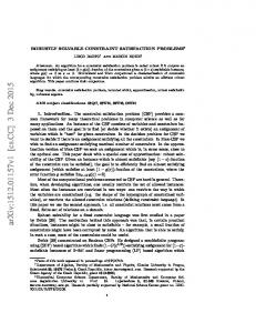
Agent-based computation has been studied for several years in the field of artificial intelligence and has been widely used in other branches of computer science. Multi-agent systems are computational systems in which several agents interact or work together in order to achieve goals. In the specialized literature, there are many works about distributed CSP. In [Yokoo et al., 1998], Yokoo et al. present a formalization and algorithms for solving distributed CSP. These algorithms can be classified as centralized methods, as synchronous backtracking and as asynchronous backtracking [Yokoo, 1995]. Our model can be considered as a synchronous model. It is meant to be a framework for interacting agents to achieve a global solution state. The main idea of our multi-agent model is based on carrying out a partition of the problem constraints, in k groups called blocks of constraints, so that the most restricted constraints are grouped and studied by autonomous agents. To this end, a preprocessing step carries out a partition of the constraints, similar to a sample in finite population, in order to classify the constraints from the most restricted ones to the least restricted ones. Then, a group of block agents manages concurrently each block of constraints, generated by the preprocessing step. Each block agent is in charge of solving its partial problem by means of a stochastic local search algorithm. Thus, finding a solution to a distributed CSP requires that all block agents find a incremental consistent partial state for their own partial problem, that is, the solution is incrementally generated from the first block agent to the last block agent. Figure 1 shows the multi-agent model, in which consistent partial states (sij ) are concurrently generated by each block agent (ai ) and sent to the following block agent until a consistent state is found (for example, state: s11 + s21 + sk1 ). Each block agent maintains the corresponding domains for its new variables and must assign values to its new variables so that the block of constraints is satisfied. When a block agent finds a value for each new variable, then it communicates with the next block agent by sending the consistent partial state. Thus, when the last block agent assigns values to the new variables that satisfy its block of constraints, then a consistent state is found.
3.1
*,+ &�- +.�� &�)/)/0 '�$21 ( &�3�4 3�5
798;:,< = >@? A :�= B ? > = A = AC8C:
3�6
��� �!�" # ��$!�&���'���( � ) %
� ��
�����
�
�
�
�
�
�
�
�
�
�
�
�
�
I/J ICK
ICL *,+.��D!� &�EF1 �G� H ( 0 � '�)
Figure 1: Multi-agent model and well distributed states (s is a polynomial function) in order to represent the entire population. As in statistic, the user selects the size of the sample (s(n)). Without loss of generality, we suppose a sample of (n2 ) states. The preprocessing step studies how many states sti : sti ≤ n2 satisfy each constraint ci . Thus, each constraint ci is labeled with pi : ci (pi ), where pi = sti /n2 represents the probability that ci satisfies the whole problem. Thus, in the preprocessing step the constraints are classified in ascending order of the labels pi . Therefore, in the preprocessing step, the initial CSP is translated into an ordered CSP so that, it can be divided into a set of subproblems. Furthermore, this sample will be used by the stochastic local search algorithms to restart the search. Thus, the random states with lower evaluation value Tsi are firstly selected to restart the search.
���� ����� � �� �� �� �� ����� � ������ ��� ��� � ��� � ����������� �� � ���
������ � �� �� �����������! � ��"�#�� � � �� � ����� ���� �� �� ��
Preprocessing Step
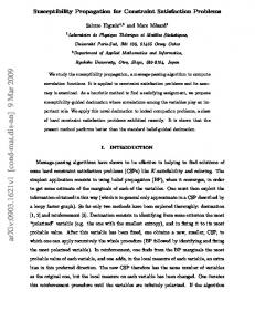
In this section, we present the preprocessing step that classifies the constraints, so that the most restricted constraints are studied first. As we pointed out above, the preprocessing step carries out a sample from a finite population in statistics, where there is a population, and a sample is chosen to represent this population. In our context, the population is composed by the states generated by means of the Cartesian Product of variable domain bounds and the sample is composed by s(n) random
Figure 2: Preprocessing step The stochastic local search algorithm moves to the neighbor and restarts at the following lower evaluation value state when a local-minimum or a number of iterations (Max-Flips) is reached. In Figure 2, an example of the preprocessing step is shown. It can be observed that a sample of states is selected from the spanning tree. Each state is checked with the prob-
lem constraints and the evaluation value Tsi is stored to be used by the stochastic local search algorithms. Furthermore, each constraint ci is labeled in order to be classified from the most restricted one to the least restricted one. Thus, as we pointed in Figure 1, these ordered constraints are partitioned in k blocks to divide the problem in k interdependent subproblems. Each problem will be solved by an agent, called block agent, using a stochastic local search algorithm and the information derived from the preprocessing step.
3.2 Block Agent
tries to find any other consistent partial state. So, each block agent j, using the variable assignment of the previous block agents 1, 2, .., j − 1, tries to find concurrently a more complete assignment. A consistent state is obtained when the last block agent k finds a complete variable assignment. Example: Let’s look at the following example, (similar to the one presented in [Yokoo et al., 1998]). There are three variables, x1 , x2 , x3 , with variable domains {1, 2, 3}, {1, 2}, {1, 2, 3}, respectively, and constraints c1 : x1 6= x2 and c2 : x2 = x3 (see Figure 4).
A block agent is a cooperating agent with a set of properties. Without loss of generality, we make the following assumptions (Figure 3):
8 8 8 6 6 7 8 8 7 8 8
G�H)IKJ L HNM O IQP)RSM T)U V P)M WNJ L P)X V
24353)6 7�8�94: 8�@4: �
� ? �
B�C � �#� ��� �$!
B�C � %&� ��� ��!
B�C � ��� �#� �#!
B�C � %#� �#� ��!
%
(
i=1
generated by the preprocessing step, and each block agent aj has a block of constraints Cj . • Each block agent aj knows a set of variables Vj involved in its block of constraints Cj . These variables fall into two different sets: used variables set (v j ) and new variables set (vj ), that is: Vj = v j ∪ vj . • The domain Di corresponding to variable xi is maintained in the first block agent at in which xi is involved, (i.e.), xi ∈ vt . • Each block agent aj assigns values (by a stochastic local search algorithm) to variables that have not been assigned yet, that is, aj assigns values to variables xi ∈ vj , because variables xk ∈ v j have already been assigned by previous agents a1 , a2 , ..., aj−1 . • Each block agent aj knows the consistent partial states generated by the previous agents a1 , a2 , ..., aj−1 . Thus, agent aj knows assignments of variables included in sets: v 1 , v 2 , ..., v j−1 . Block agents cooperate to achieve a consistent state. Block agent 1 tries to find a consistent state of its partial problem. When it has a consistent partial state, it communicates this partial state to block agent 2. Block agent 2 studies the second set of more restricted constraints using the variable assignments generated by block agent 1. Meanwhile, agent 1
) (
) ( "
� @
) (
� A �
)
#
� � � ��� %#!UTWV X"� � � �#� %�!UTW��� � � ��� �#!UTW��� � � ��� ��! Y�Z $
DFE D E F
:
' = �
!
Ci
7 8 8
� < � B�C � �"� �#� ��!
Figure 3: Block agent k S
7 8 8 : (*) +*,.� -�/ ��,#
01 �- ����
'
• There is a partition of the set of constraints C ≡
9 9
6
%
& # %
G H I J4I K�L 3NM O G H I P4I K�L 3 �I G H I J"I P�L 3 4I G H I J�I J�L QSR G H I P4I K�L 3NM O G H I J4I K�L 3 �I G H I P"I J�L 3 4I G H I P�I P�L QSR
D E F DFE
G J�I J4I J4L 3�M O G P�I J4I J4L Q�I�G K�I J4I J4L Q R G P�I P�I P4L 3 M O G J4I P�I P4L Q I4G K�I P�I P"L Q R
Figure 4: CSP solved by our model using Hill-Climbing. Only two constraints are involved, so the constraint partition is straightforward, and only two blocks, with only one constraint, are considered. The first block is composed by constraint c2 and the last block is composed by constraint c1 . This is due to the fact that constraint c2 is more restricted than constraint c1 because c2 maintains two valid tuples: (−, 1, 1) and (−, 2, 2), while c1 maintains four valid tuples: (1, 2, −), (2, 1, −), (3, 1, −) and (3, 2, −). So, block agent a1 manages constraint 1 and block agent a2 manages constraint 2. It can be observed that variables x2 and x3 are new variables in a1 and x1 is a new variable in a2 , while x2 is a used variable in a2 . Thus, domains of variable x2 and x3 are known by a1 , and the domain of x1 is known by a2 . Furthermore, a1 is responsible for assigning values to x2 and x3 , using a stochastic local search algorithm, and a2 is responsible for assigning values to x1 . Figure 4 shows the behavior of our distributed model using Hill-Climbing. It can be observed that the time step 1 is only used by a1 to generate a consistent partial state (-,1,1). Hill-Climbing starts at randomly generated state (-,1,3) with evaluation value (1) in HC1 . Its neighbors are (-,2,3),(-,1,2) and (-,1,1), with evaluation value
(1),(1) and (0), respectively. So, the neighbor with the best evaluation value is (-,1,1), which is a consistent partial state. Thus, a1 sends a message to a2 containing the consistent partial state (−, 1, 1). In time step 2, both a1 and a2 work for finding a consistent state for their own problems. a2 tries to find a value to x1 , knowing that x2 and x3 are fixed to (1,1). Hill-Climbing starts at randomly generated state (1,1,1) with evaluation value (1) in HC3 . Its neighbors are (2,1,1) and (3,1,1), with evaluation value (0) and (0), respectively. Furthermore, in time step 2, a1 tries to find another consistent partial state for x2 and x3 . Thus, in time step 2, a2 finds a value to x1 , and a consistent state (2,1,1) is reached, while a1 finds another consistent partial state (−, 2, 2) in HC2 . If only one solution is required, the process is halted. However, if more solutions are required, the process continues in time steps 3,4 and 5 using Hill-Climbing HC3 and HC4 . It can be observed (in time step 2) that our model allows agents to run concurrently to achieve consistent partial states. Let’s suppose that the domain of x1 is d1 : {1}. Then, the first consistent partial state, generated by a1 (in time step 1), is (-,1,1). It does not go through a consistent state, because there is no value to x1 (in time step 2) to satisfy the constraint c1 . Thus, the state (1, 1, 1) is a local-minimum because this state is not a solution and the evaluation values of all its neighbors are larger than or equal to the evaluation value of this state. Then, a1 restarts at another randomly generated state (-,2,3), (in time step 2), in which Hill-climbing finds a consistent partial state (-,2,2), that will go through a consistent state (1,2,2) by a2 in the time step 3.
3.3
Application to Problems with Hard and Soft Constraints
The proposed distributed model can be also applied to problems with hard constraints and soft constraints. Hard constraints are conditions that must be satisfied, soft constraints however may be violated, but should be satisfied as much as possible. This type of problems can be easily managed as following: • First, the preprocessing step studies normally the hard constraints, that is, it classifies the hard constraints so that the most restricted set of hard constraints are studied first. • Later, the preprocessing step studies the soft constraints. However, in this case, it classifies the soft constraints so that the least restricted set of soft constraints are studied first. In this way, the priority of constraints is: The most restricted hard constraints, the least restricted hard constraints, the least restricted soft constraints and the most restricted soft constraints. Thus, hard constraints must be satisfied and as many soft constraints as possible.
4
Evaluation
The n-queens problem is a classical search problem in the artificial intelligence area. The 4-queens problem is internally managed in Figure 5.
���������� ���� � ������ � � � �� ��� � ������� ��� �� � � ������� �� �� � � ������� �� �� � � ������� ��� �� � � ������� �� �� � ������� !#"$"$%�&$'('()�*+)�,�-/. �021 R 4L8(8+: SCM