Dec 9, 2010 - Stochastic Local Volatility Models: Theory and Implementation. Artur Sepp. Bank of America Merrill Lynch. University of Leicester, UK.
Stochastic Local Volatility Models: Theory and Implementation Artur Sepp Bank of America Merrill Lynch University of Leicester, UK December 9, 2010
1
Plan of the presentation 1) Hedging and volatility 2) Review of volatility models 3) Local volatility models with jumps and stochastic volatility 4) Calibration using Kolmogorov equations 5) PDE based methods in one dimension 6) PDE based methods in two dimensions 7) Illustrations
2
References Some theoretical and practical details for my presentation can be found in: 1) Sepp, A. (2007) Affine Models in Mathematical Finance: an Analytical Approach, PhD thesis, University of Tartu http://math.ut.ee/~spartak/papers/seppthesis.pdf 2) Sepp, A. (2012) An Approximate Distribution of Delta-Hedging Errors in a Jump-Diffusion Model with Discrete Trading and Transaction Costs, Quantitative Finance, 12(7), 1119-1141 http://ssrn.com/abstract=1360472
3
Volatility modelling What is important for a competitive pricing and hedging model? 1) Consistency with the observed market dynamics implies stable model parameters and hedges 2) Consistency with vanilla option prices ensures that the model fits the risk-neutral distribution implied by these prices and that the model gamma is not much different from the market implied gamma
4
Hedging and volatility I Let us consider a vanilla option and for simplicity assume zero interest rates and dividends We can find the option value U (σ)(t, S) by solving the celebrated Black-Scholes-Merton (1973) partial differential equation (PDE) with log-normal volatility parameter σ: 1 (σ) + σ 2S 2USS = 0, 2 where t is current time and S is the spot price (σ)
Ut
(1)
To delta-hedge a short-position in this option we consider the following volatilities: σi - implied volatility for computing option value U (σi)(t, S) (σ ) σh - hedging volatility for computing option delta US h (t, S) Note that σh might also include the vega adjustment, which is change in σi given change in the spot, so in general σi 6= σh 5
Hedging and volatility II The delta-hedged position at time tn: Π(tn) = S(tn)∆(σh)(tn, S(tn)) − U (σi)(tn, S(tn)) One period profit-and-loss realized over time period δtn is: δΠ(tn) = S(tn−1) + δS(tn) ∆(σh)(tn−1, S(tn−1)) − U (σi)(tn−1 + δtn, S(tn−1) + δS(tn)) − Π(tn−1) �
where δS(tn) = S(tn) − S(tn−1) and δtn = tn − tn−1
6
Hedging and volatility III Consider Taylor series of U (σi)(tn−1 + δtn, S(tn−1) + δS(tn)): U (σi)(tn−1 + δtn, S(tn−1) + δS(tn)) ≈ U (σi)(tn−1, S(tn−1))
1 (σ ) (r) i + δtnΘ (tn−1, S(tn−1)) + δS(tn)∆ (tn−1, S(tn−1)) + (δS(tn))2 Γ(r)(tn−1 2
where Θ(σi)(tn−1, S(tn−1)) is the option theta, and ∆(r)(tn−1, S(tn−1)) and Γ(r)(tn−1, S(tn−1)) are realized delta and gamma: ∂ (σi) U (t, S(tn−1)) |t=tn−1 ∂t ∂ (σi) (r) ∆ (tn−1, S(tn−1)) = U (tn−1, S) |S=S(tn) ∂S U (σi)(tn−1, S(tn)) − U (σi)(tn−1, S(tn−1)) ≈ S(tn) − S(tn−1) ∂ (r) Γ (tn−1, S(tn−1)) = ∆(r)(tn−1, S) |S=S(tn) ∂S ∆(r)(tn−1, S(tn)) − ∆(r)(tn−1, S(tn−1)) ≈ S(tn) − S(tn−1)
Θ(σi)(tn−1, S(tn−1)) =
7
Hedging and volatility IV One period realized profit-and-loss is approximated by: h
i (σ ) (r) δΠ(tn) = ∆ h (tn−1, S(tn−1)) − ∆ (tn−1, S(tn)) δS(tn)
1 (σ ) i − δtnΘ (tn−1, S(tn−1)) − (δS(tn))2 Γ(r)(tn−1, S(tn−1))
2 Note that option theta satisfies the BSM PDE:
1 Θ(σi)(t, S) = − σi2S 2Γ(σi)(t, S) 2 If the delta-hedging is rebalanced at discrete times tn, the realized profit-and-loss, P&L, Π(T ) at the option maturity is Π(T ) = +
Xh
∆(σh)(t
i (r) (tn−1, S(tn−1)) δS(tn) n−1 , S(tn−1 )) − ∆
n 1 Xh
i 2 (σ ) (r) σi Γ i (tn−1, S(tn−1)) − V (tn)Γ (tn−1, S(tn−1)) S 2(tn−1)δtn
2 n where V (tn) is the realized variance V (tn) =
1 δtn
S(tn) − S(tn−1) S(tn−1)
!2
8
Hedging and volatility V. Modelling objective A: Find a pricing and hedging model that 1) predicts the correct delta: ∆(σh)(tn−1, S(tn−1)) ≈ ∆(r)(tn−1, S(tn−1)), then the P&L will be independent from the realized price path (note that ∆(σh)(tn−1, S(tn−1)) is implied by the hedging model while ∆(r)(tn−1, S(tn−1)) represents actual change in option price observed in the market given change in the spot and associated change in implied volatility σi) 2) predicts the correct gamma: Γ(σi)(tn−1, S(tn−1)) ≈ Γ(r)(tn−1, S(tn−1)) (note that Γ(σi)(tn−1, S(tn−1)) is also implied by the hedging model while Γ(r)(tn−1, S(tn−1)) is the realized change in delta given change in spot and associated change in implied volatility σi) If the model satisfies 1) and 2), realized P&L greatly simplifies to � 1 X� 2 Π(T ) = σi − V (tn) Γ(σi)(tn−1, S(tn−1))S 2(tn−1)δtn 2 n The ”edge” comes from the spread between the implied volatility squared and the realized variance: σi2 − V (tn) 9
Volatility modelling VI. Modelling objective B If the option can be sold at implied variance σi2 that is (much) higher RT 1 than the realized variance T 0 V (t0)dt0 then Π(T ) is expected to be positive because Γ(σi)(t, S(t)) is positive for vanilla options with convex pay-offs (see Sepp (2011) for approximate distribution of Π(T )) To ”materialize” the ”edge” as the P&L, it is important to have a model that is consistent with 1) and 2) For exotic options, considerations might be more complicated as Γ(σi)(t, S(t)) and Γ(r)(t, S(t)) might change the sign and generally higher order risks need to be hedged Still, implications 1) and 2) are important for a competitive pricing and hedging model. To conclude: 1) Consistency with the observed market dynamics implies stable model parameters and hedge ratios 2) Consistency with vanilla option prices ensures that the model fits the price distribution implied by these prices and that the model gamma is not much different from the market implied gamma 10
Overview I. Black-Scholes-Merton I will start with a brief review of volatility models Black-Scholes-Merton (1973) considered log-normal model: dS(t) = µ(t)S(t)dt + σS(t)dW (t), S(0) = S,
(2)
where W (t) is the Brownian motion and µ(t) is the risk-neutral drift (typically, µ(t) = r(t) − d(t), where r(t) and d(t) are deterministic instantaneous interest and dividend rates) The constant volatility σ is independent from both the spot price and any extra factors The model is not realistic in the presence of the skew observed in the equity markets (out-of-the money puts are relatively expensive than out-of-the money calls) In practice, the BSM model is as a ”static” tool: price quotation, implied volatility parametrization, benchmarking 11
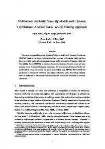
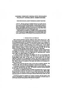
Illustration for options on the S&P 500
0.07
50%
0.06
BSM volatility, T=1month
Probability density
Implied BSM volatility
60%
Market volatility, T=1month
40%
BSM volatility, T=1year Market volatility, T=1year
30% 20% 10%
BSM density, T=1month Market density, T=1month
0.05
BSM density, T=1year Market density, T=1year
0.04 0.03 0.02 0.01
0% 0.5
0.6
0.7
0.8 0.9 1.0 1.1 1.2 K, strike=K*Forward(T)
1.3
1.4
1.5
0.00 0.00
0.22
0.43
0.65 0.86 1.08 1.29 S', spot=S'*Forward(T)
1.51
1.73
Left: Market implied and BSM volatility at ATM strike for T =1month an T =1year Right: Corresponding market and BSM implied probability density Market implied distribution is more skewed to the left 12
Overview II. Bachelier model, A Bachelier (1900) proposed a normal dynamics: dS(t) = µ(t)S(0)dt + σnormalS(0)dW (t), S(0) = S,
(3)
The implied local log-normal volatility σloc(S(t)) (approximately): S(0) σloc(S(t)) = σnormal S(t) The Bachelier model produces the leverage effect: for small price the volatility increases and vice versa The non-zero probability of negative prices: the default event in the financial terms (modelled as the first time S(t) hits zero)
13
Overview II. Bachelier model, B From the modelling point of view, the Bachelier model is more realistic than that of Black-Scholes-Merton However, the model is little accepted in practice: people prefer to think in relative terms rather than in absolute In Bachelier model, we cannot compare risks of stock A with the volatility of 100, 000% and stock B with the volatility of 10% without looking at their spot prices Now: stock A is the FTSE100 index with S(0) = 5, 700 and stock B is a penny share with S(0) = 0.1 The equivalent log-normal volatility of A is 17.54% and that of B is 100.00% 14
Overview III. Jump-diffusion models Merton (1976) introduced log-normal dynamics with normal jumps: �
� J dS(t) = µ(t)S(t−)dt + σS(t−)dW (t) + (e − 1)dN (t) − λνdt S(t−)
(4) where N (t) is a Poisson process with intensity λ, J is jump amplitude with PDF $(J) = n(η, δ), and ν is the compensator: ν=
Z ∞ −∞
0
1 2
eJ $(J 0)dJ 0 − 1 = eη+ 2 δ − 1
Given jump in N (t), jump in S(t) is: ∆S(t) = S(t−)(eJ − 1) ≈ S(t−)J Since the possibility of large jumps makes out-of-the-money puts more expensive, jump-diffusions introduce the implied volatility skew However, for longer periods (more than one year) the implied distribution resembles to the Gaussian (by the central limit theorem) Jump models have been extended to general Levy processes (Lewis (2001), Levendorskii-Boyarchenko (2002), Carr et al (2003), ContTankov (2004), ...) 15
Overview IV. Stochastic volatility models Hull-White (1988): dS(t) = µ(t)S(t)dt + V (t)S(t)dW (1)(t) dV (t) = κ(θ − V (t))dt + �V (t)dW (2)(t) where < dW (1)(t), dW (2)(t) >= ρdt Scott (1987): dS(t) = µ(t)S(t)dt + eV (t)S(t)dW (1)(t) dV (t) = κ(θ − V (t))dt + �dW (2)(t) Stein-Stein (1991): dS(t) = µ(t)S(t)dt + V (t)S(t)dW (1)(t) dV (t) = κ(θ − V (t))dt + �dW (2)(t) Heston (1993): dS(t) = µ(t)S(t)dt +
q
V (t)S(t)dW (1)(t) q
dV (t) = κ(θ − V (t))dt + � V (t)dW (2)(t) Jumps can be included (Bates (1996), Duffie et al (2000), ...) 16
Overview V. Parametric local volatility Cox (1975) proposes the constant elasticity of the variance (CEV) model: �
� β−1 dS(t) = µ(t)S(S)dt + σcev S (t) S(t)dW (t)
(5)
Rubinstein (1983) proposes the dis-placed diffusion model !
dS(t) = µ(t)S(t)dt + σdis β + γ
S(0) S(t)dW (t) S(t)
(6)
Both the CEV with β < 1 (typically, β ∈ [−5, −3] for single stocks and indexes) and dis-placed diffusions exhibit the leverage effect and the default possibility (from my experience, the dis-placed diffusion model is easier to deal with) Ingersoll (1996), Zuhlsdorff (1999) and Lipton (2000) consider the hyperbolic volatility: !
S(0) S(t) +β+γ S(t)dW (t) dS(t) = µ(t)S(S)dt + σhyp α S(0) S(t)
(7)
17
Overview VI. Non-parametric local volatility In general, parameters of parametric local volatility models need to be calibrated to observed market prices in least squares sense Derman-Kani (1994), Rubinstein (1994), Dupire (1994) consider the one-dimensional diffusion model dS(t) = µ(t)S(t)dt + σ(loc)(t, S(t))S(t)dW (t),
(8)
with local volatility σ(loc)(t, S(t)) implied from observed market prices of vanilla options Andersen-Andreasen (2000) and Carr et al (2004) introduce the local volatility with jumps JP Morgan (1999) and Blacher (2001) consider the local volatility model with stochastic variance driven by the Heston model Lipton (2002) introduces the local stochastic volatility with jumps Let me summarise the two main categories of the models used in practice for exotic options 18
Overview VII. Volatility models 1) Non-parametric local volatility models (Dupire (1994), DermanKani (1994), Rubinstein (1994)) ”+” are consistent with today’s market prices by construction ”-” but they tend to be poor in replicating the market dynamics of spot and volatility (implied volatility tends to move too much given a change in the spot, no mean-reversion effect) ”-” especially, it is impossible to tune-up the volatility of the implied volatility as there is simply no parameter for that! 2) Parametric stochastic volatility models (Heston (1993)) ”+” tend to be more in line with the market dynamics ”+” equipped to model the term-structure (by mean-reversion parameters) and the volatility of the variance (by vol-of-vol parameters) ”-” need a least-squares calibration to today’s option prices ”-” unfortunately, any change in any of the parameters of the meanreversion or the vol-of-vol requires re-calibration of other parameters 3) Stochastic local volatility models (JP Morgan (1999), Blacher (2001), Lipton (2002)) aim to include ”+”’s and cross ”-”’s of the first two models 19
Overview VIII. Model specification 1) Global factors Select factors relevant for product risk: stochastic volatility, stochastic interest rate, jumps, default risk, etc (Guess) Estimate or calibrate model parameters for the dynamics of these factors using either historical or market data Parameters are updated infrequently 2) Local factors Specify local factors such as local volatility or local drift (for quantos) Parameters of local factors are updated frequently (on the run) 20
Stochastic local volatility models Stochastic local volatility models allow: 1) Specify the dynamics for the instantaneous volatility 2) Fit the risk-neutral distributions implied by market prices of vanilla options by specifying local volatility as function of the spot price However, the model calibration requires robust numerical methods for solving two-dimensional PDE-s In general, a successful implementation of the model involves a decent amount of both theoretical and practical exercises
21
Calibration of parametric models I. Forward-backward equations I apply the methods for stochastic processes and partial differential equations dating back to Kolmogorov foundational work (1931) Consider a 1-d problem with stochastic factor S(t) for a product that depends only on terminal value of S(T ) PV function U (t, S; T, K), 0 ≤ t ≤ T , solves the backward equation as function of (t, S): Ut(t, S) + LU (t, S) = −c(t, S), U (T, S) = u(S)
(9)
u(S) and c(t, S) are pay-off and coupon functions, respectively L is the infinitesimal operator corresponding to the dynamics of S(t) (includes volatility, drift, discounting, jumps) Transition probability density function, G(0, S0; t, S 0), aka Green’s function in mathematical physics, solves the forward equation as function of (t, S 0): Gt(t, S 0) − L†G(t, S 0) = 0, G(0, S 0) = δ(S 0 − S0)
(10)
where δ() is Dirac delta function and L† is operator adjoint to L 22
Calibration of parametric models II. Valuation formula Multiply backward equation by G(0, S0; t, S) and integrate over (t, S): Z TZ ∞
−
0 −∞ Z TZ ∞ h
≡ = −
Z0∞ −∞ h
−∞ Z T
= −
G(0, S0; t0, S 0)c(t0, S 0)dS 0dt0 i 0 0 0 0 0 0 0 0 G(0, S0; t , S )Ut(t , S ) + G(0, S0; t , S )LU (t , S ) dS 0dt0
G(0, S0; T, S 0)U (T, S 0) − G(0, S0; 0, S 0)U (0, S 0) #
Gt(0, S0; t0, S 0)U (t0, S 0)dt0 dS 0 +
0 Z ∞
−∞ 0
G(0, S0; t0, S 0)LU (t0, S 0)dt0dS 0
G(0, S0; T, S 0)u(S 0)dS 0 − U (0, S0)
−∞ Z T Z ∞ hn 0
Z ∞ Z T
−∞
o n oi † 0 0 0 0 0 0 0 0 L G(0, S0; t , S ) U (t , S ) − G(0, S0; t , S ) LU (t , S ) dS 0dt0
where, in second line, the first term is integrated by parts, and, in the last line, terminal condition for U (T, S) and initial condition for G(0, S0; 0, S) are applied 23
Calibration of parametric models III. Consistency Consistency condition for adjoint operators L and L† (can be checked by integration by parts): Z T Z ∞ hn 0
−∞
o n oi † 0 0 0 0 0 0 0 0 L G(0, S0; t , S ) U (t , S ) − G(0, S0; t , S ) LU (t , S ) dS 0dt0 = 0
(11) Then the PV can be computed by convolution: U (0, S0; T, K) = +
Z ∞
G(0, S0; T, S 0)u(S 0)dS 0
−∞ Z TZ ∞ 0
−∞
(12) G(0, S0; t0, S 0)c(t0, S 0)dS 0dt0
This formula is known as Duhamel’s principle (19th century) in mathematical physics or Feynman-Kac formula (1949) in probability
24
Calibration of parametric models IV. Implications Typically, for a parametric model, model parameters are assumed to be piece-wise constant in time with jumps at times {Tn}, where {Tn} is set of maturity times of listed options Implications for calibration by bootstrap: 1) Given calibrated set of piece-wise constant model parameters at time Tm−1 and known values of G(Tm−1, S), make a guess for parameters at time Tm and compute G(Tm, S) 2) Apply Duhamel’s formula (12) to compute PV-s of specified vanilla instruments 3) By changing parameters for time Tm, minimize the sum of squared differences between model and market prices 4)After convergence, store G(Tm, S) and go to the next time slice 25
Calibration of parametric models V. Numerical schemes Consistency condition (11) for adjoint operators L and L† is based on theoretical arguments: Z T Z ∞ hn 0
−∞
o n oi † 0 0 0 0 0 0 0 0 L G(0, S0; t , S ) U (t , S ) − G(0, S0; t , S ) LU (t , S ) dS 0dt0 = 0
It is not necessarily true for discrete numerical schemes! (see Lipton (2007) for a consistent scheme) Implications for numerical schemes: 1) For adjoint operators, if M is spacial discretisation of L then M T should be spacial discretisation of L† 2) Both forward and backward equations should be solved using the same schemes 3) It is enough to develop either forward or backward scheme 4) L and L† have the same values of the operator norm, so the convergence of the forward scheme implies convergence of the backward scheme and vice versa 26
Local volatility calibration I. Basic facts Let G(t, S; T, S 0) be the risk-neutral probability density at time T and state S 0 given that S(t) = S: h i 0 0 G(t, S; T, S ) = P S(T ) ∈ dS | S(t) = S dS 0
(13)
Assume that the discount rate is deterministic By applying the risk-neutral valuation and Duhamel’s formula (12), un-discounted call value C(T, K) solves: C(T, K) = =
Z ∞ Z0∞ K
(S 0 − K)+G(t, S; T, S 0)dS 0 (S 0 − K)G(t, S; T, S 0)dS 0
(14)
By basic calculus: CK (T, K) = −
Z ∞ K
G(t, S; T, S 0)dS 0
(15)
CKK (T, K) = G(t, S; T, K) 27
Local volatility calibration II. Breeden-Litzenberger formula Consider a one-dimensional diffusion: dS(t) = µ(t)S(t)dt + σ(loc,dif)(t, S(t))S(t)dW (t), S(0) = S
(16)
where σ(loc,dif) is the local volatility of the diffusion Note that if call prices are given for all strikes and maturities, {C (market)(K, T )}, then by (15) the risk-neutral distribution satisfies (Breeden-Litzenberger (1978)): (market)
G(market)(T, K) = CKK
(T, K)
Calibration objective: how we should specify σ(loc,dif)(T, S 0) so that the implied risk-neutral distribution G(t, S; T, S 0) is consistent with G(market)(T, K) 28
Local volatility calibration III. Kolmogorov equation The risk-neutral probability density G(t, S; T, S 0) solves the forward Kolmogorov equation: � � � 1� 0 0 2 0 GT − (σ(loc,dif)(T, S )S ) G 0 0 + µ(T )S G 0 = 0 SS S 2 G(t, S; t, S 0) = δ(S 0 − S)
Multiply by (S 0 − K)+ and integrate over S 0 Initial condition: Z ∞ 0
(S 0 − K)+δ(S 0 − S)dS 0 = (S − K)+
Time derivative: Z ∞ 0
(S 0 − K)+GT dS 0 = CT (T, K) 29
Diffusion term: Z ∞
� � 0 + 0 0 2 2 (S − K) (σ(loc,dif)(T, S )S ) G 0 0 dS 0 = σ(loc,dif) (T, K)K 2G(t, S; T, K) SS 0 2 = σ(loc,dif) (T, K)K 2CKK (T, K)
Drift term: Z ∞
� � 0 + 0 (S − K) µ(T )S G 0 dS 0 = µ(T )KCK (T, K) − µ(T )C(T, K) S 0
As a result, we obtain the forward equation for call option prices as function of the ”forward” arguments T and K: 1 2 (T, K)K 2CKK + µ(T )KCK − µ(T )C = 0 CT − σ(loc,dif) 2 C(t, K) = (S(t) − K)+ 2 Inverting the PDE in terms of the σ(loc,dif) , we obtain Dupire equation (1994) for local volatility: 2 σ(loc,dif) (T, K) =
CT (T, K) + µ(T )KCK (T, K) − µ(T )C(T, K) 1 K 2C KK (T, K) 2
(17) 30
Jump-diffusion model I Andersen-Andreasen (2000) consider a Merton jump-diffusion extended to local volatility: dS(t) =µ(t)S(t−)dt + σ(loc,jd)(t, S(t−))S(t−)dW (t) �
� J + (e − 1)dN (t) − λνdt S(t−), S(0) = S
(18)
where σ(loc,jd) is the local volatility corresponding to the jump-diffusion
31
Jump-diffusion model II Kolmogorov equation Now G(t, S; T, S 0) solves the forward Kolmogorov equation: � � � 1� 0 0 2 0 GT − (σ(loc,jd)(T, S )S ) G 0 0 + µ(T )S G 0 − λI(S 0) = 0 SS S 2 G(t, S; t, S 0) = δ(S 0 − S)
I(S 0) =
Z ∞ −∞
0
0
G(S 0e−J )e−J $(J 0)dJ 0 + (νS 0G)S 0 − G
Proof: for the backward equation the jump term is given by: I ?(S 0) =
Z ∞ −∞
0 0 J U (S e )$(J 0)dJ 0 − νS 0US 0 − U
Multiply by G(t, S; T, S 0) and integrate over S 0: Z ∞
G(t, S; T, S 0)I ?(S 0)dS 0 =
−∞ Z ∞
−
=
νG(S 0)S 0US 0 dS 0 −
Z−∞ ∞ �Z ∞ −∞
−∞
Z ∞
Z ∞ −∞
0
G(t, S; T, S 0)U (S 0eJ )$(J 0)dJ 0dS 0
GU dS 0
−∞ � 0 0 G(t, S; T, S 0e−J )e−J $(J 0)dJ 0 + (νS 0G)S 0 − G U (S 0)dS 0 0
by making substitution S 0eJ → S 0 and integrating by parts 32
Jump-diffusion model IV Following the same steps consider: I †(K) = = =
Z ∞ Z0∞
Z ∞ 0
(S 0 − K)+I(S 0)dS 0
(S 0 − K)+
−∞
Z ∞
0
0
G(S 0e−J )e−J $(J 0)dJ 0dS 0 + νKCK − (ν + 1)C
−∞ 0 J0 −J C(Ke )e $(J 0)dJ 0 + νKCK − (ν + 1)C
As a result, obtain the forward equation for call option prices: 1 2 CT − σ(loc,jd)(T, K)K 2CKK + µ(T )KCK − µ(T )C − λI †(K) = 0 2 C(t, K) = (S(t) − K)+ 2 Inverting σ(loc,jd) yields Andersen-Andreasen equation (2000):
CT (T, K) + µ(T )KCK (T, K) − µ(T )C(T, K) − λI †(K) 2 σ(loc,jd)(T, K) = 1 K 2C KK (T, K) 2 λI †(K) 2 = σ(loc)(T, K) − 1 2 2 K CKK (T, K) 33
Stochastic local volatility I Consider 2-d stochastic local volatility diffusion: dS(t) = µ(t)S(t)dt + σ(loc,sv)(t, S(t))ϑ(t, Y (t))S(t)dW (1)(t), S(0) = S, dY (t) = θ(Y (t))dt + �(Y (t))dW (2)(t), Y (0) = Y (19) where σ(loc,sv) is the local volatility of the diffusion with stochastic volatility and < dW (1)(t), dW (2)(t) >= ρdt ϑ(t, Y (t)) is the mapping function of Y (t) into the spot dynamics
34
Stochastic local volatility II. Calibration Conventional approach (for example, Ren-Madan-Qian (2007)) is to use Gy¨ ongy (1986) mimicking theorem yielding: h i 2 2 2 σ(loc,sv)(T, K)E ϑ (T, Y (T )) | S(T ) = K = σ(loc,dif) (T, K)
Gy¨ ongy theorem is purely probabilistic analysis, we follow original Lipton’s (2002) PDE-based approach applied directly in the context of stochastic local volatility calibration The risk-neutral probability density G(t, S, Y ; T, S 0, Y 0) solves the forward Kolmogorov equation: � � � 1� 0 0 0 2 0 GT − (σ(loc,sv)(T, S )ϑ(T, Y )S ) G 0 0 + µ(T )S G 0 SS S 2 � � � � 1 2 0 − � (Y )G 0 0 + θ(Y 0)G 0 Y Y Y 2 � � 0 0 0 0 − ρσ(loc,sv)(T, S )ϑ(T, Y )�(Y )S G 0 0 = 0
G(t, S, Y ; t, S 0, Y 0) = δ(S 0 − S)δ(Y 0 − Y )
SY
35
Stochastic local volatility III. Calibration Consider the unconditional density: U (t, S; t, S 0) =
Z ∞ −∞
G(t, S, Y ; T, S 0, Y 0)dY 0
The diffusion term becomes: Z ∞ �
(σ(loc,sv)
−∞ ��Z ∞
(T, S 0)ϑ(T, Y 0)S 0)2G
� S 0S
0 dY 0
�
ϑ2(T, Y 0)GdY 0 (σ(loc,sv)(T, S 0)S 0)2 −∞
=
= V (T, S 0)(σ(loc,sv)(T, S 0)S 0)2U (T, S 0) �
� S 0S 0
� S 0S 0
where V (T, S 0) is the conditional variance: R∞ 2 (T, Y 0 )G(t, S, Y ; T, S 0 , Y 0 )dY 0 ϑ V (T, S 0) = −∞ U (t, S; T, S 0) R∞ 2 0 0 0 0 −∞ ϑ (T, Y )G(t, S, Y ; T, S , Y )dY = R∞ 0 0 0 −∞ G(t, S, Y ; T, S , Y )dY 36
Stochastic local volatility IV. Calibration Remaining terms are trivial, yielding: � � � 1� 0 0 0 2 0 UT − V (T, S )(σ(loc,sv)(T, S )S ) U 0 0 + µ(T )S U 0 = 0 SS S 2 U (t, S; t, S 0) = δ(S 0 − S)
PDE for call prices: 1 CT − (V (T, K)(σ(loc,sv)(T, K)K)2CKK + µ(T )KCK − µ(T )C = 0 2 The model is consistent with the Dupire local volatility if 2 2 V (T, K)σ(loc,sv) (T, K) = σ(loc,dif) (T, K)
As a result, the stochastic local volatility is specified by: 2 σ(loc,sv) (T, K) =
2 σ(loc,dif) (T, K)
V (T, K) 37
Stochastic local volatility with jumps I Consider a two-dimensional stochastic local volatility jump-diffusion: dS(t) =µ(t)S(t−)dt + σ(loc,svj)(t−, S(t−))ϑ(t−, Y (t−))S(t−)dW (1)(t) �
� J + (e − 1)dN (t) − λνdt S(t−), S(0) = S,
dY (t) =θ(Y (t))dt + �(Y (t))dW (2)(t) + ΥdN (t), Y (0) = Y (20) where σ(loc, svj) is the local volatility of the diffusion with stochastic volatility and jumps Υ is the amplitude of the jump in Y (t) with PDF ς(Υ) Jumps are simultaneous in S(t) and Y (t)
38
Stochastic local volatility with jumps II The risk-neutral probability density G(t, S, Y ; T, S 0, Y 0) solves the forward Kolmogorov equation: � � � 1� 0 0 0 2 0 GT − (σ(loc,svj)(T, S )ϑ(T, Y )S ) G 0 0 + µ(T )S G 0 SS S 2 � � � � 1 2 0 − � (Y )G 0 0 + θ(Y 0)G 0 Y Y Y 2 � � 0 0 0 0 − ρσ(loc,svj)(T, S )ϑ(T, Y )�(Y )S G 0 0 − λI(S 0) = 0
I(S 0) =
Z ∞ Z ∞
SY G(S 0e−J , Y 0 − Υ)e−J $(J)ς(Υ)dJdΥ + (νS 0G)S 0 − G
−∞ −∞ 0 G(t, S, Y ; t, S , Y 0) = δ(S 0 − S)δ(Y 0 − Y )
39
Stochastic local volatility with jumps III PDE for call prices: 1 CT − (V (T, K)(σ(loc,svj)(T, K)K)2CKK + µ(T )KCK − µ(T )C − λI †(K) = 0 2 where V (T, K) is the unconditional variance 2 Inverting σ(loc,svj) (T, K), yields Lipton equation (2002):
CT (T, K) + µ(T )KCK (T, K) − µ(T )C(T, K) − λI †(K) 2 σ(loc,svj)(T, K) = 1 V (T, K)K 2 C KK (T, K) 2 † λI (K) 1 σ 2 = (T, K) − (loc,dif) 1 2 V (T, K) 2 K CKK (T, K) 2 σ(loc,jd) (T, K) =
V (T, K) 40
PDE based methods Non-parametric local stochastic volatility can only be implemented using numerical methods for partial integro-differential equations These methods should be flexible to handle jumps in one and two dimensions and the correlation term for two dimensions I will review some of the available methods For the backward problem, L is the infinitesimal operator corresponding to model dynamics: L = D + λJ
41
1-d Problem Here D is the diffusion-convection operator: 1 2 DU (t, S) ≡ σ (t, S)S 2USS + µ(t)SUS + λU 2 J is the integral operator: J U (t, S) ≡
Z ∞ −∞
0 J U (t, Se )$(J 0)dJ 0
For the forward problem, we consider the operator L† adjoint to L: L† = D† + λJ † For both problems we denote the discretized diffusion and integral operators by Dn and J, respectively The diffusion operator is space and time dependent (denoted by n) Care must be taken for discretization of the operator for the meanreverting process! 42
1-d Problem for diffusion problem I N - number of points in the space grid Dn - discrete diffusion matrix at time tn with dimension N × N U n - the solution vector at time tn with dimension N × 1 I - the unit matrix with dimension N × N Time-stepping methods of the choice: Explicit method: U n+1 =
�
� n+1 I+D Un
Implicit method: �
� n+1 I−D U n+1 = U n
θ method: �
� � � n+1 n+1 n+1 I − θD U = I + θD Un
with θ = 1 2 corresponding to Crank-Nicolson scheme 43
1-d Problem for diffusion problem II The explicit method requires very fined grids and is highly unstable it should be avoided The Crank-Nicolson scheme is unconditionally stable and is of order (δS)2 and (δt)2, but might lead to negative probabilities for the forward equation The implicit method is unconditionally stable and does not lead to negative densities, but it is of order (δt) and becomes less accurate for longer maturities My favourite is the predictor-corrector scheme: �
� n+1 e = Un I−D U � � 1 n+1 n n+1 n+1 n e) (U − U I−D U =U + D
2 which is of order (δS)2 and (δt)2, and does not lead to negative probabilities 44
Numerics for jump-diffusions I Let me consider the forward equation with additive jumps (multiplicative jumps can be handled in the log-space): J G(x) =
Z ∞ −∞
G(x − j)$(J 0)dJ 0
Let me consider discrete negative jumps with size −η, η > 0: J G(x) = G(x + η) Discretization is a simple linear interpolation: J Gi = wGk + (1 − w)Gk+1 where k = min{k : xk+1 ≥ xi + ν} and w =
xk+1 −(xi +ν) xk+1 −xk
45
Numerics for jump-diffusions II In the matrix form, for uniform spacial grid:
J
=
0 0 ... 0 0 ... 0
0 ... w 1 − w 0 ... 0 0 ... 0 w 1 − w ... 0
0 0
0 ... 0 0 ... 0
0 0
0 0
... w 1 − w ... 0 1
0 ... 0
0
0
... 0
0
J(p,N ) = 1, where p = min{p : xp + ν ≥ xN } In general, for two-sided jumps, J is a full matrix: The implicit method for the integral term leads to O(N 3) complexity and is not practical The explicit method leads to O(N 2) complexity but needs extra care for stability For exponential jumps, Lipton (2003) develops recursive scheme with O(N ) complexity 46
Numerics for jump-diffusions III In case of discrete jumps, we have two-banded matrix with p rows that have non-zero elements Consider solving a linear system: (I − β J)X = R where β = λδt, 0 < β < 1 We can solve this system by back-substitution with cost of O(N ) operations
47
Numerics for jump-diffusions IV Consider θ and θJ schemes for the diffusion and the jump parts: �
� � � n+1 n+1 n+1 I − θD − θJ λn+1J U = I + θD + θJ λn+1J U n
where λn+1 = (tn+1 − tn)λ(tn+1) 1 is supposed to be O(dx2 ) + O(dt2 ) The accuracy with θ = θJ = 2 However, the matrix in the lhs will be full: the cost to invert is O(N 3) Implicit-explicit method: �
� � � n+1 n+1 I−D U = I + λn+1J U n
with accuracy of O(dx2) + O(dt) θ-explicit method: �
� � � n+1 n+1 n+1 I − θD U = I + θD + λn+1J U n
with accuracy of O(dx2) + O(dt) 48
Numerics for jump-diffusions V. Andersen-Andreasen (2000) scheme Make the first half step with θ = 1 and θJ = 0 and the second half step with θ = 1 and θJ = 1: 1 1 I − Dn+1 Ue = I + λn+1J U n 2 � � �2 � 1 1 I − λn+1J U n+1 = I + Dn+1 Ue 2 2 �
�
�
�
with accuracy of O(dx2) + O(dt2) When J is full, the second equation can be solved by the application of the discrete Fourier transform (DFT) with the cost of O(N log N ) For discrete jumps, the second equation solved with cost of O(N ) operations 49
Numerics for jump-diffusions VI. d’Halluin et al (2005) scheme Consider fixed point iterations: Set V 1 = U n Iterate for p = 1, .., p (p = 2 is good enough): �
� � � n+1 p+1 n+1 I − θD V = I + θD U n + λn+1JV p,
Set U n+1 = V p The accuracy is O(dx2) + O(dt)
50
Numerics for jump-diffusions VII My favourite is the implicit scheme with predictor-corrector applied twice: � � (0) n+1 e U = I+D + λn+1J U n � � n+1 e =U e (0) I−D U � 1 n+1 n+1 n+1 (0) e − U n) e + λn+1J)(U I−D U =U + (D
�
2
The accuracy is O(dx2) + O(dt2)
51
Numerical Methods for Two Dimensional Problem I We consider the forward problem for U (t, x1, x2): UT − MU = 0 U (0, x1, x2) = δ(x1 − x1(0))δ(x2 − x2(0))
(21)
where M = D1 + D2 + C + λJ D1 and D2 are 1-d diffusion-convection operators in x1 and x2 directions, respectively C is the correlation operator J is the integral operator for joint jumps in x1 and x2 Let D1 and D2 denote the discretized 1-d diffusion-convection operators in x1 and x2 directions, respectively
C and J are the discretized correlation and integral operator, respectively 52
Douglas-Rachford (1956) scheme Make a predictor and apply two orthogonal corrector steps: e (0) = (I + C + λJ + D + D )U n U 1 2 e =U e (0) − θ D U n (I − θD1)U 1 e − θD U n (I − θD2)U n+1 = U 2
In the second line, for each fixed index j we apply the diffusion operator in x1 direction; and solve the tridiagonal system of equations to e (·, x (j)) get the auxiliary solution U 2 In the third line, keeping i fixed, we apply the diffusion step in x2 direction and solve the system of tridiagonal equations to get the solution U n+1(x1(i), ·) at time tn+1 Complexity is O(N1N2) per time step 53
Craig-Sneyd (1988) scheme Start as with Douglas-Rachford scheme make a second predictor and again apply two orthogonal corrector steps: e (0) = (I + C + λJ + D + D )U n U 1 2 e (1) = U e (0) − θ D U n (I − θD1)U 1 e (2) = U e (1) − θ D U n (I − θD2)U 2 1 (3) (0) e e e (2) − U n) U =U + (C + λJ)(U 2 e (4) = U e (3) − θ D U n (I − θD1)U 1 e (4) − θ D U n (I − θD2)U n+1 = U 2
54
Hundsdorfer-Verwer (2003) scheme (in’t Hout-Foulon (2008)) Similar to Craig-Sneyd scheme with predictor including D1 and D2 e (2): and the second corrector applied on U e (0) = (I + C + λJ + D + D )U n U 1 2 e (1) = U e (0) − θ D U n (I − θD1)U 1 e (2) = U e (1) − θ D U n (I − θD2)U 2 � � 1 (2) n (3) (0) e e e −U U =U + (C + λJ + D1 + D2) U 2 e (4) = U e (3) − θ D U e (2) (I − θD1)U 1 e (4) − θ D U e (2) (I − θD2)U n+1 = U 2
55
Discretisation of integral term Direct methods are infeasible because of O(N12N22) complexity DFT method (Clift-Forsyth (2008)) has O(N1N2 log N1N2) complexity but suffers from problems associated with the DFT Explicit methods with O(N1N2) complexity are available for discrete and exponential jumps (Lipton-Sepp (2011)) The simplest case is if jumps are discrete with sizes η1 and η2: J G = G(x1 − η1, x2 − η2) This term is approximated by bi-linear interpolation with the second order accuracy leading to the O(N1N2) complexity 56
Illustration I. Model specification We specify a particular version of the LSV dynamics (20): dS(t) = µ(t)S(t−)dt + σ(loc,svj)(t−, S(t−))ϑ(t−, Y (t−))S(t−)dW (1)(t) � −ν + (e − 1)dN (t) + λνdt S(t−), S(0) = S �
dY (t) = −κY (t)dt + �dW (2)(t) + ηdN (t), Y (0) = 0 (22) where dW (1)(t)dW (2)(t) = ρdt Convenient choice of ϑ(t, Y (t)): ϑ(t, Y (t)) = eY (t)−V[Y (t)] where V[Y (t)] is the variance of Y (t). Then if ρ = 0: h
i 2 E ϑ (t, Y (t)) | Y (0) = 0 = 1
Mapping ϑ(t, Y (t)) introduces the ”volatility-of-volatility” effect without affecting the local volatility close to the spot Simultaneous jumps in S(t) and Y (t) are discrete with magnitudes −ν < 0 and η > 0 (note that jump variance will decrease the model implied correlation between spot and volatility) 57
Illustration II. Model calibration
1) Specify time and space grids 2) Compute the local volatility using Dupire equation (17) on the specified grid (interpolating implied volatilities in strikes and maturities) 3) Calibrate local stochastic volatility on the specified grid 4) Use backward PDE methods or Monte-Carlo simulations of the local stochastic volatility model to compute values of exotic options
58
Illustration III. Local volatility calibration A At initial time t0 = 0 i) initialize G0(x1(i), x2(j)) = 1x1(i)=x1(t0)1x2(j)=x2(t0) ii) Set the conditional variance V (t1, x1(i)) = 1 so that 2 2 σ(loc,sv) (t1, x1(i)) = σ(loc,dif) (t1, x1(i))
iii) Compute G1(x1(i), x2(j)) by solving the forward PDE iv) Compute V (t1, x1(i)) by P P 2 1 i j ϑ (t1 , x2 (j))G (x1 (i), x2 (j)) V (t1, x1(i)) = P 1 j G (x1 (i), x2 (j))
and set 2 σ(loc,sv) (t1, x1(i)) =
2 σ(loc,dif) (t1, x1(i))
V (t1, x1(i))
G) Repeat C) and D) and go to the next time step 59
Illustration III. Local volatility calibration B At time tn given Gn−1(x1(i), x2(j)) and V (tn−1, x1(i)) i) Compute the local variance by: 2 σ(loc,sv) (tn, x1(i)) =
2 σ(loc,dif) (tn, x1(i))
V (tn−1, x1(i))
ii) Compute Gn(x1(i), x2(j)) by solving the forward PDE iii) Compute V (tn, x1(i)) by P P 2 n i j ϑ (tn , x2 (j))G (x1 (i), x2 (j)) V (tn, x1(i)) = P n j G (x1 (i), x2 (j))
and set 2 σ(loc,sv) (tn, x1(i)) =
2 σ(loc,dif) (tn, x1(i))
V (tn, x1(i))
D) Repeat B) and C) and go to the next time step 2 For stochastic volatility with jumps we use σ(loc,jd) 60
Illustration III. Local volatility calibration C When we use predictor-corrector schemes: i) Compute the predictor step using local stochastic volatility from previous time step ii) Update local stochastic volatility and compute the corrector step with new volatility iii) After the corrector step, compute new local stochastic volatility and go to the next step
61
Illustration IV. Discrete dividends At ex-dividend time tn: S(tn+) = S(tn−) − Dn where Dn is the cash dividend at time tn Note that this corresponds to the negative jump in S(t) with a constant magnitude Dn at deterministic time tn Therefore the developed method for discrete negative jumps are readily applied for discrete dividends 2 It is important that σ(loc,dif) is consistent with the discrete dividends
62
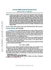
Illustration V. Local volatilities for options on the S&P 500
70%
80% Dupire Local Volatility, T=1year
Dupire Local Volatility, T=1month
60%
70%
50%
Local Volatility
Local Volatility
SV Local Volatility, T=1month
40% 30% 20% 10%
SV Local Volatility, T=1year
60% 50% 40% 30% 20% 10%
0%
0% 0.2
0.2
0.3
0.3 0.4 0.5 0.6 0.8 S', spot = S'*forward(T)
1.0
1.2
0.2
0.2
0.3
0.3 0.4 0.5 0.6 0.8 S', spot = S'*forward(T)
1.0
1.2
Left: Dupire local volatility and LSV local volatilities at T=1 month Right: ... at T=1 year LSV local volatility is an adjustment to the skew implied by the stochastic volatility part and is mostly flat 63
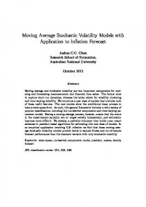
Illustration VI. Forward volatilities for options on the S&P 500
55% 50%
Implied BSM volatility
Implied BSM volatility
6m Spot skew, Local vol 6m Spot skew, LSV
45%
6m-6m Skew if S(6m)>1.1S(0), Local vol
40%
6m-6m Skew if S(6m)>1.1S(0), LSV
35% 30% 25% 20%
60%
6m Spot skew, Local vol
55%
6m Spot skew, LSV
50%
6m-6m Skew if S(6m) 1.1S(0) Right: 6m-6m skew if S(T = 6m) < 0.9S(0): the implied volatility for the forward-start option conditional that S(T = 6m) < 0.9S(0) 64
Illustration VII. Implications Conditional that spot moves up, the LSV model preserves the shape of the volatility skew while the pure local volatility does not Conditional that spot moves down, the pure local volatility implies that the ATM volatility goes too high and the skew flattens unlike the LSV model The LSV is more closer to the actual dynamics!
65
Illustration VIII. Implied volatilities of options on the daily realized variance of the S&P 500
120%
160% 120% LSV, T=3m
80%
Local Vol, T=3m
40% 0% 23%
58%
92%
127% 162% 196% 231%
K, Strike=K*ExpectedVariance(T)
Implied log-normal voltility
Implied log-normal voltility
200%
80%
40% LSV, T=1year Local Vol, T=1year
0% 15%
37%
59%
81%
103%
125%
147%
K, Strike=K*ExpectedVariance(T)
Left: Implied log-normal volatilities on options on the daily realized variance of the S&P 500 with maturity T=3 month Right: ... at T=1 year LSV local volatility implies higher volatility of the realized variance ad the vol-of-vol parameter can be ”tuned-up” to match the market 66
Illustration IX. Options on the VIX Augment the model dynamics (22) with the third variable for the realized quadratic variance of S(t): �2
�
dI(t) = σ(loc,svj)(t−, S(t−))ϑ(t−, Y (t−))
dt + ν 2dN (t), I(0) = 0
Consider the expected variance realized over period [T, T + Tvix]: e I(T, T + Tvix) =
1 E Tvix
"Z
T +Tvix
T
dI(t0)
#
where Tvix = 30/365.25 is the annualized tenor of the VIX A call option on the VIX maturing at T is computed by: C(T, K) = E
��
e I(T, T + Tvix) − K
�+
e | I(T, T) = 0
�
Valuation: e i) Solve 2-d (!) backward problem for I(T, T + Tvix) as function of (S, Y ) ii) Compute G(t, S, Y ; T, S 0, Y 0) and evaluate C(T, K) by convolution iii) Can price call with different strikes at a time 67
VIX Implied volatilities
160%
23%
140%
22%
VIX Futures
24%
160%
1M
140%
LSV LSV-Jump Market
120% LSV LSV-Jump Market
21%
1m
2m
3m
80% 90%
4m
120%
100%
100%
110%
120%
130%
140%
80% 90%
150%
120%
3M
100%
LSV LSV-Jump Market
100%
110%
120%
130%
140%
150%
4M
100%
80%
60% 90%
120%
100%
20%
2M
LSV LSV-Jump Market
100%
110%
120%
130%
140%
150%
80% LSV LSV-Jump Market 60% 90%
100%
110%
120%
130%
140%
150%
Conclusion: consistency with options on the SPX does not lead to consistency with options on the VIX; Need extra flexibility for jumps in volatility (time and/or space dependency) 68
Conclusions I have presented theoretical and practical grounds for stochastic local volatility models and highlighted details of model implementation I am grateful to members of the quantitative group at Bank of America Merrill Lynch for their help and discussions during work on this project Thank you for your attention!
69
References Andersen, L. and Andreasen J. (2000), “Jump-diffusion processes: Volatility smile fitting and numerical methods for option pricing”, Review of Derivatives Research 4, 231-262 Bachelier, L. (1900), Thorie de la spculation, Annales Scientifiques de lcole Normale Suprieure 3, 21-86 Bates, D. (1996), “Jumps and stochastic volatility: exchange rate processes implicit in Deutsche mark options,” Review of Financial Studies 9, 69-107 Blacher, G. (2001), “A new approach for designing and calibrating stochastic volatility models for optimal delta-vega hedging of exotic options”, Conference presentation at Global Derivatives Black, F. and Scholes, M. (1973), “The Pricing of Options and Corporate Liabilities”, Journal of Political Economy 81, 637-659 70
Breeden, D. and Litzenberger, R. (1978), “Prices of state contingent claims implicit in option prices”, Journal of Business 51(6), 621-651 Carr P., Madan D., Geman H., Yor M. (2003), Stochastic Volatility for Levy Processes Mathematical Finance, 13 345-382 Carr P., Madan D., Geman H., Yor M. (2004), From Local Volatility to Local Levy Models Quantitative Finance 4 581-588 Craig I. and Sneyd A. (1988), “An alternating-direction implicit scheme for parabolic equations with mixed derivatives ”, Comput. Math. Appl. 16(4) 341-350 Cont, R., Tankov, P. (2004). “Financial Modelling With Jump Processes” Chapman & Hall. Cox, J. C. (1975), Notes on Option Pricing I: Costant Elasticity of Variance Diffusions Unpublished Note, Stanford University
Clift S. and Forsyth P. (2008), “Numerical solution of two asset jump diffusion models for option valuation”, Applied Numerical Mathematics 58, 743-782 Derman, E., and Kani, I. (1994), “The volatility smile and its implied tree”, Goldman Sachs Quantitative Strategies Research Notes. d’Halluin Y., Forsyth P. and Vetzal K. (2005), “Robust numerical methods for contingent claims under jump diffusion processes”, IMA Journal of Numerical Analysis 25, 87-112 Dupire, B. (1994), “Pricing with a smile”, Risk, 7, 18-20. Duffie, D., Pan, J., Singleton, K., (2000). “Transform analysis and asset pricing for affine jump-diffusion,” Econometrica, 68(6), 13431376 Douglas J. and Rachford H.H. (1956), “On the numerical solution of heat conduction problems in two and three space variables”, Trans. Amer. Math. Soc. 82 421-439
Gy¨ ongy I. (1986), “Mimicking the one-dimensional marginal distributions of processes having an Ito differential”, Probability Theory and Related Fields 71 501-516 Heston, S. (1993), “A closed-form solution for options with stochastic volatility with applications to bond and currency options”, Review of Financial Studies 6, 327-343 in ’t Hout, K.J., Foulon S. (2008), “ADI finite difference schemes for option pricing in the Heston model with correlation,” Working paper Hundsdorfer W and Verwer J. G. (2003), “Numerical Solution of Time-Dependent Advection-Diffusion- Reaction Equations”, Springer, Berlin Ingersoll J. (1996). “Valuing foreign exchange options with a bounded exchange rate process,” Review of Derivatives Research, 1 159-181 JP Morgan (1999), “Pricing exotics under smile”, Risk, 11 72-75
Kac, M. (1949), “On Distributions of Certain Wiener Functionals”, Transactions of the American Mathematical Society, 65(1) 1-13 ¨ ber die analytisehen Methoden in der Kolmogorov, A. (1931), “U Wahrseheinliehkeitsreehnung” (On Analytical Methods in the Theory of Probability), The Annals of Mathematics, 104 415-458 Lewis A. (2001), A simple option formula for general jump-diffusion and other exponential Levy processes Working Paper Lipton, A. (2002). “The vol smile problem”, Risk, February, 81-85. Lipton, A. (2003), “Evaluating the latest structural and hybrid models for credit risk”, Global derivatives conference in Barcelona Lipton, A. (2007), “Pricing of credit-linked notes and related products”, Merrill Lynch research papers
Lipton A. and Sepp A. (2011), “Credit Value Adjustment in the Extended Structural Default Model,” in The Oxford Handbook of Credit Derivatives, ed. Lipton A. and Rennie A., 406-463 Merton, R. (1973), “Theory of Rational Option Pricing”, The Bell Journal of Economics and Management Science 4(1), 141-183. Ren Y., Madan D., Qian Q. (2007), “Calibrating and pricing with embedded local volatility models”, Risk, 9, 138-143 Rubinstein, M. (1983), “Displaced diffusion option pricing,” Journal of Finance, 38, 213-217 Rubinstein, M. (1994), “Implied binomial trees,” Journal of Finance, 49, 771-818 Scott, L. (1987), “Option Pricing When the Variance Changes Randomly: Theory, Estimation and An Application,” Journal of Financial and Quantitative Analysis, 22, 419-438
Sepp, A. (2011) “An Approximate Distribution of Delta-Hedging Errors in a Jump-Diffusion Model with Discrete Trading and Transaction Costs,” Quantitative Finance, forthcoming, (ssrn.com/abstract=1360472) Zuhlsdorff C. (1999), The pricing of derivatives on assets with quadratic volatility Working Paper