Stochastic methods for improving secondary production decisions

Stochastic methods for improving secondary production decisions under compositional uncertainty by Gabrielle G. Gaustad B.S. Ceramic Engineering New York State College of Ceramics at Alfred University, 2004 Submitted to the School of Engineering in partial fulfillment of the requirements for the degree of Master of Science in Computation for Design and Optimization at the MASSACHUSETTS INSTITUTE OF TECHNOLOGY February 2009 © Massachusetts Institute of Technology 2009. All rights reserved.

Author................................................................................................................................................ School of Engineering January 16, 2009

Certified by........................................................................................................................................ Olivier L. de Weck Associate Professor of Aeronautics and Astronautics & Engineering Systems Thesis Supervisor

Accepted by....................................................................................................................................... Jaime Peraire Professor of Aeronautics and Astronautics Director, Computation for Design and Optimization Program

2

Stochastic methods for improving secondary production decisions under compositional uncertainty by Gabrielle G. Gaustad Submitted to the School of Engineering on January 16, 2009, in partial fulfillment of the requirements for the degree of Master of Science in Computation for Design and Optimization Abstract A key element for realizing long term sustainable use of any metal will be a robust secondary recovery industry. Secondary recovery forestalls depletion of non-renewable resources and avoids the deleterious effects of extraction and winning (albeit by substituting some effects of its own). For most metals, the latter provides strong motivation for recycling; for light metals, like aluminum, the motivation is compelling. Along aluminum’s life-cycle there are a variety of leverage points for increasing the usage of secondary or recycled materials. This thesis aims to improve materials decision making in two of these key areas: 1) blending decisions in manufacturing, and 2) alloy design decisions in product development. The usage of recycled aluminum in alloy blends is greatly hindered by variation in the raw material composition. Currently, to accommodate compositional variation, firms commonly set production targets well inside the window of compositional specification required for performance reasons. Window narrowing, while effective, does not make use of statistical sampling data, leading to sub-optimal usage of recycled materials. This work explores the use of stochastic programming techniques which allow explicit consideration of statistical information on composition. The computational complexity of several methods is quantified in order to select a single method for comparison to deterministic models, in this case, a chance-constrained model was optimal. The framework and a case study of cast and wrought production with available scrap materials are presented. Results show that it is possible to increase the use of recycled material without compromising the likelihood of batch errors, when using this method compared to conventional window narrowing. The chance-constrained framework was then extended to improving the alloy design process. Currently, few systematic methods exist to measure and direct the metallurgical alloy design process to create alloys that are most able to be produced from scrap. This is due, in part, to the difficulty in evaluating such a context-dependent property as recyclability of an alloy, which will depend on the types of scraps available to producers, the compositional characteristics of those scraps, their yield, and the alloy itself. Results show that this method is effective in, a) characterizing the challenge of developing recycling-friendly alloys due to the contextual sensitivity of that property; b) demonstrating how such models can be used to evaluate the potential scrap usage of alloys; and (c) exploring the value of sensitivity analysis information to proactively identify effective alloy modifications that can drive increased potential scrap use. Thesis Supervisor: Olivier L. de Weck Title: Associate Professor of Aeronautics and Astronautics & Engineering Systems

3

Acknowledgements I find that acknowledgements are often incredibly clichéd as well as too lengthy and containing far more personal information than any reader interested in (insert your thesis key words here) cares to know about. As such, I plan to keep these short with no syrupy platitudes to advisors, friends, and families. If you are included, you know what’s up. Prof. Randolph Kirchain and Prof. Olivier de Weck for taking the time out of their busy schedules to a) read this thing, and b) put up with me. Members of the Materials Systems Lab for creating a unique, professionally helpful, and hilarious working environment, most notably: Joel Clark, Frank Field, Rich Roth, Terra Cholfin, Tommy Rand-Nash, Sup, Anna Nicholson, Elsa Olivetti, Ashish Kar, Erica Fuchs, Preston Li and all other past and present MSL students who contributed to a great experience. Others toiling in the MIT trenches: Corinne Packard, Scott Bradley, and John Maloney. The ladies who helped me forget the MIT trenches: Becca Sorkin (bff), Carrie Sheffield, Livia Kelley, and Katie Casey. My husband, who is awesome: Jeff Povelaites. My fantastic family: Richard, Wendy, and Alexandra Gaustad. Thanks.

4

Table of Contents Acknowledgements..........................................................................................................................4 Table of Contents.............................................................................................................................5 Table of Figures...............................................................................................................................7 Table of Tables..............................................................................................................................10 1. Introduction................................................................................................................................11 1.1 Production uncertainties effecting blending decisions................................................11 1.2 Recycling friendly alloy design...................................................................................14 2. Linear programming blending problems...................................................................................17 2.1 Linear optimization......................................................................................................17 2.2 Modifying deterministic batch planning models.........................................................17 2.2.1 Mean based conventional method.................................................................17 2.2.2 Compositional window conventional method..............................................18 2.2.3 Window narrowing of finished good specifications.....................................19 2.3 Shortcomings of conventional methods.......................................................................20 3. Methods for managing uncertainty............................................................................................22 3.1 Stochastic programming..............................................................................................22 3.1.1 Recourse problems........................................................................................22 3.1.2 Chance constraints........................................................................................25 3.1.3 Penalty functions...........................................................................................27 3.2 Addition of stochastic yield to CC formulation...........................................................27 3.3 Monte Carlo simulations..............................................................................................30 4. Computational complexity and scaling.....................................................................................31 4.1 Projected scaling..........................................................................................................31 4.2 Actual scaling in Lingo................................................................................................32 4.3 Iterations to convergence.............................................................................................34 4.4 Storage and memory....................................................................................................35 5. Managing compositional uncertainty in blending decisions......................................................38 5.1 Case study set up.........................................................................................................38 5.2 Base case results.........................................................................................................40 5.3 Exploring model details: sensitivity analysis..............................................................43 5.3.1 Window narrowing.......................................................................................44 5.3.2 Controlling error rate in both methods..........................................................44 5.3.3 Increasing scrap variability...........................................................................46 5.3.4 Shadow prices...............................................................................................47 5.4 Mechanism of benefit: scrap portfolio diversification................................................50 6. Recycling friendly alloy design.................................................................................................55 6.1 Case study set up..........................................................................................................55 6.1.1 Case one data set and assumptions...............................................................58 6.1.2 Case two data set and assumptions...............................................................58 6.2 Evaluating recyclability: comparison of “recycling friendly” alloys to representative market alloys......................................................................................................................59 6.2.1 Evaluating recyclability: sensitivity analysis................................................60 6.3 Designing for recyclability: using compositional shadow prices................................63 7. Conclusions................................................................................................................................71 8. Future Work...............................................................................................................................73

5

8.1 Recovery and collection: the challenge of accumulation............................................73 8.2 Secondary markets: material flow analysis..................................................................74 8.3 Pre-processing: upgrading technologies evaluation.....................................................75 9. References..................................................................................................................................77

6

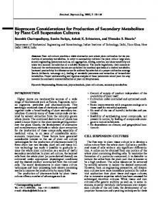
Table of Figures Figure 1. Product life-cycle showing key leverage points and major stakeholders...................... 11 Figure 2. Year to year change in apparent aluminum consumption in the US[6] ........................ 12 Figure 3. Year to year change in scrap generated in the US over the last two decades in thousands of metric tonnes[7]....................................................................................................... 12 Figure 4. Recent normalized London Metals Exchange daily cash settlement prices, Jan – Sept 2005 (Jan. 4, 2005 = 1) ................................................................................................................. 13 Figure 5. Scrap prices over two year period from multiple dealers[9] ......................................... 13 Figure 6. Compositional uncertainty (mean and standard deviation of various elements) in scrap aluminum siding sampled over the course of a year [4] ............................................................... 14 Figure 7. Schematic of scrap mixing illustrating shortcomings of mean based conventional method. Typical mean-based optimizations cannot differentiate between scrap A (small variance) and scrap B (large variance). ........................................................................................................ 18 Figure 8. Schematic comparing the conventional methods for representing scrap composition as a mean or as a compositional window. ......................................................................................... 19 Figure 9. Schematic of scrap mixing illustrating the conventional method of representing scrap as a compositional window; when the window is set to be one standard deviation from the mean, a significant amount of batch errors will still occur ........................................................................ 19 Figure 10. Scrap represented as compositional window combined with narrowed finished good specification targets: the window narrowing conventional method ............................................. 20 Figure 11. Discretely modeled probability distribution for compositional scenarios................... 25 Figure 12. Number of iterations to global or local optimum convergence for the chanceconstrained formulation (CC) and the penalty function formulation (Penalty) vs. the deterministic batch planning model (Det) with number of raw materials .......................................................... 34 Figure 13. Number of iterations to global or local optimum convergence for the chanceconstrained formulation (CC) and the penalty function formulation (Penalty) vs. the deterministic batch planning model (Det) with number of products .................................................................. 35 Figure 14. Number of iterations to global or local optimum convergence for the chanceconstrained formulation (CC) and the penalty function formulation (Penalty) vs. the deterministic batch planning model (Det) with number of compositions..................................... 35 Figure 15. Memory for the chance-constrained formulation (CC) and the penalty function formulation (Penalty) vs. the deterministic batch planning model (Det) with number of raw materials........................................................................................................................................ 36 Figure 16. Memory for the chance-constrained formulation (CC) and the penalty function formulation (Penalty) vs. the deterministic batch planning model (Det) with number of products ....................................................................................................................................................... 36 Figure 17. Memory for the chance-constrained formulation (CC) and the penalty function formulation (Penalty) vs. the deterministic batch planning model (Det) with number of compositions ................................................................................................................................. 36 Figure 18. Example Monte Carlo simulations of A) magnesium composition in alloy 390 and B) copper composition in alloy 380 for the base case chance constrained batch plan. Target alloy specifications are indicated by the bars; due to the high success rate specified by the α and β parameters, cases where the alloy is out of specification are infrequent. For all chance constrained cases, α was set to be 99.99% and β was set to be (1-α) or 0.01% unless otherwise indicated........................................................................................................................................ 40

7

Figure 19. Error rates and scrap use for the mean based method at various degrees of window narrowing. Over all conditions, the error rate is much higher than the chance-constrained method when the COV=50% ..................................................................................................................... 42 Figure 20. Error rates and scrap use for the mean based method at various degrees of window narrowing. At 75% window narrowing (25% original compositional window), the mean based method has equivalent scrap use to chance-constrained method but still a much higher error rate even with reduced variation (COV=20%) .................................................................................... 42 Figure 21. Comparison between base case results for chance-constrained and 30% window narrowing showing varying degrees of improved scrap consumption for the production of individual alloys (50% COV, 2 SD) ............................................................................................. 43 Figure 22. Comparison between base case results for chance-constrained and 30% window narrowing showing varying degrees of improved scrap consumption across scrap types. Scraps where the CC method finds usage opportunities are circled (50% COV, 2 SD) .......................... 43 Figure 23. Scrap usage and error rate of the chance-constrained method compared to varying window sizes for the window narrowing method. A window narrowing size of 30% (70% original composition window) was chosen for the base case due to nearly equivalent error rate with the chance constrained method ............................................................................................. 44 Figure 24. Scrap use and error rates for varying scrap compositional window representations for the window narrowing method (COV=50%, 30% WN). For a given variation in scrap composition, the finished good specification window size controls the error rate for this method. To maintain constant error rate, window size must be adjusted whenever scrap characteristics or availability change. ....................................................................................................................... 45 Figure 25. Scrap use and error rates for varying confidence intervals for the chance-constrained method. Error rate for the CC method is easily controlled through the alpha value specification and does not change significantly with scrap characteristics or availability. The base case alpha value of 99.90% gives a suitably low batch error rate.................................................................. 45 Figure 26. Improvement in scrap utilization of chance-constrained method over 30%, 20%, and 10% window narrowing methods (70%, 80%, and 90% windows) for a range of uncertainty conditions (SD=2) Base Case Comparison: COV=50%, 30% WN.............................................. 46 Figure 27. Improvement in production cost of chance-constrained method over 30%, 20%, and 10% window narrowing methods (70%, 80%, and 90% windows) for a range of uncertainty conditions (SD=2) Base Case Comparison: COV=50%, 30% WN.............................................. 47 Figure 28. Fluctuating error rates with increasing scrap variability at various window sizes for all variations of window narrowing method. CC method maintains consistent error rates. Base Case Comparison: COV=50%, 30% WN, SD=2.......................................................................... 47 Figure 29. Scrap usage comparison between chance-constrained method and conventional window narrowing with increasing scrap portfolio diversification, taking away in order of least used (30% WN, COV=20%, 50%, SD=2).................................................................................... 51 Figure 30. Error rate with increasing scrap diversification (COV=20% or 50%, SD=2, WN=70%) ....................................................................................................................................................... 51 Figure 31. Cost savings of chance-constrained method over conventional window narrowing method with increasing scrap portfolio diversification (COV=20% or 50%, SD=2, WN=70%) 52 Figure 32. Comparison of detailed scrap consumption of chance-constrained (CC) and window narrowing (WN) methods with increasing scrap type availability. While the number of scraps available for consumption increases from one to seven, the WN method continues to select only two scrap types. (COV=50%, SD=2, WN=80%) ......................................................................... 52

8

Figure 33. Comparing error rate for chance-constrained and window narrowing method for production of 100 kilotonne of 6061 alloy (COV=50%, 2 SD, WN=80%) ................................. 53 Figure 34. Comparison of stochastic Monte Carlo simulation of average copper composition for alloy 6061 produced according to production plans derived from either chance-constrained (CC) or window narrowing (WN) methods. .......................................................................................... 53 Figure 35. A) Comparison of individual scrap consumption when sampling from one or two piles of each scrap using the chance-constrained method B) Total effect of sampling diversification within the chance-constrained method (COV=50%).................................................................... 54 Figure 36. Percentages of old scrap consumed (total 1,154,000 metric tones) and distribution of end use shipments (total 9,699,000 metric tones) by category in the United States and Canada in 2005[95]........................................................................................................................................ 56 Figure 37. General scrap set consumption comparison for individual alloy sets, organized by series (CC Method, COV=50%, α=99.99%). ............................................................................... 60 Figure 38. Recycling friendly alloy set R (A) and market alloy (B) set M1 scrap use comparison for each different scrap “scenario” ............................................................................................... 61 Figure 39. Comparison of scrap used in the production portfolio of the 7XXX series alloys for each of the scrap scenarios............................................................................................................ 62 Figure 40. Comparison of scrap used in the production portfolio of the 5XXX series alloys for each of the scrap scenarios............................................................................................................ 63 Figure 41. Schematic representation of alloy compositional specification windows for the 4XXX and 5 XXX series alloys of all three sets ...................................................................................... 64 Figure 42. A) Improvement in potential scrap consumption from loosening Mg constraints on alloy 6063 from 10% to 95% of as-listed specification width (a given percentage on the x-axis translates into a Mg specification through the relationship εmax = εmin + x%(εmax-εmin), B) Effect on scrap consumption of overlaying a tightening of other constraints in conjunction with loosening the Mg constraint corresponding to the same value on the x-axis of the graph above (Figure 42A). The maximum specification of a given element on a specific plot follows, εmax = εmax - x%(εmax-εmin). The line marked A represents the effect of tightening all other specifications (Si, Fe, Cu, Mn, and Zn) in conjunction with a loosening of the Mg constraint of an equal percentage amount. ....................................................................................................................... 66 Figure 43. Framework to identify alloy modification targets and possible recycling-friendly alloys ............................................................................................................................................. 67 Figure 44. A) Improvement in scrap consumption of loosening Si constraints on alloy 3004, B) Effect on scrap consumption of now tightening other constraints in conjunction with loosening the Si constraint............................................................................................................................. 69 Figure 45. Product life-cycle showing key leverage points and major stakeholders.................... 73 Figure 46. Ellingham diagram for various reactions[105, 106].................................................... 74 Figure 47. Aluminum products in the United States by end use sector[7] ................................... 75 Figure 48. The cost and scrap utilization trade-offs of various strategies for dealing with compositional accumulation ......................................................................................................... 76

9

Table of Tables Table I. Projected scaling results for three stochastic methods (CC-chance constrained, Penpenalty function, and Rec- multi-stage recourse) compared to deterministic (Det) linear program for small scale case and typical production size case ................................................................... 31 Table II. Run parameters with varying number of raw materials (products=15 and compositions=10).......................................................................................................................... 32 Table III. Run parameters with varying number of raw materials (products=15 and compositions=10) for penalty function......................................................................................... 32 Table IV. Run parameters with varying number of products (raw materials=5 and compositions=10).......................................................................................................................... 33 Table V. Run parameters with varying number of products (raw materials=5 and compositions=10) for penalty function......................................................................................... 33 Table VI. Run parameters with varying number of compositions (raw materials=15 and products=15) ................................................................................................................................. 33 Table VII. Run parameters with varying number of compositions (raw materials=15 and products=15) for penalty function ................................................................................................ 33 Table VIII. Prices of Raw Materials ............................................................................................. 39 Table IX. Mean Compositions of Scrap Materials ....................................................................... 39 Table X. Finished Goods Chemical Specifications ...................................................................... 39 Table XI. Parameters for the base case analysis .......................................................................... 41 Table XII. Base case results showing mean based method and comparison of chance-constrained method versus 30% window narrowing (70% of original composition window) case at 2 standard deviations and COV=50% (kt = kilotonnes)................................................................................. 41 Table XIII. Base case results by alloy showing chance-constrained method versus 30% window narrowing case at 2 standard deviations and COV=50%. (MB = Mean Based, WN= Window narrowing, CC = Chance-Constrained) ........................................................................................ 41 Table XIV. Shadow Prices on Alloy Demand for Base Case comparing CC vs. WN ................. 48 Table XV. Shadow prices on binding compositional constraints for CC base case and WN base case (COV=50%, SD=2, window=70%). Values in parentheses are negative............................. 49 Table XVI. Average compositions for scrap sets and prices ........................................................ 56 Table XVII. Gross melt yield for scraps and primary .................................................................. 57 Table XVIII. Elemental yield ....................................................................................................... 58 Table XIX. Maximum and minimum compositional specifications for finished alloys in weight fraction[96] ................................................................................................................................... 58 Table XX. Baseline results showing comparison of scrap friendly alloys (Set R) with current alloys (Sets M1&M2) (CC Method, 50% COV, Total Production = 600 kt)............................... 59 Table XXI. Total scrap material usage for the varying scrap portfolios by alloy set. .................. 61 Table XXII. Scrap usage (in kilotons) for 7XXX series alloys ................................................... 62 Table XXIII. Scrap usage (in kilotons) for 5XXX series alloys.................................................. 63 Table XXIV. Compositional shadow prices for maximum specifications for 6XXX and 3XXX series market alloys....................................................................................................................... 66 Table XXV. Possible tramp elements that increase with recycling.............................................. 73

10

Chapter 1. Introduction One of the key engineering challenges of the 21st century will be reducing the harmful effects associated with a growing population and the attendant flows of materials[1, 2]. The materials community is uniquely positioned to play a central role in addressing these problems by fundamentally changing the materials and processes used by society. For this to happen, materials experts must begin to consider the environmental impacts of their design choices and will require additional analytical tools to quantify those broader implications. This thesis begins to address the need for these analytical tools for at least one element of a material’s environmental performance – the ability to be produced from secondary resources. Materials that perform well in this regard will be referred to herein as recycling-friendly. Within a materials’ life-cycle or production chain there are a variety of leverage points for increasing environmental performance (Figure 1). This work aims to improve materials decision making in two of these key areas: 1) blending decisions in manufacturing, and 2) alloy design decisions in product development. Usage Manufacture

Product Design & Development

Key Stakeholders Recovery & Firms Collection Producers OEM’s Recyclers Municipalities Secondary Consumers Markets Legislators Pre-Processing

Figure 1. Product life-cycle showing key leverage points and major stakeholders

1.1 Production uncertainties effecting blending decisions Uncertainty is a reality that confronts all businesses; materials producers are no exception. When business plans do not accommodate actual operating conditions, businesses are left with the negative economic impact of inefficient use of capital, materials, or potential market consumption. A significant set of economic disincentives emerge due to the various types of operational uncertainty that confront secondary metal processors [3-5]. In particular, depending on where one is in the production chain, business-critical sources of uncertainty include capricious demand, unstable availability of raw materials (particularly scrap materials), the precise composition of those raw materials, and the cost of factor inputs. An appreciation of these uncertainties can be gained by examining Figure 2 through Figure 5. Figure 2 shows the year to year change in aluminum apparent consumption in the United States over several decades, an illustration of the volatility of alloy demand. Scrap availability shows similar volatility (Figure 3), especially over the past few decades where much scrap has begun to be exported to rapidly industrializing countries such as China and Brazil.

11

Year to Year Change in Apparent Consumption (Mtonnes)

1.5 1 0.5 0 -0.5 -1 -1.5 1950

1960

1970

1980

1990

2000

Year to year change in scap availability (thousands tonnes)

Figure 2. Year to year change in apparent aluminum consumption in the US[6]

40 30 20 10 0 -101980

1985

1990

1995

2000

-20 -30

Figure 3. Year to year change in scrap generated in the US over the last two decades in thousands of metric tonnes[7]

Figure 4 shows the normalized London Metals Exchange price for primary aluminum over several months. Although the overall price trend of primary over a longer period (ie. the last four decades) is one which is clearly favorable to all aluminum producers, the significant variance of price represents not only a direct form of operating uncertainty, but also belies the underlying swings in demand which confront operational decision-makers. Scrap shows even larger volatility in price, due in part to geographic and regional price differences for different types of scrap materials. For example, scrap dealers near cities have larger supply of UBC’s (used beverage cans) and therefore can offer lower prices; large scrap dealers in the Midwest have access to large amounts of automotive-heavy mixed scraps and therefore lower prices on those types. Such large price differences (e.g. approximately 47% difference between the maximum and minimum prices for auto wheels) over such a short period of time (less than two years) can lead to significantly different blending decisions. All of these uncertainties have the largest adverse effect on those furthest from the customer, e.g. materials producers, due to the feedback mechanisms inherent to typical market-based supply-chains [8]. Nevertheless, despite real uncertainties, definite business-critical decisions must be made on a daily basis.

12

Normalized Price

1.2

1.1

1

0.9

0.8 Jan-05

Mar-05

May-05

Jul-05

Sep-05

Figure 4. Recent normalized London Metals Exchange daily cash settlement prices, Jan – Sept 2005 (Jan. 4, 2005 = 1)

Scrap Prices ($/lb.)

$1.4

Cast Aluminum Shredded UBC

Auto Wheels Remelt Ingot

Nodules

$1.2 $1.0 $0.8 $0.6 $0.4 Jan-07

Apr-07

Aug-07 Nov-07 Feb-08

Jun-08 Sep-08

Figure 5. Scrap prices over two year period from multiple dealers[9]

Previous work has shown that explicit consideration of operational uncertainties (i.e., through the use of stochastic programming), in production planning can improve batch operator decisions both in terms of reduced operating costs and increased scrap consumption [10-15]. Such results are consistent with improvements observed in other contexts [16-21]. This thesis introduces the use of a related framework – referred to as stochastic programming – to explicitly address a previously unexplored source of uncertainty that confounds secondary batch planning – compositional variation of secondary raw materials. Elemental considerations for scrap have been identified as the most significant source of uncertainty in the production process [5, 22]. To provide an indication of the scope of this form of uncertainty, Figure 6 shows composition and standard deviation of recycled aluminum siding sampled over a period of a year; one can see the wide range in both mean and variance. Considering the many types of recycled materials secondary producers utilize multiplied by the dozens of relevant compositional elements, it is clear that compositional uncertainty makes it difficult to meet quality specifications and, thereby, creates a strong disincentive to use.

13

The stochastic optimization methods that will be presented attempt to address this problem by modifying conventional methods of dealing with compositional uncertainty. These conventional methods are deterministic or static in nature. A comparison of stochastic and conventional methods will be made in regards to both their scrap use and operational economics; these are examined through case studies and targeted simulations. 1.6% Weight Percent

1.4% 1.2%

95%

Coefficient of Variation = 55% 256% 121% 2639% 3134%

1.0% 0.8% Fe

0.6%

Mn

0.4% 0.2%

Si

Cu Mg

0.0%

Zn

Compositional Elements Figure 6. Compositional uncertainty (mean and standard deviation of various elements) in scrap aluminum siding sampled over the course of a year [4]

1.2 Recycling friendly alloy design How to design alloys that are more recycling friendly or, in other words, more able to accommodate scrap materials in their production portfolios, is a challenging question. Industry experts and literature have provided a variety of suggestions. A much discussed strategy involves the development of single alloys that could meet the performance requirements currently filled by multiple alloys. For example, an alloy that could replace both 5XXX and 6XXX materials in transportation applications[23, 24]. Some even propose legislation or regulations to limit the number of alloys that can be used in certain products such as cars or aircraft[25]. Other suggestions involve modifying the forming and joining of aluminum, for example, replacing conventional welding with mechanical joining, laser welding, or friction stir welding[26]. Specific suggestions concerning the modifications of alloys include higher maximum compositional specifications for certain elements that will not adversely affect alloy properties, wider specification targets (i.e. higher maximums and lower minimums), or translating compositional constraints to specifications based on performance[27, 28]. However, no quantitative assessments of the efficacy of these suggestions on the ability of a recycler or recycling system to use more secondary raw materials have been reported in the literature. Furthermore, no methodology has been discussed that would quantitatively assess in what context these strategies should be applied. Despite these specific issues, a range of literature has examined the use of decision-analysis models to improve the economic and resource use performance of recycling operations. The most pertinent include those that apply a range of mathematical programming techniques to improve decisions about raw materials purchasing strategy, technology selection[19, 29, 30], and the application of upgrading and sorting for secondary raw materials[31, 32]. Although 14

notionally these models can be used iteratively to evaluate how some change would affect the ability to use secondary raw materials, none are applicable to evaluating the design of multispecification alloys. The primary challenge of evaluating the recycling-friendliness of multi-specification alloys is that it is a context dependent property; how much scrap an alloy can accommodate will be based on not only the compositional characteristics of the alloy itself, but also the types of scraps available to producers, the compositional characteristics of those scraps, and their metallic yield. As a result, a method to evaluate recycling-friendliness must be able to account for the confluence of these detailed effects. Two sets of previous work on decision-analysis models have been specifically applied to recycling performance of secondary aluminum production and form the basis for addressing this need. The first set of studies by Reuter, van Schaik, and others[19, 29-31, 33-35] utilized optimization methods and dynamic modeling to optimize the recycling system for end-of-life vehicles, including the light-metals within them. This work and the models it presents can be used to guide operational and technological decisions by recyclers and to provide reasonable recovery expectations for recyclers, and more broadly, policy-makers. The second set is previous work by the author [36] and Rong[5] which describes schematic, mathematical programming models that identify the optimal raw materials mix to blend to produce a given multispecification alloy or alloy production portfolio. These models are extensions of batch planning models that have been developed for decades and are available and used within the secondary metals industry today. To date, such models have been used to evaluate the effectiveness of improved operational practices and alloy substitution to increase potential scrap use. In previous work, it was hypothesized that model-derived sensitivity analysis information could be used to direct alloy design and demonstrated that, for a stylized case, such sensitivity analysis information varied significantly across specification and alloy. This thesis extends this previous work by a) characterizing the challenge of developing recycling-friendly alloys due to the contextual sensitivity of that property; b) demonstrating how such decision-support models can be used to evaluate post-facto the potential scrap usage of alloys across a range of raw materials contexts; and (c) exploring the value of sensitivity analysis information to proactively identify the most effective alloy modification strategies that can drive increased potential scrap use. With regard to the latter, this thesis extends previous discussions by exploring in detail how sensitivity analysis information actually correlates with potential scrap use performance and how both the sensitivity analysis information and the associated potential scrap use effect changes with individual and coordinated specification modifications. In exploring the latter for two distinct cases, this thesis suggests that real potential exists for increasing potential scrap use through alloy redesign while remaining within established compositional specifications. Finally, this thesis extends previous work in this space by presenting a schematic algorithm for explicitly incorporating uncertain metal yield into the analyses of alloy design specifically, and recycler operational decisions more broadly. Both the model and cases discussed herein are intended to be schematic in nature. Much work still remains to capture the metallurgical complexity of the recycling process; nevertheless, the results presented show that this framework holds promise to be a valuable tool in the

15

metallurgists toolkit. Furthermore, a recycling evaluation tool, irrespective of scope or fidelity, would always be but a single element in the overall alloy design process. Traditional and emerging metallurgical methods will be required to identify alloys capable of meeting demanding physical performance requirements. Nevertheless, efficient design of resourceconscious materials depends upon analytical tools capable of projecting the impact of design choices on recycling performance.

16

Chapter 2. Batch planning models 2.1 Linear optimization A large variety of modeling tools are available to help support the decisions of batch planners; many producers make use of linear optimization techniques [29]. Blending problems have been addressed with linear programming models for decades[37]. These models can improve decisions about raw materials purchasing and mixing as well as the upgrading and sorting of secondary materials [11, 19, 30]. Additionally, linear optimization techniques have been implemented to address larger scale aluminum recycling questions as well. Studies by [33-35, 39] have utilized dynamic modeling and large datasets to calculate optimized recovery rates for end-of-life vehicles in order to guide operational and technological decisions by recyclers and to provide reasonable recovery expectations for recyclers, and more broadly, legislators. Analytical approaches may be used within such optimization tools to embed consideration of uncertainty in the decision-making, but generally this occurs through the use of statistical analyses that are used to forecast expected outcomes. Although this combination of statistical analysis and modeling can be powerful, it suffers from two fundamental limitations. First of all, implicit assessments based on mean expected conditions assume that deviation from that value has symmetric consequences. For many production related decisions within the cast-house, the repercussion of missing a forecast are inherently non-symmetrical. Additionally, deterministic approaches generally do not provide proactive mechanisms to modify production strategies as prevailing conditions evolve. 2.2 Modifying deterministic batch planning models 2.2.1 Mean based conventional method Before exploring more advanced blending models, it is first helpful to understand how raw material compositional variation is handled presently within many batch planning tools. Although it is well known that most scraps will have some sort of compositional distribution, producers tend to model raw materials using their mean or expected value (Ai) or some other measure derived from these (e.g., mean + 10%). The goal of batch operators is then to combine these raw materials in such a way that the composition of finished goods falls within desired maximum and minimum targets. This can be stated mathematically by the following: max A min Bf f B f ≤ ∑ Ai x i ≤ A f

(1)

i

where the symbol A represents the amount, expressed as a mass fraction, of a certain element such as silicon, magnesium, zinc, etc. that is either contained within a raw material, i, or cannot be exceeded / fallen below within a finished alloy, f. It is important to note that the minimum and maximum Af are specifications while Ai is the actual composition. B is the amount of finished product f produced, while x is the amount of raw material used in the production of f. For clarity, the yield of A from raw material into finished alloy has been assumed to be one but could be changed to represent actual yields. Producing within specification based on the initial furnace charge is a key business objective of cast-shop operators [5]. Missed specifications require rework in the form of compositional additions or, even worse, dilution. Such rework is costly because it increases consumption of primary raw materials, energy, and time.

17

This method of representing recycled materials solely by their mean has one major shortcoming: it cannot differentiate between two scraps with the same mean but different variances. To illustrate this shortcoming, imagine a finished alloy is going to be made of only one raw material and can select between recycled materials: Scrap A or Scrap B. Considering only one compositional alloying element, (silicon, for example), assume both scraps have the same mean but scrap B has a larger standard deviation (variability). If these scraps have high silicon levels, they will be combined with primary raw materials until their mean composition is diluted inside the finished good’s target minimum (Figure 7). Three pricing scenarios can be imagined. If scrap A were less expensive than scrap B, the model would choose all scrap A; this is highly unlikely. If scrap B is less expensive than scrap A as would be expected due to its higher level of compositional uncertainty, the mean based model would choose all scrap B. This would result in a finished good with a high likelihood of being out of specification. If the two scraps were equal in price, the mean based model would choose between the two indifferently which is also not optimal. Additionally, as will be shown subsequently, it is difficult to guarantee reasonable error rates at mid to high levels of compositional variation for mean-based methods.

Specification Target Scrap Mean

A:

Out of Spec Scrap Variance

B:

Dilution In Spec

More Batch Errors

Variance B > Variance A

Composition: X wt%

Figure 7. Schematic of scrap mixing illustrating shortcomings of mean based conventional method. Typical mean-based optimizations cannot differentiate between scrap A (small variance) and scrap B (large variance).

2.2.2 Compositional window conventional method To address this shortcoming, some producers model scrap composition as a range or window. In this method, the width of the window (i.e., the modeled maximum and minimum compositional limits for the scrap) is set based on the scrap’s mean and variance. These maximum and minimum limits are then compared to the maximum and minimum specifications of the finished goods to establish batch plans. This method for representing scrap composition is compared schematically to the mean based method in Figure 8. Using this scrap compositional window method, batch planning models seek out combinations of raw materials such that recycled materials are combined with primary metal until the minimum composition limit of the mixture is inside the finished good’s target minimum and / or the maximum limit is inside of the maximum specification. The scrap compositional window method has advantages over the mean based method in that it can differentiate between scraps with the same mean but different 18

variances and will provide a much lower error rate for being within specification, especially as scrap becomes more variable. However, shortcomings still exist; Figure 9 shows that when the compositional window is set at one standard deviation (σ) from the mean, a significant number of batch errors can still occur. Compositional Window

Mean Based

Figure 8. Schematic comparing the conventional methods for representing scrap composition as a mean or as a compositional window.

Specification Target Scrap Mean

Dilution

Scrap Variance

Comp Window

Batch Error

Composition: X wt%

Figure 9. Schematic of scrap mixing illustrating the conventional method of representing scrap as a compositional window; when the window is set to be one standard deviation from the mean, a significant amount of batch errors will still occur

2.2.3 Window narrowing of finished good specifications To further limit the incidence of rework, operators often modify the mean based or compositional window methods by generating batch plans based on more narrow finished goods specification targets[40]. This narrowing of the target window creates a margin of safety around compositional specifications such that a high level of likelihood is maintained for the finished goods compositions to fall within their actual specifications, shown schematically in Figure 10. This percentage of the original finished good specification is then used as the sole adjustment for dealing with uncertainty.

19

This practice modifies the constraint expressed in Equation (1) as shown in Equations (2) and (3) in which F is defined to be an adjustment factor of the specification range. The combination of representing scrap as a composition window and using a narrowed finished good specification window is the most robust conventional method for modeling scrap mixing decision and will be used as a conventional base case and referred to as the window narrowing (WN) method throughout the balance of this document.

∑ i

∑ i

∑ i

(1 − F ) m ax Af B f 2 (1 + F ) m in Aim in x i ≥ Af B f 2

⎫ ⎪⎪ ⎬ ⎪ ⎪⎭ Aim ax x i ≤ (1 − F ) A mf ax B f ⎫ ⎪ ⎬ m in m in ∑i Ai x i ≥ A f B f ⎪⎭

Aim ax x i ≤

, A mf in > 0

(2)

, A mf in = 0

(3)

Specification Target

Dilution Comp Window

Narrowed Target

Very Low or No Error

Composition: X wt% Figure 10. Scrap represented as compositional window combined with narrowed finished good specification targets: the window narrowing conventional method

2.3 Shortcomings of conventional methods Although window narrowing does offer a mechanism to control the risk of errant production, various issues arise with this practice. Generally, the window narrowing method is the most conservative method for a given error rate, or number of batches that fall outside of the finished goods specifications. Other prevalent methods presented in the literature also aim to maintain a linear performance constraint while considering variability in scrap composition[41, 42]. Work done by Debeau[43] in the steel industry cautions that simply using linear programming for batch planning problems is not sufficient and suggests additional constraints to deal with variable raw materials. While in the same way as window narrowing these methods help to decrease the probability of batches being out of specification, they all share the trait of insufficient accounting for the impact on variance when combining scraps.

20

To illustrate this shortcoming, imagine a finished alloy is going to be made of only two raw materials: Scrap A and B. Considering only one compositional alloying element, (silicon, for example), Equation (4) shows the expected outcome of combining a kilograms of Scrap A and b kilograms of Scrap B from the perspective of the window in window method. The mean and variance of the combination is assumed to be simply the weighted sum of the individual pile’s mean and variance. For example, combining 2 kilograms of Scrap A (µ=10% silicon σ=5%) and 2 kilograms of Scrap B (µ=10% silicon σ=5%) will result in a combination with µ= 2 kg*10% + 2 kg*10% = 40%/ 4 kg = 10% silicon and σ= 2kg*5% + 2kg*5% = 20%/4kg = 5%. In summary, the variance of the composition of a finished alloy will increase linearly as scrap piles are combined. µ A+ B = aµ A + bµ B (4) σ A+ B = aσ A + bσ B However, fundamental statistics shows that the combined scrap will have actual mean and variance according to Equation (5)[44]. So taking the example above (2 kilograms from each scrap pile) will result in the same mean as calculated above but the variance will be much different. In a case where the scrap pile compositions are completely uncorrelated, the variance will be σ= ((2kg)2*(5%)2 + (2kg)2*(5%)2)1/2= 14%/4kg = 3.5%. In reality, some correlations between scrap pile compositions would be expected and for these cases, the variance would be slightly higher than the example given, however, never as high as the weighted sum. So for all realistic cases, the variance of the composition of a finished alloy will increase sub-linearly as scrap piles are combined. The conservative nature of the window narrowing method is a direct consequence of its overestimation of compositional variance.

µ A+ B = aµ A + bµ B σ A+ B = a 2σ A2 + b 2σ B2 + 2ab cov( A, B)

(5)

Another shortcoming of conventional window narrowing is that it may be difficult to determine the necessary amount of narrowing and therefore over-compensation can often occur. Tightening the window too much could cause the system to under utilize available secondary materials. Not meeting the finished good compositional specifications is an even larger problem that results in rework requiring time, energy, and money. An implied margin of error will exist depending on the size of the window; however, the static nature of the method does not provide an intrinsic method to tailor practices to these different error rates and therefore may penalize the system’s ability to utilize scrap efficiently. For example, referring back to Figure 7, implementing the same window narrowing strategy for both scraps would result in under utilizing Scrap A and having high error rate when using Scrap B. For the operator tracking the compositional distribution of incoming raw materials, a mean based method would be more sensitive to these changes. Relating the margin of error to the underlying uncertainty in the chemical compositions of the raw materials may be a better practice and thereby provide both increased scrap consumption and associated economic benefits. The following section describes a method which provides just this capability.

21

Chapter 3. Methods 3.1 Stochastic programming Stochastic programming techniques encompass a large set of problems that deal with uncertainty of one form or another in the formulation. Often, this is accomplished by considering some form of probability and/or statistics within the objective function or constraints. Pioneers in the field have done work in an extremely wide range of applications including: agricultural applications including farm management[45, 46] and irrigation, economics[47, 48], finance[49, 50], assignment [51], facility location[52], inventory, water storage and reservoir management, energy, and production. Stochastic programs have been in use for solving product mix and blending problems for decades as well. Particular applications include nutrient blending for crops[53], humans[54], and livestock[55, 56], product mix[57], coal blending[58], asphalt mixing[59], fertilizer mixing at a chemical plant[60], and most prevalent, petrochemicals including gasoline[61]. Methods in stochastic programming are generally divided into two broad categories: single stage and multi-stage stochastic programs[62]. This work will explore the use of a multi-stage recourse problem for dealing with compositional uncertainty as well as two single stage methods: the use of a penalty within the objective function and the use of chanceconstraints within the compositional constraints. The computational complexity and scaling of these three stochastic methods compared to deterministic linear programming methods will be the metrics used to select an appropriate method for managing raw material uncertainty in metals blending problems (Section 4). 3.1.1 Multi-stage recourse stochastic programs A recourse model consists of multi-stage decisions that must be made prior to an uncertain event. The associated consequence or recourse is a second stage reaction that depends on the decision made at the first stage and the outcome of the uncertain event, shown schematically in Figure 3. Recourse models have a wide range of applications including product planning[63], transportation networks[64], energy and electricity networks[42, 65], supply chain, inventory, and manufacturing networks[66-68], finance[69], and human resource planning[70]. The objective function for a recourse problem, which is to be either minimized or maximized, can be mathematically stated as follows:

f (C , X 1 ) + g ( C , p , X 2 )

(6)

In Eq (6), the contribution from stage one to the objective function is given by the function f(.). X1 is the vector of decision variables from stage one. The contribution from stage two to the objective function is given by the function g(.). X2 is the vector of stage-two recourse variables over all possible uncertain outcomes and p is the vector of the probabilities of those outcomes. The overall cost of the recourse decisions to the overall objective is weighted by those probabilities. Therefore, the objective is an expected average objective rather than a deterministic objective. C is the cost vector whose aggregate contribution to the objective function is being maximized or minimized in this optimization problem.

22

A Priori Decision: Lower Cost Matls

Uncertainty Outcome: Scrap Composition

Recourse Decisions: Higher Cost Matls

= Outcome Node = Decision Node

Time

Figure 3. Schematic representation of recourse model The variables to solve for are X1i, X1ijz and X2ijz which are translated into the recourse batch planning optimization model together with other notations used in the problem formulation (Eq (7) to (13)). Min:

∑C

i

i

X i1 + ∑ Crework Pz X ijz2 − ∑ SCi Pz Riz r, j,z

∀i

s.t.:

(7)

i,z

X i1 ≤ Ai

(8)

The amount of residual raw materials for each scenario is calculated as: 1 ∀i , z Riz = X i1 − ∑ X ijz

(9)

j

For each compositional scenario z there are supply constraints as determined by the amount of raw materials pre-purchased,

∑X

∀i , z

1 ijz

≤ X i1

j

(10)

Eq (10) enforces the aforementioned condition that raw materials at the reduced cost (Ci) must be ordered before final production. As such, at production time, a cost of rework (Crework, where Crework >> Ci) must be assessed for all raw materials purchased in the second stage decision. Similarly, a production constraint exists for each scenario, quantifying how much of each alloy must be produced:

∀j

∑X i

1 ijz

+ ∑ X ijz2 = B jz ≥ M jz i

(11)

23

For each alloying element k, the composition of each alloy produced must meet production specifications [28]:

∀ j ,k

∑x ε

1 ij ik

i

∀ j ,k

+ ∑ xij2ε ik ≤ B j ε max jk

∑x ε

1 ij ik

i

(12)

i

+ ∑ xij2ε ik ≥ B j ε min jk i

(13)

All other variables are defined below: Ci = unit cost ($/T) of raw material i Ai = mass of raw material i available for purchasing ε ik = average mass element k in raw material i Mj = mass of finished good j demanded Bj = mass of finished good j produced εmaxjk = max. mass element k in finished good j εminjk = min. mass element k in finished good j Rsz = Residual amount of raw material i unused in scenario z D = 1 – discount on the value of unused scrap materials Pz = probability of occurrence for compositional scenario z xijz = amount of raw material i to be acquired on demand for the production of finished good j under demand scenario z Ai = amount of raw material i available for pre-purchasing In the notation of Eq (6), the objective function can be decomposed into two parts:

f (C , X 1 ) = ∑ Ci X i1 i

g (C , p, X 2 ) = ∑ Crework Pz X ijz2 − ∑ SCi Pz Riz i, j,z

(14) (15)

i,z

The stage one component, Eq (14), consists of only cost contributions from the raw materials purchased initially at a lower cost. The stage two cost components, Eq (15), consist of the effects of additional higher priced raw material purchased, the additional cost of having to fix batches that are out of specification, and the salvage value of unused raw materials. It is prohibitively computationally expensive to include a continuous distribution for the compositional scenarios. Therefore, each scenario is represented discretely with some associated probability (Figure 11). the problem will then scale with the number of discrete compositions used to represent some variance around the mean composition, this will be explored more fully in Chapter 4.

24

35% Probability (%)

30% 25% 20% 15% 10% 5% 0% 2σ

1σ

µ

1σ

2σ

Figure 11. Discretely modeled probability distribution for compositional scenarios

3.1.2 Chance-constrained stochastic programming Stochastic programming methods including chance-constrained variants were first formulated by Charnes and Cooper [71, 72] as mechanisms to embed a more rich set of statistical information into optimization based decision models. This technique is often used when the consequences for not meeting certain constraints are unknown. Typical applications include feed mixing[55, 56], reservoir management[73], nutritional planning, inventory control, metals blending[32, 74], scheduling problems[75], and water quality. Miller and Wagner [76] were the first to apply joint probabilistic constraints, however, could only consider independent random variables on one side of the equation, not simultaneously. These mathematical techniques became more useful for real world sized problems in the 1970’s, when computational power was beginning to grow rapidly. Prekopa [77] introduced stochastic constraints as they are used currently: stochastically dependent joint probabilistic constraints. An excellent review of stochastic programming including the use of joint chance-constraints can be found in [78] while a variety of recent numerical applications are available [19, 73, 79]. In the context of cast-shop batch planning, the chance-constrained method allows the compositional constraints to be modified such that 1) the model embeds knowledge of both the mean and variance of available raw materials and 2) the user can query the model for optimal solutions which provide a specified level of confidence for meeting the compositional specifications. This method relates the desired level of confidence to the underlying standard deviations observed in the sampled raw materials. With the understanding that the compositional constraints will not always be satisfied due to inherent uncertainty, they can be rewritten as probabilistic expressions and transformed into their deterministic equivalents. For the problem at hand, the constraints expressed in Equations (2) and (3) are transformed into Equations (16) and (17): ⎧ ⎫ Pr ⎨∑ Ai xi ≤ F fmax A max Bf ⎬ ≥ α (16) f ⎩ i ⎭ → ∑ Ai xi + X (α )(∑∑ ρ ij σ iσ j xi x j )1 / 2 ≤ F fmax A max Bf f i

i

j

25

⎧ ⎫ Pr ⎨∑ Ai xi ≥ F fmin A min (17) f Bf ⎬ ≥ β ⎩ i ⎭ → ∑ Ai xi + X (1 − β )(∑ ∑ ρ ij σ iσ j xi x j )1 / 2 ≥ F fmin A min Bf f i

i

j

The statements Pr(.) state that those constraints which were originally required to be strictly satisfied are now only satisfied α and β percent of the time. Thus α and β are desired levels of confidence factors which the operator can use to adjust his or her sense of importance for that particular elemental composition to be within specifications. The function X(.) is the inverse of a normalized cumulative Gaussian distribution function1 which relates the underlying raw material composition standard deviations to the desired level of confidence. Work by Peterson[4] on scrap variability has shown this estimation to be applicable in many cases. The symbol ρij represents the correlation between the fluctuations in composition of raw material i and j. By definition ρij = 1 when i = j. The chance-constrained problem can be formulated as follows in Equations (18) through (22) as a linear optimization model. The goal of this model is to identify the production plan, referred to subsequently as a batch plan, that will minimize the overall expected production costs (C(x)) of meeting finished good compositional specifications through optimal and efficient use of primary and secondary raw materials (Eq.(18)). To more accurately capture the behavior of a recycling operation, this simple objective is subject to a number of specific constraints. Firstly, raw materials cannot be prescribed in the batch plan in excess of the quantity available (Eq.(19)). Secondly, the batch plan must lead to production quantities that meet or exceed the established target for each alloy (Eq.(20)). Finally, the likelihood that a batch plan produces alloys within compositional specifications must exceed a specified probability (Eqs. (21) and (22)). This is accomplished by relating the likelihood of achieving a certain finished alloy composition to the underlying statistical characteristics of the raw material compositions (i.e., εik,,σ(ε)ik, and ρ(ε)ilk) and the desired confidence limits, as established by the parameters α and β. With the understanding that the compositional constraints will not always be satisfied due to inherent uncertainty, they can be rewritten as probabilistic expressions and transformed into their deterministic equivalents. (18) Min: ∑ Ci X i i

∀i

Subject to:

∑x

ij

= X i ≤ Ai

(19)

∑x

ij

= Bj ≥ M j

(20)

j

∀j

i

∀ j ,k

∑ x ε + X (α )(∑∑ ρ ε σ ε σ ε x x ) ≤ B ε ∑ x ε + X (1 − β )(∑∑ ρ ε σ ε σ ε x x ) ≥ B ε 1/2

i

∀ j ,k

( ) ilk

ij ik

i

( ) ik

( ) lk ijk ljk

j

max jk

1/2

( ) ilk

ij ik

i

(21)

l

i

( ) ik

( ) lk ijk ljk

j

min jk

(22)

l

All other variables are defined below: Ci = unit cost ($/T) of raw material i xij = mass of raw material i used in making finished good j Xi = mass (kt) purchased raw material i (both primary and scrap) Ai = mass of raw material i available for purchasing 1

Other statistical distributions can also be assumed.

26

ε ik = average mass element k in raw material i σ(ε)ik = standard deviation of the composition (ε) of element k in raw material i ρ(ε)ilk = correlation coefficient between composition (ε) of element k in raw materials i and l (ρil = 1 when i=l) Bj = mass of finished good j produced Mj = mass of finished good j demanded εmaxjk = max. mass element k in finished good j εminjk = min. mass element k in finished good j Χ (_) = inverse of a normalized cumulative Gaussian distribution function α = likelihood that the actual composition will fall below the upper limit of final alloy composition β = likelihood that the actual composition will fall above the lower limit of final alloy composition Of these, the ones that may require further clarification are α, β, and X(). Individually, α and β represent the likelihood that the batch plan identified by the model will result in a composition that is lower than the upper compositional limit and greater than the lower compositional limit, respectively. X(), the inverse normalized cumulative Gaussian distribution function, characterizes the relative distance from the mean that corresponds to the designated level of likelihood. 3.1.3 Penalty functions Another stochastic programming method described in the literature [80-82] is the use of a penalty function added to the least cost objective function. While the majority of the applications are for blending within the chemicals industry, their extension to metals batch mixing is quite straightforward as formulated in Eq.(23) through (27). Typically these models multiply some cost of rework (Crework) with the probability of being out of specification. The objective function then becomes: ⎡ ⎧ ⎫ ⎧ min ⎫ ⎤ ∑i Ci X i + Crework * ⎢∀ j ,k Pr ⎩⎨∑i xijε ik ≤ B jε max jk ⎬ ∀ j , k + Pr ⎨∑ xij ε ik ≥ B j ε jk ⎬ ⎥ ⎭ ⎩ i ⎭⎦ (23) ⎣ Min.: This causes the problem to have nonlinearities in the objective function; each of the constraints will be unchanged from the deterministic formulations and therefore will remain linear as shown below. (24) Subject to: ∀i ∑ xij = X i ≤ Ai j

∀j

∑x = B ≥ M ∑x ε ≤ B ε ij

j

(25)

max jk

(26)

≥ B j ε min jk

(27)

j

i

∀ j ,k

ij ik

j

i

∀ j ,k

∑x ε

ij ik

i

3.2 Addition of stochastic yield to chance-constrained formulation

To make the chance-constrained formulation more flexible to capture the metallurgical complexity of modern recycling processes it can be amended to comprehend the effects of

27

material yield. To increase the precision of the model and to accommodate current data collection practices within industry, yield is represented by two parameters: elemental yield and gross yield. The elemental yield, Yik , represents the fractional increase or decrease of the mass of alloying element k in the melt derived from incoming material inflow i. The mechanisms that drive such mass change vary widely by element. For example, iron is expected to increase due to pick-up from processing equipment and silicon will increase due to pick-up from the furnace refractories. Other elements may decrease due to oxide formation (zinc and magnesium may form spinel), volatization, or sinking/settling of the melt. The second parameter used to capture the effects of yield is the gross melt yield, Gi, which represents total metal loss (i.e. aluminum and other elements) as a fraction of incoming raw materials i. Such loss occurs due to dross formation, spills, etc. Notably, both forms of yield are expected to exhibit some variation from batch to batch. As such, they will be incorporated into the model as stochastic parameters. It is important to point out that while this treatment of yield does significantly increase the flexibility and the potential fidelity of the model framework, it does not capture all possible effects. In contexts where elemental interaction is larger than the natural stochastic variation of the yield, additional second order terms would need to be incorporated. Similarly, works by van Schaik and Reuter[83] [84, 85] have shown that particle size distribution and scrap conformation are key factors in metal yield and, therefore, operational decisions. The formulation presented herein does not address such effects directly. For business critical decisions where the operational decisions will affect the yield variation associated with particle size, analysts should carefully consider the explicit treatment of these issues for their specific context. It is important to note, however, that irrespective of the form of the performance function (i.e. the left-hand sides of Equations (21) and (22) which relate the composition of the incoming raw materials to the composition of the outgoing finished alloy) most modern optimization packages can generate shadow price information on the constraint. As such, the types of work demonstrated herein should be extensible even to other blending models. If the metallurgical yield is in fact stochastic in nature, its effect cannot be accounted for with a scalar transformation of the above formulation. Instead, the constraints on production quantity (Eq.(20)) and composition (Eqs.(21) and (22)) must be redeveloped. The probabilistic constraints incorporating yield can be expressed as: ⎧ ⎫ (28) ∀ j Pr ⎨ B 'j = ∑ xij Gi ≤ M j ⎬ ≥ γ i ⎩ ⎭ ⎧ ⎫ ' (29) ∀ j , k Pr ⎨a jk = ∑Yik ε ik xij ≤ B'jε max jk ⎬ ≥ α i ⎩ ⎭ ⎧ ⎫ ' (30) ∀ j , k Pr ⎨a jk = ∑Yik ε ik xij ≥ B'jε min jk ⎬ ≥ β i ⎩ ⎭ where Yik and Gi are random variables as defined above, εik is a random variable representing the actual amount of k in raw material i, B 'j is the actual quantity of batch j produced, ajk is the actual quantity of element k in finished batch j, and γ, α’ and β’ are the minimum acceptable likelihood of the respective conditions being true.

28

The former (Eq.(28)) can be transformed directly into its deterministic equivalent as follows:

∑ x G + Χ(γ ) ∑∑ ρ

∀j

ij

i

i

i

( G ) il

σ (G )iσ (G )l xij xlj ≤ M j

(31)

l

Realizing the same for the new compositional constraint requires additional manipulation. First, it is helpful to replace the product of the two random variables Yik ε ik with Ψik which is also a random variable. Formally, the distribution of Ψik is a modified Bessel function of the second kind [27]. However, for typical characteristics of elemental yield and elemental content, Ψik can be well approximated with a normal distribution such that:

Ψ ik ≅ Yik ε ik and Ψ ik ~ N (Ψ ik , σ (2Ψ )ik ) where Ψik = Yik ε ik and σ

2 ( Ψ ) ik

=ε σ 2 ik

2 (Y ) i

+Y σ 2 ik

2 (ε ) ik

+σ

σ

2 (Y ) i

2 (ε )ik

[84, 85]

(32) (33)

Incorporating these relationships into and rearranging Eq (29) yields the following probabilistic constraint: ⎧ ⎫ ' (34) ∀ j , k Pr ⎨∑ ( Ψ ik − Giε max jk ) xij ≤ 0 ⎬ ≥ α ⎩ i ⎭ Again, to simplify, it is helpful to define a new variable, φijkmax , such that:

∀i , j ,k

φijkmax ≡ Ψ ik − Giε max jk

2 max 2 2 where φijkmax = Ψ ik − Giε max jk and σ (φ ) ijk = σ ( Ψ ) ik + (ε jk ) σ ( G ) i

(35) (36)

Using these definitions it is possible to convert the probabilistic constraint Eq.(34) into its deterministic equivalent of the form:

∑φ

∀ j ,k

x + X (α ' )

max ijk ij

i

∑∑ ρ φ

σ (φ )ijkσ (φ )ljk xij xlj ≤ 0

( ) ilk

i

(37)

l

Using an identical approach it is possible to develop Eq. (37) into an analogous constraint on minimum compositional specifications of the form:

∀ j ,k

∑φ

x + X (1 − β ' )

min ijk ij

i

∑∑ ρ φ

σ (φ )ijkσ (φ )ljk xij xlj ≤ 0

( ) ilk

i

(38)

l

where φijkmin ≡ Ψ ik − Giε min jk

(39)

Replacing equations (20), (21), and (22) with their analogs (31), (37), and (38), respectively, creates a schematic model that explicitly addresses uncertainty in both raw materials composition and yield.

29

3.3 Monte Carlo simulations

To test the optimal batch solutions given by both the deterministic and stochastic methods, Monte Carlo simulations were run to evaluate the robustness of batch plans to variation in the composition of incoming scrap materials. The Monte Carlo method uses pseudo-random numbers (i.e. not truly random in the sense that they are generated by numerical algorithms) to statistically simulate random variables, in this case, scrap composition.

30

Chapter 4. Computational complexity and scaling 4.1 Projected scaling

The formulations of the stochastic methods (recourse, penalty function, and chance-constrained) as coded in Lingo by Lindo Systems are listed in Appendix A. The deterministic formulation has been omitted due to its simplicity. The three main inputs that scale the size of the batch mixing problem are the number of products j (alloys in this case study), number of raw materials i (this includes scrap, primary aluminum, and alloying elements), and the number of compositions k being tracked (elements such as Si, Mg, etc.). For this scaling analysis, the chance constrained formulation without yield as an addition (see Eq. through ) was compared to a deterministic linear programming batch plan. The addition of yield to the model does not significantly change these results as the yield terms are absorbed into the stochastic composition number. The recourse and penalty function stochastic methods are also presented. The effect of these input parameters is presented for the number of iterations required for convergence (either to global or local optimum) as well as storage, which would be of interest to users of these optimization techniques. For the deterministic method the total number of decision variables will be i x j (O(mn)) and the total number of constraints will be i (availability of raw materials) + j (batch size constraints) + 2 x j x k (compositional constraints); this will be dominated by the compositional terms and therefore will be O(2mn). For the chance constrained method, the number of decision variables will remain unchanged but the number of compositional constraints will now double due to the addition of the variance parameters described in section 3.1.2 and will therefore be O(mn2). More significant to the scaling however is that this includes the introduction of both non-linear decision variables and constraints which will greatly affect the computational intensity as explored further in Section 4.1.2. The penalty function has similar scaling to the chance-constrained formulation with the exception that the variance terms are added to the objective function instead of the compositional constraints. This will increase the number of decision variables because instead of an confidence interval (α or β) being specified and fed into the model, it now becomes a free variable. The compositional constraints for the penalty function formulation are the same as for the deterministic linear programming formulation. The recourse model has significantly different scaling than the other stochastic methods due to having an additional scaling parameter of z or the number of probability levels to represent the compositional scenarios. This reflects the granularity of the discrete representation of a continuous function, therefore, higher z reflects better accuracy. The recourse formulation will therefore be O(2mnz2). Table I. Projected scaling results for three stochastic methods (CC-chance constrained, Pen-penalty function, and Rec- multi-stage recourse) compared to deterministic (Det) linear program for small scale case and typical production size case

Det Products j 2 Raw Materials i 2 Compositions k 2 Prob. Levels z NA Decision Variables 4

CC 2 2 2 NA 4

Pen 2 2 2 NA 20

Rec 2 2 2 3 24

Det 15 25 15 NA 375

CC 15 25 15 NA 375

Pen 15 25 15 NA 1275

Rec 15 25 15 3 2250

Rec 15 25 15 6 4500 31

Availability Batch Sizes Composition Total Constraints

2 2 8 12

2 2 16 20

2 2 8 12

2 25 25 2 15 15 24 450 900 28 490 940

25 25 25 15 15 15 450 1350 2700 490 1390 2740

4.2 Actual scaling in Lingo

Run time is a very important parameter in determining which methods may be of use for actual batch planning in a metals production facility. Because of the recourse models poor scaling, even at high granularity (low accuracy) for representing the probability distribution of compositional scenarios, it was not included for further analysis. To run such a model would be prohibitively computationally expensive for day-to-day operational decision-making. The two remaining stochastic methods (chance-constraints and penalty function) were compared to a deterministic linear program. Source code for these runs in Lingo by Lindo Systems is available in the Appendix. Table III through Table VII list the number of variables, constrains, and nonzeros (both linear and non-linear – NL) with varying number of raw materials, products, and compositions. The time for local (L) or global (G) convergence are reported in the following section (4.3). Because of slightly different implementations in Lingo, one will notice that the numbers of these parameters do not exactly match those listed in Table I for projected scaling. Of note are the number of non-linear decision variables and constraints for the stochastic methods as well as the strong scaling dependence of the compositional constraints(Table VI and Table VII). Table II. Run parameters with varying number of raw materials (products=15 and compositions=10)

Variables 733 415 665 351 563 255 478 175 398 95 Variables-NL 570 0 510 0 420 0 345 0 345 0 Constraints 674 374 666 366 654 354 644 344 639 339 Constraints-NL 600 0 600 0 600 0 600 0 600 0 Nonzeros 7244 6612 6205 5590 4207 3282 2542 1617 1880 1280 Nonzeros-NL 6000 0 4800 0 3000 0 1500 0 1500 0 Products 15 15 15 15 15 15 15 15 15 15 Raw Materials 25 25 21 21 15 15 10 10 5 5 Compositions 10 10 10 10 10 10 10 10 10 10 Det/CC CC Det CC Det CC Det CC Det CC Det Local/Global L G L G L G L G L G Table III. Run parameters with varying number of raw materials (products=15 and compositions=10) for penalty function

Variables 1015 951 855 775 695 Variables-NL 675 615 525 450 375 Constraints 674 666 654 644 638 Constraints-NL 600 600 600 600 600 Nonzeros 7843 6511 4513 2848 2267 Nonzeros-NL 5910 4710 2910 1410 990 Products 15 15 15 15 15 Raw Materials 25 21 15 10 5

32

Compositions Local/Global

10 L

10 L

10 L

10 L

10 L

Table IV. Run parameters with varying number of products (raw materials=5 and compositions=10)

Variables Variables-NL Constraints Constraints-NL Nonzeros Nonzeros-NL Products Raw Materials Compositions Det/CC Local/Global

787 185 527 125 398 95 164 41 660 0 440 0 345 0 138 0 1268 669 848 449 639 339 261 141 1200 0 800 0 600 0 240 0 3265 2548 2181 1703 1880 1281 760 520 2400 0 1600 0 1500 0 600 0 30 30 20 20 15 15 6 6 5 5 5 5 5 5 5 5 10 10 10 10 10 10 10 10 CC Det CC Det CC Det CC Det L G L G L G G G

86 23 69 0 135 75 120 0 387 267 300 0 3 3 5 5 10 10 CC Det G G

Table V. Run parameters with varying number of products (raw materials=5 and compositions=10) for penalty function

Variables Variables-NL Constraints Constraints-NL Nonzeros Nonzeros-NL Products Raw Materials Compositions Local/Global

1385 925 695 281 750 500 375 150 1268 848 638 260 1200 800 600 240 4519 3018 2267 914 1980 1320 990 396 30 20 15 6 5 5 5 5 10 10 10 10 L L L L

143 75 134 120 463 198 3 5 10 L

Table VI. Run parameters with varying number of compositions (raw materials=15 and products=15)

Variables Variables-NL Constraints Constraints-NL Nonzeros Nonzeros-NL Products Raw Materials Compositions Det/CC Local/Global

863 255 713 255 563 255 443 255 383 255 720 0 570 0 420 0 300 0 240 0 1254 654 954 504 654 354 414 234 294 174 1200 0 900 0 600 0 360 0 240 0 7124 5564 5519 4379 4207 3194 2714 2264 2011 1681 6000 0 4500 0 3000 0 1800 0 1200 0 15 15 15 15 15 15 15 15 15 15 15 15 15 15 15 15 15 15 15 15 20 20 15 15 10 10 6 6 4 4 CC Det CC Det CC Det CC Det CC Det L G L G L G L G G G

Table VII. Run parameters with varying number of compositions (raw materials=15 and products=15) for penalty function

Variables Variables-NL Constraints

1455 1155 825 675 1254 954

855 525 654

615 390 414

495 300 294

33

Constraints-NL 1200 900 600 360 240 Nonzeros 8318 6413 4508 2978 2156 Nonzeros-NL 5670 4290 2910 1800 1200 Products 15 15 15 15 15 Raw Materials 15 15 15 15 15 Compositions 20 15 10 6 4 Local/Global L L L L L 4.3 Iterations to convergence

In Figure 12 through Figure 14, one can see the effect that the number of raw materials, products, and compositions has on the number of iterations required for convergence of the three methods, either to global optimum for the deterministic case or a best local optimum for the case of the stochastic methods. Lingo, an optimization solver package was used to perform these numerical experiments. A multi-start barrier method is used for solving the non-linear stochastic problems while a typical LP solver is used for the deterministic case. The case sizes presented (