Jul 22, 2016 - integer, Fâ(hj) + g(hj) = log(hj!) â Fâ(hj) (using. Sterling's approximation). ..... Donald E Knuth. Seminumerical algorithms. the art of computer ...
Stochastic Neural Networks with Monotonic Activation Functions Siamak Ravanbakhsh, Barnab´as P´oczos, Jeff Schneider1 and Dale Schuurmans, Russell Greiner2
arXiv:1601.00034v4 [stat.ML] 22 Jul 2016
1
Carnegie Mellon University, 5000 Forbes Ave, Pittsburgh, PA 15213 2 University of Alberta, Edmonton, AB T6G 2E8, Canada
Abstract
(Salakhutdinov and Hinton, 2009; Lee et al., 2009) – that rely on a bipartite graphical model called restricted Boltzmann machine (RBM) in each layer. Although, due to their use of Gaussian noise, the stochastic units that we introduce in this paper can be potentially used with stochastic back-propagation, this paper is limited to applications in RBM.
We propose a Laplace approximation that creates a stochastic unit from any smooth monotonic activation function, using only Gaussian noise. This paper investigates the application of this stochastic approximation in training a family of Restricted Boltzmann Machines (RBM) that are closely linked to Bregman divergences. This family, that we call exponential family RBM (Exp-RBM), is a subset of the exponential family Harmoniums that expresses family members through a choice of smooth monotonic non-linearity for each neuron. Using contrastive divergence along with our Gaussian approximation, we show that Exp-RBM can learn useful representations using novel stochastic units.
1
To this day, the choice of stochastic units in RBM has been constrained to well-known members of the exponential family; in the past RBMs have used units with Bernoulli (Smolensky, 1986), Gaussian (Freund and Haussler, 1994; Marks and Movellan, 2001), categorical (Welling et al., 2004), Gamma (Welling et al., 2002) and Poisson (Gehler et al., 2006) conditional distributions. The exception to this specialization, is the Rectified Linear Unit that was introduced with a (heuristic) sampling procedure (Nair and Hinton, 2010). This limitation of RBM to well-known exponential family members is despite the fact that Welling et al. (2004) introduced a generalization of RBMs, called Exponential Family Harmoniums (EFH), covering a large subset of exponential family with bipartite structure. The architecture of EFH does not suggest a procedure connecting the EFH to arbitrary non-linearities and more importantly a general sampling procedure is missing.1 We introduce a useful subset of the EFH, which we call exponential family RBMs (Exp-RBMs), with an approximate sampling procedure addressing these shortcomings.
Introduction
Deep neural networks (LeCun et al., 2015; Bengio, 2009) have produced some of the best results in complex pattern recognition tasks where the training data is abundant. Here, we are interested in deep learning for generative modeling. Recent years has witnessed a surge of interest in directed generative models that are trained using (stochastic) back-propagation (e.g., Kingma and Welling, 2013; Rezende et al., 2014; Goodfellow et al., 2014). These models are distinct from deep energy-based models – including deep Boltzmann machine (Hinton et al., 2006) and (convolutional) deep belief network
The basic idea in Exp-RBM is simple: restrict the sufficient statistics to identity function. This allows definition of each unit using only its mean stochastic activation, which is the non-linearity of the neuron. With this restriction, not only we gain interpretability, but also trainability; we show that it is possible to efficiently sample the activation of these stochas-
Appearing in Proceedings of the 19th International Conference on Artificial Intelligence and Statistics (AISTATS) 2016, Cadiz, Spain. JMLR: W&CP volume 41. Copyright 2016 by the authors
1
1
As the concluding remarks of Welling et al. (2004) suggest, this capability is indeed desirable:“A future challenge is therefore to start the modelling process with the desired non-linearity and to subsequently introduce auxiliary variables to facilitate inference and learning.”
tic neurons and train the resulting model using contrastive divergence. Interestingly, this restriction also closely relates the generative training of Exp-RBM to discriminative training using the matching loss and its regularization by noise injection. In the following, Section 2 introduces the Exp-RBM family and Section 3 investigates learning of ExpRBMs via an efficient approximate sampling procedure. Here, we also establish connections to discriminative training and produce an interpretation of stochastic units in Exp-RBMs as an infinite collection of Bernoulli units with different activation biases. Section 4 demonstrates the effectiveness of the proposed sampling procedure, when combined with contrastive divergence training, in data representation.
2
The Model
The conventional RBM models the joint probability p(v, h | W ) for visible variables v = [v1 , . . . , vi , . . . , vI ] with v ∈ V1 × . . . × VI and hidden variables h = [h1 , . . . , hj , . . . hJ ] with h ∈ H1 × . . . × HJ as p(v, h | W ) = exp(−E(v, h) − A(W )). This joint probability is a Boltzmann distribution with a particular energy function E : V × H → R and a normalization function A. The distinguishing property of RBM compared to other Boltzmann distributions is the conditional independence due to its bipartite structure. Welling et al. (2004) construct Exponential Family Harmoniums (EFH), by first constructing independent distribution over individual variables: considering a hidden variable hj , its sufficient statistics {tb }b and canonical parameters {˜ ηj,b }b , this independent distribution is �X � p(hj ) = r(hj ) exp η˜j,b tb (hj ) − A({˜ ηj,b }b ) b
where r : Hj → R is the base measure and A({ηi,a }a ) is the normalization constant. Here, for notational convenience, we are assuming functions with distinct inputs are distinct – i.e., tb (hj ) is not necessarily the same function as tb (hj 0 ), for j 0 6= j. The authors then combine these independent distributions using quadratic terms that reflect the bipartite structure of the EFH to get its joint form �X p(v, h) ∝ exp ν˜i,a ta (vi ) (1) i,a
+
X j,b
η˜j,b tb (hj ) +
X i,a,j,b
�
a,b Wi,j ta (vi )tb (hj )
where the normalization function is ignored and the base measures are represented as additional sufficient statistics with fixed parameters. In this model, the conditional distributions are �X � p(vi | h) = exp νi,a ta (vj ) − A({νi,a }a a
p(hj | v) = exp
�X
� ηj,b tb (hj ) − A({ηj,b }b
b
where the shifted parameters ηj,b = η˜j,b + P P a,b a,b tb (hj ) in˜i,a + j,b Wi,j i,a Wi,j ta (vi ) and νi,a = ν corporate the effect of evidence in network on the random variable of interest. It is generally not possible to efficiently sample these conditionals (or the joint probability) for arbitrary sufficient statistics. More importantly, the joint form of eq. (1) and its energy function are “obscure”. This is in the sense that the base measures {r}, depend on the choice of sufficient statistics and the normalization function A(W ). In fact for a fixed set of sufficient statistics {ta (vi )}i , {tb (hj )}j , different compatible choices of normalization constants and base measures may produce diverse subsets of the exponential family. Exp-RBM is one such family, where sufficient statistics are identity functions. 2.1
Bregman Divergences and Exp-RBM
Exp-RBM restricts the sufficient statistics ta (vi ) and tb (hj ) to single identity functions vi , hj for all i and j. This means the RBM has a single weight matrix W ∈ RI×J . P As before, each hidden unit j, receives an input ηj = i Wi,j vi and P similarly each visible unit i receives the input νi = j Wi,j hj . 2 Here, the conditional distributions p(vi | νi ) and p(hj | ηj ) have a single mean parameter, f (η) ∈ M, which is equal to the mean of the conditional distribution. We could freely assign any desired continuous and monotonic non-linearity f : R → M ⊆ R to represent the mapping from canonical parameter ηj to this mean paR rameter: f (ηj ) = Hj hj p(hj | ηj ) dhj . This choice of f defines the conditionals � � p(hj | ηj ) = exp − Df (ηj k hj ) − g(hj ) (2) � � p(vi | νi ) = exp − Df (νi k vi ) − g(vi ) where g is the base measure and Df is the Bregman divergence for the function f . 2 Note that we ignore the “bias parameters” ν˜i and η˜j , since they can be encoded using the weights for additional hidden or visible units (hj = 1, vi = 1) that are clamped to one.
unit name Sigmoid (Bernoulli) Unit Noisy Tanh Unit ArcSinh Unit Symmetric Sqrt Unit (SymSqU) Linear (Gaussian) Unit Softplus Unit Rectified Linear Unit (ReLU) Rectified Quadratic Unit (ReQU) Symmetric Quadratic Unit (SymQU) Exponential Unit Sinh Unit Poisson Unit
non-linearity f (η) (1 + e−η )−1 (1 + e−ηp)−1 − 12 log(η + p 1 + η2 ) sign(η) |η| η log(1 + eη ) max(0, η) max(0, η|η|) η|η| eη 1 η (e − e−η ) 2 eη
Gaussian approximation N (f (η), (f (η) − 1/2)(f p (η) + 1/2)) −1 N (sinh (η), (p 1 + η 2 )−1 ) N (f (η), |η|/2) N (η, 1) N (f (η), (1 + e−η )−1 ) N (f (η), I(η > 0)) N (f (η), I(η > 0)η) N (η|η|, |η|) N (eη , eη ) N (sinh(η), cosh(η)) -
conditional dist p(h | η) exp{ηh − log(1 + exp(η))} exp{ηh − log(1 +pexp(η)) + ent(h) − g(h)} exp{ηh − cosh(h) + 1 + η 2 − η sin−1 (η) − g(h)} 3 exp{ηh − |h|3 /3 − 2(η 2 ) 4 /3 −√ g(h)} exp{ηh − 12 (η 2 ) − 21 (h2 ) − log( 2π)} η h h exp{ηh + Li2 (−e ) + Li2 (e ) + h log(1 − e ) − h log(eh − 1) − g(h)} 3 exp{ηh − |η|3 /3 − 2(h2 ) 4 /3 − g(h)} exp{ηh − eη −√h(log(y) − 1) − g(h)} exp{ηh − cosh(η) + 1 + h2 − h sin−1 (h) − g(h)} exp{ηh − eη − h!}
Table 1: Stochastic units, their conditional distribution (eq. (2)) and the Gaussian approximation to this distribution. Here Li(·) is the polylogarithmic function and I(cond.) is equal to one if the condition is satisfied and zero otherwise. ent(p) is the binary entropy function.
The Bregman divergence (Bregman, 1967; Banerjee et al., 2005) between hj and ηj for a monotonically increasing transfer function (corresponding to the activation function) f is given by3 Df (ηj k hj ) = −ηj hj + F (ηj ) + F ∗ (hj )
(3)
d where F with dη F (ηj ) = f (ηj ) is the anti-derivative ∗ of f and F is the anti-derivative of f −1 . Substituting this expression for Bregmann divergence in eq. (2), we notice both F ∗ and g are functions of hj . In fact, these two functions are often not separated (e.g., McCullagh et al., 1989). By separating them we see that some times, g simplifies to a constant, enabling us to approximate Equation (2) in Section 3.1.
Example 2.1. Let f (ηj ) = ηj be a linear neuron. Then F (ηj ) = 21 ηj2 and F ∗ (hj ) = 21 h2j , giving a Gaussian conditional distribution p(hj | ηj ) = √ 2 1 e− 2 (hj −ηj ) +g(hj ) , where g(hj ) = log( 2π) is a constant.
2.2
The Joint Form
So far we have defined the conditional distribution of our Exp-RBM as members of, using a single mean parameter f (ηj ) (or f (νi ) for visible units) that represents the activation function of the neuron. Now we 3 The conventional form of Bregman divergence is Df (ηj k hj ) = F (ηj ) − F (f −1 (hj )) − hj (ηj − f −1 (hj )), where F is the anti-derivative of f . Since F is strictly convex and differentiable, it has a Legendre-Fenchel dual F ∗ (hj ) = supηj hhj , ηj i − F (ηj ). Now, set the derivative of the r.h.s. w.r.t. ηj to zero to get hj = f (ηj ), or ηj = f −1 (hj ), where F ∗ (hj ) is the anti-derivative of f −1 (hi ). Using the duality to switch f and f −1 in the above we can get F (f −1 (hj )) = hj f −1 (hj ) − F ∗ (hj ). By replacing this in the original form of Bregman divergence we get the alternative form of Equation (3).
would like to find the corresponding joint form and the energy function. The problem of relating the local conditionals to the joint form in graphical models goes back to the work of Besag (1974).It is easy to check that, using the more general treatment of Yang et al. (2012), the joint form corresponding to the conditional of eq. (2) is � p(v, h | W ) = exp v T · W · h (4) −
X
� � X ∗ � F ∗ (vi ) + g(vi ) − F (hj ) + g(hj ) − A(W )
i
j
where A(W ) is the joint normalization constant. It is noteworthy that only the anti-derivative of f −1 , F ∗ appears in the joint form and F is absent. From this, the energy function is E(v, h) = −v T · W · h (5) X X � � + F ∗ (vi ) + g(vi ) + F ∗ (hj ) + g(hj ) . i
j
Example 2.2. For the sigmoid non-linearity f (ηj ) = 1+e1−ηj , we have F (ηj ) = log(1 + eηj ) and F ∗ (hj ) = (1 − hj ) log(1 − hj ) + hj log(hj ) is the negative entropy. Since hj ∈ {0, 1} only takes extreme values, the negative entropy F ∗ (hj ) evaluates to zero: � � p(hj | ηj ) = exp hj ηj − log(1 + exp(ηj )) − g(hj ) (6) Separately evaluating this expression for hj = 0 and hj = 1, shows that the above conditional is a well-defined distribution for g(hj ) = 0, and in fact it turns out to be the sigmoid function itself – i.e., p(hj = 1 | ηj ) = 1+e1−ηj . When all con-
ditionals in the RBM are of the form eq. (6) – i.e., for a binary RBM with a sigmoid non-linearity, since {F (ηj )}j and {F (νi )}i do not appear in the joint form eq. (4) and F ∗ (0) = F ∗ (1) = 0, the joint form has the simple and the � familiar form p(v, h) = exp v T · W · h − A(W ) .
3
Learning
A consistent estimator for the parameters W , given observations D = {v (1) , . . . , v (N ) }, Qis obtained by maximizing the marginal likelihood n p(v (n) | W ), where the eq. (4) defines the joint probability p(v, h). of� the log-marginal-likelihood P The gradient (n) ∇W log(p(v | W )) is n 1 X E [h · (v (n) )T ] − Ep(h,v|W ) [h · v T ](7) (n) N n p(h|v ,W ) where the first expectation is w.r.t. the observed data Q in which p(h | v) = j p(hj | v) and p(hj | v) is given by eq. (2). The second expectation is w.r.t. the model of eq. (4). P When discriminatively training a neuron f ( i Wi,j vi ) (n) using input output pairs D = {(v (n) , hj )}n , in order to have a loss that is convex in the model parameters W:j , it is common to use a matching loss for the given transfer function f (Helmbold et al., 1999). This (n) (n) is simply the Bregman divergence Df (f (ηj )k hj ), P (n) (n) where ηj = i Wi,j vi . Minimizing this matching loss corresponds to maximizing the log-likelihood of eq. (2), and it should not be surprising that P (n) (n) � the gradient ∇W:j n Df (f (ηj )k hj ) of this loss w.r.t. W:j = [W1,j , . . . , WM,j ] X (n) (n) f (ηj )(v (n) )T − hj (v (n) )T n (n)
resembles that of eq. (7), where f (ηj ) above substitutes hj in eq. (7).
regularization of arbitrary activation functions, the variance of this noise should be scaled by the derivative of the activation function. 3.1
Sampling
To learn the generative model, we need to be able to sample from the distributions that define the expectations in eq. (7). Sampling from the joint model can also be reduced to alternating conditional sampling of visible and hidden variables (i.e., block Gibbs sampling). Many methods, including contrastive divergence (CD; Hinton, 2002), stochastic maximum likelihood (a.k.a. persistent CD Tieleman, 2008) and their variations (e.g., Tieleman and Hinton, 2009; Breuleux et al., 2011) only require this alternating sampling in order to optimize an approximation to the gradient of eq. (7). Here, we are interested in sampling from p(hj | ηj ) and p(vi | νi ) as defined in eq. (2), which is in general non-trivial. However some members of the exponential family have relatively efficient sampling procedures (Ahrens and Dieter, 1974). One of these members that we use in our experiments is the Poisson distribution.
Example 3.1. For a Poisson unit, a Poisson distribution p(hj | λ) =
λhj −λ e hj !
(8)
represents the probability of a neuron firing hj times in a unit of time, given its average rate is λ. We can define Poisson units within Exp-RBM using fj (ηj ) = eηj , which gives F (ηj ) = eηj and F ∗ (hj ) = hj (log(hj ) − 1). For p(hj | ηj ) to be properly normalized, since hj ∈ Z+ is a non-negative integer, F ∗ (hj ) + g(hj ) = log(hj !) ≈ F ∗ (hj ) (using Sterling’s approximation). � This gives p(hj | ηj ) = exp hj ηj − eηj − log(hj !) which is identical to distribution of eq. (8), for λ = eηj . This means, we can use any available sampling routine for Poisson distribution to learn the parameters for an exponential family RBM where some units are Poisson. In Section 4, we use a modified version of Knuth’s method (Knuth, 1969) for Poisson sampling.
However, note that in generative training, hj is not simply equal to f (ηj ), but it is sampled from the exponential family distribution eq. (2) with the mean f (ηj ) – that is hj = f (ηj ) + noise. This extends the previous observations linking the discriminative and generative (or regularized) training – via Gaussian noise injection – to the noise from other members of the exponential family (e.g., An, 1996; Vincent et al., 2008; Bishop, 1995) which in turn relates to the regularizing role of generative pretraining of neural networks (Erhan et al., 2010).
By making a simplifying assumption, the following Laplace approximation demonstrates how to use Gaussian noise to sample from general conditionals in ExpRBM, for “any” smooth and monotonic non-linearity.
Our sampling scheme (next section) further suggests that when using output Gaussian noise injection for
Proposition 3.1. Assuming a constant base measure g(hi ) = c, the distribution of p(hj k ηj ) is to the second
(a) ArcSinh unit
(b) Sinh unit
(c) Softplus unit
(d) Exp unit
Figure 1: Conditional probability of eq. (11) for different stochastic units (top row) and the P Gaussian approximation of
Proposition 3.1 (bottom row) for the same unit. Here the horizontal axis is the input ηj = i Wi,j vi and the vertical axis is the stochastic activation hj with the intensity p(hj | ηj ). see Table 1 for more details on these stochastic units.
order approximated by a Gaussian � � exp − Df (ηj k hj ) − c ≈ N ( hj | f (ηj ), f 0 (ηj ) ) (9) where f 0 (ηj ) = dηdj f (ηj ) is the derivative of the activation function. Proof. The mode (and the mean) of the conditional eq. (2) for ηj is f (ηj ). This is because the Bregman divergence Df (ηj khj ) achieves minimum when hj = f (ηj ). Now, write the Taylor series approximation to the target log-probability around its mode log( p(ε + f (ηj ) | ηj )) = log(−Df (ηj kε + f (ηj ))) − c = ηj f (ηj ) − F ∗ (f (ηj )) − F (ηj ) −1 1 ) + O(ε3 ) + ε(ηj − f −1 (f (ηj )) + ε2 ( 0 2 f (ηj ) = ηj f (ηj ) − (ηj f (ηj ) − F (ηj )) − F (ηj ) −1 1 ) + O(ε3 ) + ε(ηj − ηj ) + ε2 ( 0 2 f (ηj ) =−
1 ε2 + O(ε3 ) 2 f 0 (ηj )
(10a) (10b)
(10c) d −1 (y) dy f
= In eq. (10a) we used the fact that 1 f 0 (f −1 (y)) and in eq. (10b), we used the conjugate duality of F and F ∗ . Note that the final unnormalized log-probability in eq. (10c) is that of a Gaussian, with mean zero and variance f 0 (ηj ). Since our Taylor expansion was around f (ηj ), this gives us the approximation of eq. (9). 3.1.1
Sampling Accuracy
To exactly evaluate the accuracy of our sampling scheme, we need to evaluate the conditional distribu-
tion of eq. (2). However, we are not aware of any analytical or numeric method to estimate the base measure g(hj ). Here, we replace g(hj ) with g˜(ηj ), playing the role of a normalization constant. We then evaluate � p(hj | ηj ) ≈ exp − Df (ηj k hj ) − g˜(ηj ) (11) where g˜(ηj ) is numerically approximated for each ηj value. Figure 1 compares this density against the Gaussian approximation p(hj | ηj ) ≈ N ( f (ηj ), f 0 (ηj ) ). As the figure shows, the densities are very similar. 3.2
Bernoulli Ensemble Interpretation
This section gives an interpretation of Exp-RBM in terms of a Bernoulli RBM with an infinite collection of Bernoulli units. Nair and Hinton (2010) introduce the softplus unit, f (ηj ) = log(1+eηj ), as an approximation to the rectified linear unit (ReLU) f (ηj ) = max(0, ηj ). To have a probabilistic interpretation for this nonlinearity, the authors represent it as an infinite series of Bernoulli units with shifted bias: ∞ X log(1 + eηj ) = σ(ηj − n + .5) (12) n=1 1 1+e−x
where σ(x) = is the sigmoid function. This means that the sample yj from a softplus unit is effectively the number of active Bernoulli units. The authors then suggest using hj ∼ max(0, N (ηj , σ(ηj )) to sample from this type of unit. In comparison, our Proposition 3.1 suggests using hj ∼ N (log(1 + eηj ), σ(ηj )) for softplus and hj ∼ N (max(0, ηj ), step(ηj )) – where step(ηj ) is the step function – for ReLU. Both of these are very similar to the approximation of (Nair and Hinton, 2010) and we found them to perform similarly in practice as well. Note that these Gaussian approximations are assuming g(ηj ) is constant. However, by numerically ap-
12 10 8 6 4 2 - 20
- 10
10
20
Figure 2: R
Numerical � approximation to the integral exp − Df (ηj khj ) dhj for the softplus unit f (ηj ) = log(1 + eηj ), at different ηj . Hj
Figure 3: �
R
proximating Hj exp − Df (ηj khj ) dhj , for f (ηj ) = log(1 + eηj ), Figure 2 shows that the integrals are not the same for different values of ηj , showing that the base measure g(hj ) is not constant for ReLU. In spite of this, experimental results for pretraining ReLU units using Gaussian noise suggests the usefulness of this type of approximation. We can extend this interpretation as a collection of (weighted) Bernoulli units to any non-linearity f . For simplicity, let us assume limη→−∞ f (η) = 0 and limη→+∞ f (η) = P ∞4 , and define the following series of ∞ −1 Bernoulli units: (αn)), where the given n=0 ασ(f parameter α is the weight of each unit. Here, we are defining a new Bernoulli unit with a weight α for each α unit of change in the value of f . Note that the underlying idea is similar to that of inverse transform sampling (Devroye, 1986). At the limit of α → 0+ we have f (ηj ) ≈ α
∞ X
σ(ηj − f −1 (αn))
(13)
n=0
ˆ j ∼ p(hj | ηj ) is the weighted sum of active that is h Bernoulli units. Figure 4(a) shows the approximation of this series for the softplus function for decreasing values of α.
4
Experiments and Discussion
We evaluate the representation capabilities of ExpRBM for different stochastic units in the following two sections. Our initial attempt was to adapt Annealed Importance Sampling (AIS; Salakhutdinov and Murray, 2008) to Exp-RBMs. However, estimation of the importance sampling ratio in AIS for general ExpRBM proved challenging. We consider two alternatives: 1) for large datasets, Section 4.1 qualitatively 4 The following series and the sigmoid function need to be adjusted depending on these limits. For example, for the case where hj is antisymmetric and unbounded (e.g., f (ηj ) ∈ { sinh(ηj ), sinh−1 (ηj ), ηj |ηj |}), we need to change the domain of Bernoulli units from {0, 1} to {−.5, +.5}. This corresponds to changing the sigmoid to hyperbolic tangent 21 tanh( 12 ηj ). In this case, we also need to change the bounds for n in the series of eq. (13) to ±∞.
reconstruction of ReLU by as a series of Bernoulli units with shifted bias.
Figure 4: Histogram of hidden variable activities on the MNIST test data, for different types of units. Units with heavier tails produce longer strokes in Figure 5. Note that the linear decay of activities in the log-domain correspond to exponential decay with different exponential coefficients.
evaluates the filters learned by various units and; 2) Section 4.2 evaluates Exp-RBMs on a smaller dataset where we can use indirect sampling likelihood to quantify the generative quality of the models with different activation functions. Our objective here is to demonstrate that a combination of our sampling scheme with contrastive divergence (CD) training can indeed produce generative models for a diverse choice of activation function. 4.1
Learning Filters
In this section, we used CD with a single Gibbs sampling step, 1000 hidden units, Gaussian visible units5 , mini-batches and method of momentum, and selected the learning rate from {10−2 , 10−3 , 10−4 } using reconstruction error at the final epoch. The MNIST handwritten digits dataset (LeCun et al., 1998) is a dataset of 70,000 “size-normalized and centered” binary images. Each image is 28 × 28 pixel, and represents one of {0, 1, . . . , 9} digits. See the first row of Figure 5 for few instances from MNIST dataset. For this dataset we use a momentum of .9 and train each model for 25 epochs. Figure 5 shows the filters of different stochastic units; see Table 1 for details on different stochastic units. Here, the units are ordered based on the asymptotic behavior of the activation function 5 Using Gaussian visible units also assumes that the input data is normalized to have a standard deviation of 1.
f ; see the right margin of the figure. This asymptotic change in the activation function is also evident from the hidden unit activation histogram of Figure 4(b), where the activation are produced on the test set using the trained model. These two figures suggest that transfer functions with faster asymptotic growth, have a more heavy-tailed distributions of activations and longer strokes for the MNIST dataset, also hinting that they may be preferable in learning representation (e.g., see Olshausen and Field, 1997). However, this comes at the cost of trainability. In particular, for all exponential units, due to occasionally large gradients, we have to reduce the learning rate to 10−4 while the Sigmoid/Tanh unit remains stable for a learning rate of 10−2 . Other factors that affect the instability of training for exponential and quadratic Exp-RBMs are large momentum and small number of hidden units. Initialization of the weights could also play an important role, and sparse initialization (Sutskever et al., 2013; Martens, 2010) and regularization schemes (Goodfellow et al., 2013) could potentially improve the training of these models. In all experiments, we used uniformly random values in [−.01, .01] for all unit types. In terms of training time, different Exp-RBMs that use the Gaussian noise and/or Sigmoid/Tanh units have similar computation time on both CPU and GPU. Figure 6(top) shows the receptive fields for the streetview house numbers (SVHN) (Netzer et al., 2011) dataset. This dataset contains 600,000 images of digits in natural settings. Each image contains three RGB
NORB
SVHN
SymQU Tanh dataset ReQU sigmoid dataset Tanh dataset Sinh
ReQ
rows) and the filters with highest variance for different ExpRBM stochastic units (two rows per unit type). From top to bottom the non-linearities grow more rapidly, also producing features that represent longer strokes.
stochastic units for from the (top three rows) SVHN dataset and (bottom three rows) 48 × 48 (non-stereo) NORB dataset with jittered objects and cluttered background. Selection of the receptive fields is based on their variance.
ReL
sqrt log. bounded linear exponential
quadratic
SymSq arcSinh N.Tanh data ReL SymQ ReQ Exp Sinh Poisson
Figure 5: Samples from the MNIST dataset (first two
Figure 6: Samples and the receptive fields of different
Figure 7: Samples from the USPS dataset (first two rows) and few of the consecutive samples generated from different Exp-RBMs using rates-FPCD.
values for 32 × 32 pixels. Figure 6(bottom) shows few filters obtained from the jittered-cluttered NORB dataset (LeCun et al., 2004). NORB dataset contains 291,600 stereo 2 × (108 × 108) images of 50 toys under different lighting, angle and backgrounds. Here, we use a sub-sampled 48 × 48 variation, and report the features learned by two types of neurons. For learning from these two datasets, we increased the momentum to .95 and trained different models using up to 50 epochs. 4.2
Generating Samples
The USPS dataset (Hull, 1994) is relatively smaller dataset of 9,298, 16 × 16 digits. We binarized this data and used 90%, 5% and 5% of instances for training, validation and test respectively; see Figure 7 (first two rows) for instances from this dataset. We used Tanh activation function for the 16 × 16 = 256 visible units of the Exp-RBMs6 and 500 hidden units of different types: 1) Tanh unit; 2) ReLU; 3) ReQU and 4)Sinh unit. 6 Tanh unit is similar to the sigmoid/Bernoulli unit, with the difference that it is (anti)symmetric vi ∈ {−.5, +.5}.
the ISL of the test set. At this point, we have an estimate of the likelihood of test data for each hidden unit type, for every 1000 iteration of CD updates. The likelihood of the test data using the density estimate produced directly from the training data, gives us an upper-bound on the ISL of these models.
0.92
80
optimal beta
Log Likelihood
0.91
90
100
Tanh ReLU ReQU Sinh training
110
2000
4000
6000
Iteration
8000
10000
0.90
0.89
0.88
Tanh ReLU ReQU Sinh
0.87
0.86
2000
4000
6000
Iteration
8000
10000
Figure 8: Indirect Sampling Likelihood of the test data (left) and β ∗ for the density estimate (right) at different epochs (x-axis) for USPS dataset.
We then trained these models using CD with 10 Gibbs sampling steps. Our choice of CD rather than alternatives that are known to produce better generative models, such as Persistent CD (PCD; Tieleman, 2008), fast PCD (FPCD; Tieleman and Hinton, 2009) and (rates-FPCD; Breuleux et al., 2011) is due to practical reasons; these alternatives were unstable for some activation functions, while CD was always wellbehaved. We ran CD for 10,000 epochs with three different learning rates {.05, .01, .001} for each model. Note that here, we did not use method of momentum and mini-batches in order to to minimize the number of hyper-parameters for our quantitative comparison. 90 We used rates-FPCD 7 to generate 9298 × 100 samples from each model – i.e., the same number as the samples in the training set. We produce these sampled datasets every 1000 epochs. Figure 7 shows the samples generated by different models at their final epoch, for the “best choices” of sampling parameters and learning rate. We then used these samples Dsample = {v (1) , . . . , v (N =9298) }, from each model to estimate the Indirect Sampling Likelihood (ISL; Breuleux et al., 2011) of the validation set. For this, we built a non-parametric density estimate pˆ(v; β) =
N Y 256 X
(n)
β I(vj
=vj )
(n)
(1 − β)I(vj
6=vj )
(14)
Figure 8 presents all these quantities: for each hidden unit type, we present the results for the learning rate that achieves the highest ISL. The figure shows the estimated log-likelihood (left) as well as β ∗ (right) as a function of the number of epochs. As the number of iterations increases, all models produce samples that are more representative (and closer to the training-set likelihood). This is also consistent with β ∗ values get∗ ting closer to βtraining = .93, the optimal parameter for the training set. In general, we found stochastic units defined using ReLU and Sigmoid/Tanh to be the most numerically stable. However, for this problem, ReQU learns the best model and even by increasing the CD steps to 25 and also increasing the epochs by a factor of two we could not produce similar results using Tanh units. This shows that a non-linearities outside the circle of well-known and commonly used exponential family, can sometimes produce more powerful generative models, even using an “approximate” sampling procedure.
Conclusion This paper studies a subset of exponential family Harmoniums (EFH) with a single sufficient statistics for the purpose of learning generative models. The resulting family of distributions, Exp-RBM, gives a freedom of choice for the activation function of individual units, paralleling the freedom in discriminative training of neural networks. Moreover, it is possible to efficiently train arbitrary members of this family. For this, we introduced a principled and efficient approximate sampling procedure and demonstrated that various ExpRBMs can learn useful generative models and filters.
n=1 j=1
and optimized the parameter β ∈ (.5, 1) to maximize the likelihood of the validation set – that is Q β ∗ = argβ max v∈Dvalid pˆ(v, β). Here, β = .5 defines a uniform distribution over all possible binary images, while for β = 1, only the training instances have a non-zero probability. We then used the density estimate for β ∗ as well as the best rates-FPCD sampling parameter to evaluate 7
We used 10 Gibbs sampling steps for each sample, zero decay of fast weights – as suggested in (Breuleux et al., 2011) – and three different fast rates {.01, .001, .0001}.
References Joachim H Ahrens and Ulrich Dieter. Computer methods for sampling from gamma, beta, poisson and bionomial distributions. Computing, 12(3):223–246, 1974. Guozhong An. The effects of adding noise during backpropagation training on a generalization performance. Neural Computation, 8(3):643–674, 1996. Arindam Banerjee, Srujana Merugu, Inderjit S Dhillon, and Joydeep Ghosh. Clustering with bregman divergences. JMLR, 6:1705–1749, 2005.
Yoshua Bengio. Learning deep architectures for ai. Foundations and trends in ML, 2(1), 2009. Julian Besag. Spatial interaction and the statistical analysis of lattice systems. Journal of the Royal Statistical Society. Series B (Methodological), pages 192–236, 1974. Chris M Bishop. Training with noise is equivalent to tikhonov regularization. Neural computation, 7(1): 108–116, 1995.
Jonathan J Hull. A database for handwritten text recognition research. Pattern Analysis and Machine Intelligence, IEEE Transactions on, 16(5):550–554, 1994. Diederik P Kingma and Max Welling. Auto-encoding variational bayes. arXiv preprint arXiv:1312.6114, 2013. Donald E Knuth. Seminumerical algorithms. the art of computer programming, 1969.
Lev M Bregman. The relaxation method of finding the common point of convex sets and its application to the solution of problems in convex programming. USSR CMMP, 7(3):200–217, 1967.
Yann LeCun, L´eon Bottou, Yoshua Bengio, and Patrick Haffner. Gradient-based learning applied to document recognition. Proceedings of the IEEE, 86 (11):2278–2324, 1998.
Olivier Breuleux, Yoshua Bengio, and Pascal Vincent. Quickly generating representative samples from an rbm-derived process. Neural Computation, 23(8): 2058–2073, 2011.
Yann LeCun, Fu Jie Huang, and Leon Bottou. Learning methods for generic object recognition with invariance to pose and lighting. In CVPR, 2004, volume 2, pages II–97, 2004.
L. Devroye. Non-uniform random variate generation. Springer-Verlag, 1986. ISBN 9783540963059. Dumitru Erhan, Yoshua Bengio, Aaron Courville, Pierre-Antoine Manzagol, Pascal Vincent, and Samy Bengio. Why does unsupervised pre-training help deep learning? JMLR, 11:625–660, 2010. Yoav Freund and David Haussler. Unsupervised learning of distributions of binary vectors using two layer networks. Computer Research Laboratory [University of California, Santa Cruz], 1994. Peter V Gehler, Alex D Holub, and Max Welling. The rate adapting poisson model for information retrieval and object recognition. In Proceedings of the 23rd international conference on Machine learning, pages 337–344. ACM, 2006. Ian Goodfellow, Jean Pouget-Abadie, Mehdi Mirza, Bing Xu, David Warde-Farley, Sherjil Ozair, Aaron Courville, and Yoshua Bengio. Generative adversarial nets. In Advances in Neural Information Processing Systems, pages 2672–2680, 2014. Ian J Goodfellow, David Warde-Farley, Mehdi Mirza, Aaron Courville, and Yoshua Bengio. Maxout networks. arXiv preprint arXiv:1302.4389, 2013. David P Helmbold, Jyrki Kivinen, and Manfred K Warmuth. Relative loss bounds for single neurons. Neural Networks, IEEE Transactions on, 10 (6):1291–1304, 1999. Geoffrey Hinton. Training products of experts by minimizing contrastive divergence. Neural computation, 14(8):1771–1800, 2002. Geoffrey Hinton, Simon Osindero, and Yee-Whye Teh. A fast learning algorithm for deep belief nets. Neural computation, 18(7):1527–1554, 2006.
Yann LeCun, Yoshua Bengio, and Geoffrey Hinton. Deep learning. Nature, 521(7553):436–444, 2015. Honglak Lee, Roger Grosse, Rajesh Ranganath, and Andrew Y Ng. Convolutional deep belief networks for scalable unsupervised learning of hierarchical representations. In Proceedings of the 26th Annual International Conference on Machine Learning, pages 609–616. ACM, 2009. Tim K Marks and Javier R Movellan. Diffusion networks, product of experts, and factor analysis. In Proc. Int. Conf. on Independent Component Analysis, pages 481–485, 2001. James Martens. Deep learning via hessian-free optimization. In ICML-10, pages 735–742, 2010. Peter McCullagh, John A Nelder, and P McCullagh. Generalized linear models, volume 2. Chapman and Hall London, 1989. Vinod Nair and Geoffrey E Hinton. Rectified linear units improve restricted boltzmann machines. In ICML-10, pages 807–814, 2010. Yuval Netzer, Tao Wang, Adam Coates, Alessandro Bissacco, Bo Wu, and Andrew Y Ng. Reading digits in natural images with unsupervised feature learning. In NIPS workshop, volume 2011, page 5. Granada, Spain, 2011. Bruno A Olshausen and David J Field. Sparse coding with an overcomplete basis set: A strategy employed by v1? Vision research, 37(23):3311–3325, 1997. Danilo Jimenez Rezende, Shakir Mohamed, and Daan Wierstra. Stochastic backpropagation and approximate inference in deep generative models. arXiv preprint arXiv:1401.4082, 2014. Ruslan Salakhutdinov and Geoffrey E Hinton. Deep boltzmann machines. In International Conference
on Artificial Intelligence and Statistics, pages 448– 455, 2009. Ruslan Salakhutdinov and Iain Murray. On the quantitative analysis of deep belief networks. In ICML-08, pages 872–879. ACM, 2008. Paul Smolensky. Information processing in dynamical systems: Foundations of harmony theory. 1986. Ilya Sutskever, James Martens, George Dahl, and Geoffrey Hinton. On the importance of initialization and momentum in deep learning. In ICML-13, pages 1139–1147, 2013. Tijmen Tieleman. Training restricted boltzmann machines using approximations to the likelihood gradient. In Proceedings of the 25th international conference on Machine learning, pages 1064–1071. ACM, 2008. Tijmen Tieleman and Geoffrey Hinton. Using fast weights to improve persistent contrastive divergence. In Proceedings of the 26th Annual International Conference on Machine Learning, pages 1033–1040. ACM, 2009. Pascal Vincent, Hugo Larochelle, Yoshua Bengio, and Pierre-Antoine Manzagol. Extracting and composing robust features with denoising autoencoders. In ICML-08, pages 1096–1103, 2008. Max Welling, Simon Osindero, and Geoffrey E Hinton. Learning sparse topographic representations with products of student-t distributions. In Advances in neural information processing systems, pages 1359– 1366, 2002. Max Welling, Michal Rosen-Zvi, and Geoffrey E Hinton. Exponential family harmoniums with an application to information retrieval. In NIPS, pages 1481–1488, 2004. Eunho Yang, Genevera Allen, Zhandong Liu, and Pradeep K Ravikumar. Graphical models via generalized linear models. In NIPS, pages 1358–1366, 2012.
Algorithm 1: Training Exp-RBMs using contrastive divergence Input: training data D = {v (n) }1≤n≤N ;#CD steps; #epochs; learning rate λ; activation functions {f (vi )}i , {f (hj )}j Output: model parameters W Initialize W for #epochs do /* positive phase (+) */ P + (n) + (n) ηj = i Wi,j vi ∀j, n if using Gaussian apprx. then (n) (n) + (n) hj ∼ N (f (+ ηj ), f 0 (+ ηj )) ∀j, n else + (n) hj − (n)
∼ p(hj |+ v (n) ) ∀j, n h ←+ h(n) ∀n /* negative phase (-) */ for #CD steps do P (n) − (n) νi = j Wi,j − hi ∀i, n if using Gaussian apprx. then (n) (n) − (n) vi ∼ N (f (− νi ), f 0 (− νi )) ∀i, n else − (n) vj ∼ p(vj | h(n) ) ∀i, n P (n) − (n) ηj = i Wi,j − vi ∀j, n if using Gaussian apprx. then (n) (n) − (n) hj ∼ N (f (− ηj ), f 0 (− ηj )) ∀j, n else + (n) hj
∼ p(hj |− v (n) ) ∀j, n
end �
+
+
−
Wi,j ← Wi,j + λ ( vi hj ) − ( vi end
−
� hj ) ∀i, j