Finite-Time Stabilization for Stochastic Inertial Neural Networks with

Hindawi Mathematical Problems in Engineering Volume 2018, Article ID 2939425, 11 pages https://doi.org/10.1155/2018/2939425

Research Article Finite-Time Stabilization for Stochastic Inertial Neural Networks with Time-Delay via Nonlinear Delay Controller Deyi Li,1,2 Yuanyuan Wang,1,2 Guici Chen 1 2

,1,2 and Shasha Zhu1,2

College of Science, Wuhan University of Science and Technology, Wuhan 430065, China Hubei Province Key Laboratory of System Science in Metallurgical Process, Wuhan University of Science and Technology, Wuhan 430065, China

Correspondence should be addressed to Guici Chen; [email protected] Received 13 August 2018; Accepted 24 September 2018; Published 9 October 2018 Academic Editor: Xue-Jun Xie Copyright © 2018 Deyi Li et al. This is an open access article distributed under the Creative Commons Attribution License, which permits unrestricted use, distribution, and reproduction in any medium, provided the original work is properly cited. This paper pays close attention to the problem of finite-time stabilization related to stochastic inertial neural networks with or without time-delay. By establishing proper Lyapunov-Krasovskii functional and making use of matrix inequalities, some sufficient conditions on finite-time stabilization are obtained and the stochastic settling-time function is also estimated. Furthermore, in order to achieve the finite-time stabilization, both delayed and nondelayed nonlinear feedback controllers are designed, respectively, in terms of solutions to a set of linear matrix inequalities (LMIs). Finally, a numerical example is provided to demonstrate the correction of the theoretical results and the effectiveness of the proposed control design method.

1. Introduction In recent years, more and more scholars have been attracted by neural networks due to their successful applications in associative memory [1, 2], pattern recognition [3], signal processing, optimization problems, and so forth [4]. These applications always rely on the dynamic behaviors of neural networks. Therefore, the investigation of dynamic trajectories is necessary for applied designation of neural networks. Hence, a large number of studies on stability [5– 8], stabilization [9, 10], passivity [11], dissipativity [12, 13], synchronization [14, 15], and state estimation [16, 17] for neural networks have been reported. On the other hand, many researchers have studied Hopfield neural networks [18], cell neural networks, recurrent neural networks [9, 19], Cohen-Grossberg neural networks, bidirectional associative memory neural networks, and Lotka-Volterra neural networks, as well as inertial neural networks [12, 14, 15, 20], which are more intricate than all kinds of prementioned neural networks with the standard resistor-capacitor variety [21]. The inertial term is taken as a critical tool to bring complex bifurcation behavior and chaos. It has been confirmed that stochastic disturbances, which are unavoidable in actual applications of artificial neural

networks, are probably one of the main sources leading to undesirable behaviors of dynamical systems, especially when a neural network is implemented for applications. Therefore, it is of great significance to study the stability and stabilization problems of neural networks with stochastic disturbances [22–24]. However, to the best of authors’ knowledge, most of the researchers have either investigated the stability for stochastic neural networks with time-delay [25–28] or studied the stability for inertial neural networks with time-delay [20]. There are rare literatures that considered the finitetime stabilization for stochastic inertial neural networks with time-delay. Inspired by the above comprehensive analysis, in this paper, we are devoted to investigating the finite-time stabilization for stochastic inertial neural networks with timedelay. First, by utilizing an appropriate variable substitution, a stochastic inertial neural network can be transformed into a first-order stochastic differential system. Then, some sufficient conditions on finite-time stability in probability are derived by means of establishing an appropriate Lyapunov function and applying inequality techniques. Moreover, the stochastic settling-time function is also given.

2

Mathematical Problems in Engineering

2. Problem Formulation and Preliminaries

𝑛

2.1. Systems Description. Firstly, the inertial neural networks (INNs) without time-delay are considered, which is described as follows: 𝑛 d2 𝑥𝑖 (𝑡) d𝑥 (𝑡) − 𝑏𝑖 𝑥𝑖 (𝑡) + ∑𝑐𝑖𝑗 𝑓𝑗 (𝑥𝑗 (𝑡)) = −𝑎𝑖 𝑖 2 d𝑡 d𝑡 𝑗=1

+ 𝐼𝑖 (𝑡) ,

(1)

and the initial conditions are given as

𝑖 = 1, 2, . . . , 𝑛

𝑥𝑖 (0) = 𝜑𝑖 (0) , 𝑦𝑖 (0) = −𝜉𝑖 (0) 𝜑𝑖 (0) + 𝜓𝑖 (0) ,

(7) 𝑖 = 1, 2, . . . , 𝑛,

where 𝑎̃𝑖 = 𝑎𝑖 − 𝜉𝑖 , ̃𝑏𝑖 = 𝑏𝑖 + 𝜉𝑖 (𝜉𝑖 − 𝑎𝑖 ). Moreover, the controller ]𝑖 (𝑡) is considered; we have the following SINNs: d𝑥𝑖 (𝑡) = [−𝜉𝑖 𝑥𝑖 (𝑡) + 𝑦𝑖 (𝑡) + ]𝑖 (𝑡)] d𝑡,

𝑥𝑖 (0) = 𝜑𝑖 (0) , d𝑥𝑖 (0) = 𝜓𝑖 (0) , d𝑡

(2)

d𝑦𝑖 (𝑡) 𝑛

𝑖 = 1, 2, . . . , 𝑛, where 𝜑𝑖 (0) and 𝜓𝑖 (0) are real-valued continuous functions. Suppose that the external input 𝐼𝑖 (𝑡) is subject to the environmental noise and is described by 𝐼𝑖 (𝑡) = 𝑢𝑖 (𝑡) + 𝛽𝑖 (𝑡, 𝑥𝑖 (𝑡))𝜔̇ 𝑖 (𝑡), where 𝑢𝑖 (𝑡) is known as the control input and 𝜔𝑖 (𝑡) is a one-dimensional white noise, which is also called Brown motion defined on a complete probability space (Ω, F, 𝑃) and satisfied with E [𝜔𝑖 (𝑡)] = 0,

E [𝜔𝑖 (𝑡) 𝜔𝑗 (𝑡)] = 0

(3)

𝑖 = 1, 2, . . . , 𝑛. Denote 𝑇

𝑥 (𝑡) = (𝑥1 (𝑡) , 𝑥2 (𝑡) , . . . , 𝑥𝑛 (𝑡)) ,

] (𝑡) = (]1 (𝑡) , ]2 (𝑡) , . . . , ]𝑛 (𝑡)) ,

(4)

𝐵 = diag {̃𝑏1 , ̃𝑏2 , . . . , ̃𝑏𝑛 } ,

(9)

𝛽 (𝑡, 𝑥 (𝑡)) 𝑇

= (𝛽1 (𝑡, 𝑥1 (𝑡)) , 𝛽2 (𝑡, 𝑥2 (𝑡)) , . . . , 𝛽𝑛 (𝑡, 𝑥𝑛 (𝑡))) ,

2.2. Problems Formulation. In general, making use of the variable transformation,

then the SINNs (4) can be rewritten as

𝐴 = diag {̃ 𝑎1 , 𝑎̃2 , . . . , 𝑎̃𝑛 } ,

𝐶 = (𝑐𝑖𝑗 )𝑛×𝑛 ,

+ 𝑢𝑖 (𝑡) + 𝛽𝑖 (𝑡, 𝑥𝑖 (𝑡)) 𝜔̇ 𝑖 (𝑡) .

𝑖 = 1, 2, . . . , 𝑛,

Ξ = diag {𝜉1 , 𝜉2 , . . . , 𝜉𝑛 } , 𝑇

(𝑖 ≠ 𝑗) ,

𝑛 d2 𝑥𝑖 (𝑡) d𝑥𝑖 (𝑡) − 𝑏 = −𝑎 𝑥 ∑ 𝑐𝑖𝑗 𝑓𝑗 (𝑥𝑗 (𝑡)) + (𝑡) 𝑖 𝑖 𝑖 d𝑡2 d𝑡 𝑗=1

d𝑥𝑖 (𝑡) = [−𝜉𝑖 𝑥𝑖 (𝑡) + 𝑦𝑖 (𝑡)] d𝑡,

+ 𝛽𝑖 (𝑡, 𝑥𝑖 (𝑡)) d𝜔𝑖 (𝑡) ,

𝑇

and 𝛽𝑖 (𝑡, 𝑥𝑖 (𝑡)) is the intensity function of the noise. Then INNs (1) can be written the following stochastic inertial neural networks (SINNs):

d𝑥𝑖 (𝑡) + 𝜉𝑖 𝑥𝑖 (𝑡) , d𝑡

= [−̃ 𝑎𝑖 𝑦𝑖 (𝑡) − ̃𝑏𝑖 𝑥𝑖 (𝑡) + ∑𝑐𝑖𝑗 𝑓𝑗 (𝑥𝑗 (𝑡)) + 𝑢𝑖 (𝑡)] d𝑡 (8) 𝑗=1 ] [

𝑦 (𝑡) = (𝑦1 (𝑡) , 𝑦2 (𝑡) , . . . , 𝑦𝑛 (𝑡)) ,

E [𝜔𝑖2 (𝑡)] = d𝑡,

d𝑦𝑖 (𝑡)

+ 𝛽𝑖 (𝑡, 𝑥𝑖 (𝑡)) d𝜔𝑖 (𝑡) , (6)

where 𝑥𝑖 (𝑡) is the state of the 𝑖-th neuron; the second derivative d2 𝑥𝑖 (𝑡)/d𝑡2 is the inertial term of INNs (1). 𝑎𝑖 > 0, 𝑏𝑖 > 0 are constants. 𝑐𝑖𝑗 denotes the connection weight between the 𝑖-th neuron and the 𝑗-th neuron. 𝑓𝑗 (⋅) stands for activation function of the 𝑗-th neuron with 𝑓𝑗 (0) = 0(𝑗 = 1, 2, . . . , 𝑛). 𝐼𝑖 (𝑡) is the external input on the 𝑖-th neuron. The initial conditions of INNs (1) are

𝑦𝑖 (𝑡) =

𝑎𝑖 𝑦𝑖 (𝑡) − ̃𝑏𝑖 𝑥𝑖 (𝑡) + ∑ 𝑐𝑖𝑗 𝑓𝑗 (𝑥𝑗 (𝑡)) + 𝑢𝑖 (𝑡)] d𝑡 = [−̃ 𝑗=1 ] [

(5)

𝜔 (𝑡) = (𝜔1 (𝑡) , 𝜔2 (𝑡) , . . . , 𝜔𝑛 (𝑡)) , 𝑇

𝑢 (𝑡) = (𝑢1 (𝑡) , 𝑢2 (𝑡) , . . . , 𝑢𝑛 (𝑡)) . Thus, the SINNs (8) can be written in vector form as d𝑥 (𝑡) = [−Ξ𝑥 (𝑡) + 𝑦 (𝑡) + ] (𝑡)] d𝑡, d𝑦 (𝑡) = [−𝐴𝑦 (𝑡) − 𝐵𝑥 (𝑡) + 𝐶𝑓 (𝑥 (𝑡)) + 𝑢 (𝑡)] d𝑡 + 𝛽 (𝑡, 𝑥 (𝑡)) d𝜔 (𝑡) .

(10)


3

The control inputs to be designed are of the following form: ] (𝑡) = −𝐾1 𝑥 (𝑡) − 𝐾2 sign (𝑥 (𝑡)) |𝑥 (𝑡)|𝜇 , 󵄨 󵄨𝜇 𝑢 (𝑡) = −𝐾3 𝑦 (𝑡) − 𝐾4 sign (𝑦 (𝑡)) 󵄨󵄨󵄨𝑦 (𝑡)󵄨󵄨󵄨 ,

(11)

where sign(𝑥(𝑡)) = (sign(𝑥1 (𝑡)), sign(𝑥2 (𝑡)), . . ., sign(𝑥𝑛 (𝑡)))𝑇, sign(𝑦(𝑡)) = (sign(𝑦1 (𝑡)), sign(𝑦2 (𝑡)), . . ., sign(𝑦𝑛 (𝑡)))𝑇 , and 𝐾1 , 𝐾2 , 𝐾3 , 𝐾4 are the control gain matrices to be determined. 𝜇 is a positive constant with 0 < 𝜇 < 1. Remark 1. There are three cases for the value of 𝜇. If 0 < 𝜇 < 1, the controllers 𝑢(𝑡), ](𝑡) are continuous functions with respect to 𝑥 and 𝑦, respectively, which bring about the continuity of SINNs (10) with respect to the systems state [29, 30], but the local Lipschitz condition is dissatisfied. If 𝜇 = 0, 𝑢(𝑡), ](𝑡) turn to be discontinuous ones, which have been studied in [31, 32]. If 𝜇 = 1, then they become the typical stabilization issues which only can realize an asymptotical stabilization in infinite time [33, 34] due to the local Lipschitz conditions. Remark 2. In fact, the control gain matrices 𝐾1 , 𝐾2 , 𝐾3 , 𝐾4 in the controllers ](𝑡) and 𝑢(𝑡) play different roles in ensuring the finite-time stability of the SINNs (10) with (11), where 𝐾1 and 𝐾3 are used to guarantee the Lyapunov stability of the SINNs (10). And the convergence to zero of the SINNs (10) is determined by 𝐾2 and 𝐾4 . To achieve our main results, some assumptions, lemmas, and definitions are necessary to introduce firstly. Assumption 3. The nonlinear activation function 𝑓 satisfies 𝑓(0) = 0, and there exist some constants 𝑚−1𝑖 , 𝑚+1𝑖 (𝑖 = 1, 2, . . . , 𝑛), such that 𝑀1− ≤

𝑓 (𝑥1 ) − 𝑓 (𝑥2 ) ≤ 𝑀1+ 𝑥1 − 𝑥2

(12)

finite-time stable if, for any initial state 𝑥(0), 𝑦(0), there exists a finite-time function 𝑇0 such that 󵄩 󵄩 E ‖𝑥 (𝑡)‖ = E 󵄩󵄩󵄩𝑦 (𝑡)󵄩󵄩󵄩 = 0,

Remark 4. If we choose 𝑚1𝑖 = ities in Assumption 3 can be written as

Lemma 7 (see [35]). Suppose that SINNs (10) admit a unique solution. If there exist a 𝐶2 function 𝑉 : R𝑛 󳨀→ R+ , K∞ class functions 𝜇1 and 𝜇2 , and positive real constant 𝜂 > 0 and 0 < 𝛾 < 1, such that for all 𝑥 ∈ R𝑛 and 𝑡 ≥ 0, 𝜇1 (|𝑥|) ≤ 𝑉 (𝑥) ≤ 𝜇2 (|𝑥|) ,

(13)

where 𝑀1 = diag{𝑚11 , 𝑚12 , . . . , 𝑚1𝑛 }, which has been considerably studied. Assumption 5. The intensity function 𝛽(𝑡, 𝑥(𝑡)) is a continuous function and is supposed to satisfy that 𝑇

𝑇

trace [𝛽 (𝑡, 𝑥 (𝑡)) 𝛽 (𝑡, 𝑥 (𝑡))] ≤ 𝑥

(𝑡) 𝑀2𝑇 𝑀2 𝑥 (𝑡) ,

(14)

where 𝑀2 is a known matrix with appropriate dimensions. Definition 6. The SINNs (10) are said to be finite-time stabilizable by the controller (11); that is, the SINNs (10) are

(16)

L𝑉 (𝑥) ≤ −𝜂 (𝑉 (𝑥))𝛾 ,

then the origin of SINNs (10) are stochastically finite-time stable, and E[𝑇0 ] < E(𝑉(𝑥0 ))1−𝛾 /𝜂(1 − 𝛾). Lemma 8 (see [9]). If 𝑎1 , 𝑎2 , . . . , 𝑎𝑛 are positive number and 0 < 𝑟 < 𝑝, then 𝑛

𝑝

(∑𝑎𝑖 ) 𝑖=1

1/𝑝

𝑛

1/𝑟

≤ (∑𝑎𝑖𝑟 )

.

(17)

𝑖=1

3. Main Results 3.1. Finite-Time Stabilization Feedback Controller Design without Time-Delay Theorem 9. The controlled systems (10) with (11) are finitetime stable, if there exist some positive-definite matrices 𝑃1 , 𝑃2 , 𝑀3 ∈ R𝑛×𝑛 and some known constant matrices 𝑀1 , 𝑀2 with compatible dimensions, such that Θ11 Θ12 ) < 0, ( ∗ Θ22

the inequal-

󵄨󵄨 𝑓 (𝑥 ) − 𝑓 (𝑥 ) 󵄨󵄨 󵄨󵄨 1 2 󵄨󵄨 󵄨󵄨 󵄨󵄨 ≤ 𝑀1 , 󵄨󵄨 󵄨󵄨 𝑥1 − 𝑥2 󵄨 󵄨

(15)

where 𝑇0 = 𝑇0 (𝑥(0), 𝑦(0), 𝜔) = inf{𝑇 ≥ 0 : 𝑥(𝑡) = 𝑦(𝑡) = 0, ∀𝑡 ≥ 𝑇} is called the stochastic settling time function satisfying 𝐸[𝑇0 ] < ∞.

hold for all 𝑥1 , 𝑥2 ∈ R and 𝑥1 ≠ 𝑥2 , where 𝑀1− = diag{𝑚−11 , 𝑚−12 , . . . , 𝑚−1𝑛 }, 𝑀1+ = diag{𝑚+11 , 𝑚+12 , . . ., 𝑚+1𝑛 }. max{|𝑚−1𝑖 |, |𝑚+1𝑖 |},

∀𝑡 ≥ 𝑇0 ,

(18)

Moreover, the upper bound of the stochastic settling time for stabilization can be estimated as E{𝑇0 } ≤ (𝜆 2 (𝐸‖𝑥(0)‖1−𝜇 + 𝐸‖𝑦(0)‖1−𝜇 ))/𝜆 1 (1 − 𝜇), where Θ11 = −𝑃1 Ξ − Ξ𝑇 𝑃1 − 𝑃1 𝐾1 − 𝐾1𝑇𝑃1 + 𝑀1𝑇𝑀3−1 𝑀1 + 𝑀2𝑇𝑃2 𝑀2 , Θ12 = 𝑃1 − 𝐵𝑇𝑃2 , 𝑇

Θ22 = −𝑃2 𝐴 − 𝐴 𝑃2 − 𝑃2 𝐾3 −

𝐾3𝑇𝑃2

+ 𝑃2 𝐶𝑀3 𝐶 𝑃2 ,

𝜆 1 = min {𝜆 𝑚𝑖𝑛 (𝑃1 𝐾2 ) , 𝜆 𝑚𝑖𝑛 (𝑃2 𝐾4 )} , 𝜆 2 = max {𝜆 𝑚𝑎𝑥 (𝑃1 ) , 𝜆 𝑚𝑎𝑥 (𝑃2 )} .

𝑇

(19)

4


Proof. Taking controller (11) into SINNs (10), it follows that d𝑥 (𝑡) = [− (Ξ + 𝐾1 ) 𝑥 (𝑡) + 𝑦 (𝑡)

L𝑉 (𝑡) ≤ 𝑥𝑇 (𝑡)

𝜇

− 𝐾2 sign |𝑥 (𝑡)| ] d𝑡, d𝑦 (𝑡) = [− (𝐴 + 𝐾3 ) 𝑦 (𝑡) − 𝐵𝑥 (𝑡) + 𝐶𝑓 (𝑥 (𝑡))

(20)

󵄨 − 𝐾4 sign (𝑦 (𝑡)) 󵄨󵄨󵄨𝑦 (𝑡)󵄨󵄨 ] d𝑡 + 𝛽 (𝑡, 𝑥 (𝑡)) d𝜔 (𝑡) .

⋅ [−2𝑃2 (𝐴 + 𝐾3 ) + 𝑃2 𝐶𝑀3 𝐶𝑇 𝑃2 ] 𝑦 (𝑡) − 2𝑥𝑇 (𝑡)

Next, we will prove that system (20) is finite-time stable in the sense of Definition 6. Construct a Lyapunov function as 𝑇

𝑉 (𝑡) = 𝑥 (𝑡) 𝑃1 𝑥 (𝑡) + 𝑦 (𝑡) 𝑃2 𝑦 (𝑡) ,

(21)

where 𝑃1 and 𝑃2 are positive definite matrices. Then, calculate the time derivative of 𝑉(𝑡) along the trajectories of systems (20); we get d𝑉 (𝑡) = L𝑉 (𝑡) d𝑡 + 2𝑦𝑇 (𝑡) 𝑃2 𝛽 (𝑡, 𝑥 (𝑡)) d𝜔 (𝑡) ,

⋅ [−2𝑃1 (Ξ + 𝐾1 ) + 𝑀1𝑇 𝑀3−1 𝑀1 + 𝑀2𝑇𝑃2 𝑀2 ] 𝑥 (𝑡) + 2𝑥𝑇 (𝑡) [𝑃1 − 𝐵𝑇𝑃2 ] 𝑦 (𝑡) + 𝑦𝑇 (𝑡)

󵄨󵄨𝜇

𝑇

Combining (23)-(25) and condition (18), one can follow that

(22)

where

⋅ 𝑃1 𝐾2 sign (𝑥 (𝑡)) |𝑥 (𝑡)|𝜇 − 2𝑦𝑇 (𝑡) 𝑃2 𝐾4 󵄨 󵄨𝜇 ⋅ sign (𝑦 (𝑡)) 󵄨󵄨󵄨𝑦 (𝑡)󵄨󵄨󵄨 𝑥 (𝑡) Θ11 Θ12 ≤ (𝑥𝑇 (𝑡) 𝑦𝑇 (𝑡)) ( )( ) − 2𝑥𝑇 (𝑡) (26) ∗ Θ22 𝑦 (𝑡) ⋅ 𝑃1 𝐾2 sign (𝑥 (𝑡)) |𝑥 (𝑡)|𝜇 − 2𝑦𝑇 (𝑡) 𝑃2 𝐾4 󵄨 󵄨𝜇 ⋅ sign (𝑦 (𝑡)) 󵄨󵄨󵄨𝑦 (𝑡)󵄨󵄨󵄨 ≤ −2𝑥𝑇 (𝑡) 𝑃1 𝐾2 sign (𝑥 (𝑡)) 󵄨 󵄨𝜇 ⋅ |𝑥 (𝑡)|𝜇 − 2𝑦𝑇 (𝑡) 𝑃2 𝐾4 sign (𝑦 (𝑡)) 󵄨󵄨󵄨𝑦 (𝑡)󵄨󵄨󵄨

𝑇

L𝑉 (𝑡) = 2𝑥 (𝑡) 𝑃1 [− (Ξ + 𝐾1 ) 𝑥 (𝑡) + 𝑦 (𝑡)

𝑛

󵄨𝜇+1 󵄨 ≤ −𝜆 𝑚𝑖𝑛 (𝑃1 𝐾2 + 𝐾2𝑇𝑃1 ) ∑ 󵄨󵄨󵄨𝑥𝑖 (𝑡)󵄨󵄨󵄨

− 𝐾2 sign (𝑥 (𝑡)) |𝑥 (𝑡)|𝜇 ] + 2𝑦𝑇 (𝑡)

𝑖=1

⋅ 𝑃2 [− (𝐴 + 𝐾3 ) 𝑦 (𝑡) − 𝐵𝑥 (𝑡) + 𝐶𝑓 (𝑥 (𝑡))

𝑛

󵄨𝜇+1 󵄨 − 𝜆 𝑚𝑖𝑛 (𝑃2 𝐾4 + 𝐾4𝑇𝑃2 ) ∑ 󵄨󵄨󵄨𝑦𝑖 (𝑡)󵄨󵄨󵄨 .

󵄨 󵄨𝜇 − 𝐾4 sign (𝑦 (𝑡)) 󵄨󵄨󵄨𝑦 (𝑡)󵄨󵄨󵄨 ]

𝑖=1

+ trace [𝛽𝑇 (𝑡, 𝑥 (𝑡)) 𝑃2 𝛽 (𝑡, 𝑥 (𝑡))] = −2𝑥𝑇 (𝑡) 𝑃1 (Ξ + 𝐾1 ) 𝑥 (𝑡) + 2𝑥𝑇 (𝑡) 𝑃1 𝑦 (𝑡) − 2𝑦𝑇 (𝑡) 𝑃2 𝐵𝑥 (𝑡)

Due to 0 < 𝜇 < 1, together with Lemma 8, one has (23) 𝑛

󵄨𝜇+1 󵄨 (∑ 󵄨󵄨󵄨𝑥𝑖 (𝑡)󵄨󵄨󵄨 )

− 2𝑥𝑇 (𝑡) 𝑃1 𝐾2 sign (𝑥 (𝑡)) |𝑥 (𝑡)|𝜇 − 2𝑦𝑇 (𝑡) 𝑃2 𝐾4

1/(𝜇+1)

𝑖=1

󵄨 󵄨𝜇 ⋅ sign (𝑦 (𝑡)) 󵄨󵄨󵄨𝑦 (𝑡)󵄨󵄨󵄨 − 2𝑦𝑇 (𝑡) 𝑃2 (𝐴 + 𝐾3 ) 𝑦 (𝑡)

𝑛

󵄨2 󵄨 ≥ (∑ 󵄨󵄨󵄨𝑥𝑖 (𝑡)󵄨󵄨󵄨 )

𝑛

𝑛

𝑖=1

𝑖=1

󵄨𝜇+1 󵄨2 󵄨 󵄨 ∑ 󵄨󵄨󵄨𝑥𝑖 (𝑡)󵄨󵄨󵄨 ≥ (∑ 󵄨󵄨󵄨𝑥𝑖 (𝑡)󵄨󵄨󵄨 )

+ trace [𝛽𝑇 (𝑡, 𝑥 (𝑡)) 𝑃2 𝛽 (𝑡, 𝑥 (𝑡))] .

(28)

(𝜇+1)/2

2𝑦𝑇 (𝑡) 𝑃2 𝐶𝑓 (𝑥 (𝑡)) = 𝑦𝑇 (𝑡) 𝑃2 𝐶𝑓 (𝑥 (𝑡))

𝑇

(24)

𝑛

𝑖=1

𝑖=1

(𝜇+1)/2

(29)

(𝜇+1)/2

= [𝑦𝑇 (𝑡) 𝑦 (𝑡)]

𝑇

≤ 𝑦 (𝑡) 𝑃2 𝐶𝑀3 𝐶 𝑃2 𝑦 (𝑡)

.

So, we have

+ 𝑥𝑇 (𝑡) 𝑀1𝑇 𝑀3−1 𝑀1 𝑥 (𝑡) .

L𝑉 (𝑡)

From (14), we have

≤ 𝑥𝑇 (𝑡) 𝑀2𝑇𝑃2 𝑀2 𝑥 (𝑡) .

𝑛

󵄨𝜇+1 󵄨2 󵄨 󵄨 ∑ 󵄨󵄨󵄨𝑦𝑖 (𝑡)󵄨󵄨󵄨 ≥ (∑ 󵄨󵄨󵄨𝑦𝑖 (𝑡)󵄨󵄨󵄨 )

𝑇

trace [𝛽𝑇 (𝑡, 𝑥 (𝑡)) 𝑃2 𝛽 (𝑡, 𝑥 (𝑡))]

.

Similarly, we have

+ 𝑓𝑇 (𝑥 (𝑡)) 𝐶𝑇 𝑃2 𝑦 (𝑡)

+ 𝑓𝑇 (𝑥 (𝑡)) 𝑀3−1 𝑓 (𝑥 (𝑡))

(27)

(𝜇+1)/2

= [𝑥𝑇 (𝑡) 𝑥 (𝑡)]

From (13), we have

≤ 𝑦 (𝑡) 𝑃2 𝐶𝑀3 𝐶 𝑃2 𝑦 (𝑡)

,

𝑖=1

and then

+ 2𝑌𝑇 𝑃2 𝐶𝑓 (𝑥 (𝑡))

𝑇

1/2

(𝜇+1)/2

≤ −𝜆 𝑚𝑖𝑛 (𝑃1 𝐾2 + 𝐾2𝑇 𝑃1 ) [𝑥𝑇 (𝑡) 𝑥 (𝑡)] (25)

(𝜇+1)/2

− 𝜆 𝑚𝑖𝑛 (𝑃2 𝐾4 + 𝐾4𝑇 𝑃2 ) [𝑦𝑇 (𝑡) 𝑦 (𝑡)]

(30) .


5

Now, taking the expectations on both sides of (22), and letting 𝜆 1 = min{𝜆 𝑚𝑖𝑛 (𝑃1 𝐾2 ), 𝜆 𝑚𝑖𝑛 (𝑃2 𝐾4 )}, 𝜆 2 = max{𝜆 𝑚𝑎𝑥 (𝑃1 ), 𝜆 𝑚𝑎𝑥 (𝑃2 )}, we can get

where 𝑇 −1 −1 𝑇 −1 Θ111 = −𝑋−1 1 Ξ − Ξ 𝑋1 − 𝑋1 𝐾1 − 𝐾1 𝑋1

+ 𝑀1𝑇𝑀3−1 𝑀1 + 𝑀2𝑇𝑋−1 2 𝑀2 ,

E {d𝑉 (𝑡)} ≤ −2𝜆 1 E {[𝑥𝑇 (𝑡) 𝑥 (𝑡)] −(𝜇+1)/2

≤ −2𝜆 1 𝜆 2

(𝜇+1)/2

(𝜇+1)/2

+ [𝑦𝑇 (𝑡) 𝑦 (𝑡)]

𝑇 −1 Θ112 = 𝑋−1 1 − 𝐵 𝑋2 ,

} (31)

E {𝑉 (𝑡)(𝜇+1)/2 } ,

𝑇 −1 −1 𝑇 −1 Θ122 = −𝑋−1 2 𝐴 − 𝐴 𝑋2 − 𝑋2 𝐾3 − 𝐾3 𝑋2 𝑇 −1 + 𝑋−1 2 𝐶𝑀3 𝐶 𝑋2 .

E {𝑉(𝜇+1)/2 (0)} = (E {𝑉 (0)})(𝜇+1)/2 . From Lemma 7, we get that the controlled systems (20) are finite-time stable, and the upper bounded stochastic settling time can be estimated by E {𝑇0 } = ≤

=

(𝜇+1)/2 𝜆2 E [𝑉 (0)](1−𝜇)/2

1−𝜇 (E ‖𝑥 (0)‖2

𝜆 1 (1 − 𝜇) 󵄩 𝜆 2 (E ‖𝑥 (0)‖1−𝜇 + E 󵄩󵄩󵄩𝑦 (0)󵄩󵄩

󵄩 󵄩1−𝜇 + E 󵄩󵄩󵄩𝑦 (0)󵄩󵄩󵄩2 )

󵄩󵄩1−𝜇

Θ111 Θ112 Θ211 Θ212 𝑋1 0 𝑋1 0 )( )=( )( ) ( 0 𝐼 0 𝐼 ∗ Θ122 ∗ Θ222 < 0,

(32)

)

+ 𝑋1 𝑀1𝑇𝑀3−1 𝑀1 𝑋1 + 𝑋1 𝑀2𝑇 𝑋−1 2 𝑀2 𝑋1 , Θ212 = 𝐼 − 𝑋1 𝐵𝑇 𝑋−1 2 ,

Summing up the above analysis, some sufficient conditions on finite-time stability for the SINNs (10) with (11) are obtained. In the following, we mainly focus on the design of finite-time stabilizing controllers by transforming the sufficient conditions into solvable linear matrix inequalities. Theorem 10. If there exist some positive define matrices 𝑋1 , 𝑋2 , 𝑀3 , matrices 𝑌1 ,𝑌2 with appropriate dimensions, for fixed control gain matrices 𝐾2 and 𝐾4 , such that 𝑋1 𝑀2𝑇

0 𝐶𝑀3

Φ22

0

0

∗

−𝑀3

0

∗

∗

∗

−𝑋2

(∗

∗

∗

∗

) 0 ) < 0,

𝑇

Φ12 = 𝑋2 − 𝑋1 𝐵 ,

(34) 𝑌2𝑇 ,

Proof. Setting 𝑃1−1 = 𝑋1 , 𝑃2−1 = 𝑋2 , 𝐾1 𝑋1 = 𝑌1 , 𝐾3 𝑋2 = 𝑌2 , (18) can be written as Θ122

) < 0,

Θ211 Θ212 𝐼 0 Θ311 Θ312 𝐼 0 )( )( )=( ) ( ∗ Θ222 ∗ Θ322 0 𝑋1 0 𝑋1

(39)

Θ311 = −Ξ𝑋1 − 𝑋1 Ξ𝑇 − 𝐾1 𝑋1 − 𝑋1 𝐾1𝑇 (40)

Θ322 = −𝐴𝑋2 − 𝑋2 𝐴𝑇 − 𝐾3 𝑋2 − 𝑋2 𝐾3𝑇 + 𝐶𝑀3 𝐶𝑇 ,

then the finite-time stabilization problem is solvable for the stochastic inertial neural networks (4) and the control gain −1 matrices 𝐾1 = 𝑌1 𝑋−1 1 , 𝐾3 = 𝑌2 𝑋2 .

∗

and left- and right-multiplying inequality (37) by the blockdiagonal matrix diag{𝐼, 𝑋1 }, we can obtain

Θ312 = 𝑋2 − 𝑋1 𝐵𝑇 ,

Φ11 = −Ξ𝑋1 − 𝑋1 Ξ𝑇 − 𝑌1 − 𝑌1𝑇 ,

Θ111 Θ112

𝑇 −1 + 𝑋−1 2 𝐶𝑀3 𝐶 𝑋2 ,

+ 𝑋1 𝑀1𝑇𝑀3−1 𝑀1 𝑋1 + 𝑋1 𝑀2𝑇 𝑋−1 2 𝑀2 𝑋1 ,

−𝑀3 )

Φ22 = −𝐴𝑋2 − 𝑋2 𝐴 − 𝑌2 −

𝑇 −1 −1 𝑇 −1 Θ222 = −𝑋−1 2 𝐴 − 𝐴 𝑋2 − 𝑋2 𝐾3 − 𝐾3 𝑋2

where (33)

0

𝑇

(38)

< 0,

where

(

where

.

This completes the proof.

Φ11 Φ12 𝑋1 𝑀1𝑇

(37)

Θ211 = −Ξ𝑋1 − 𝑋1 Ξ𝑇 − 𝐾1 𝑋1 − 𝑋1 𝐾1𝑇

𝜆 1 (1 − 𝜇)

∗ ( (∗

Then, left- and right-multiplying inequality (35) by the blockdiagonal matrix diag{𝑋1 , 𝐼}, which follows

2𝜆 1 ((1 − 𝜇) /2)

(𝜇+1)/2 (1−𝜇)/2 𝜆2 𝜆2

(36)

(35)

By Schur complement, (33) implies the above inequality (39) holds. This completes the proof. 3.2. Finite-Time Stabilization Feedback Controller Design with Time-Delay. In the above section, we discussed the finitetime stabilization for stochastic inertial neural networks without time-delay. However, when designing a neural network or implementing it, the occurrence of time-delay is unavoidable. It may cause instability and oscillation [36– 38]. Therefore, in order to reduce the conservatism, in this section, we will study the finite-time stabilization for stochastic inertial neural networks with time-delay.

6

Mathematical Problems in Engineering Consider the following SINNs with time-delay,

Proof. Construct a Lyapunov function:

2

d 𝑥𝑖 (𝑡) d𝑥 (𝑡) − 𝑏𝑖 𝑥𝑖 (𝑡) = −𝑎𝑖 𝑖 2 d𝑡 d𝑡

𝑉 (𝑡) = 𝑥𝑇 (𝑡) 𝑃1 𝑥 (𝑡) + 𝑦𝑇 (𝑡) 𝑃2 𝑦 (𝑡) .

𝑛

𝑛

𝑗=1

𝑗=1

Calculating the It̂ 𝑜 differential of 𝑉(𝑡) along with (43), we can obtain

+ ∑𝑐𝑖𝑗 𝑓𝑗 (𝑥𝑗 (𝑡)) + ∑ 𝑐𝑖𝑗 𝑓𝑗 (𝑥𝑗 (𝑡)) (41)

𝑛

+ ∑𝑑𝑖𝑗 𝑓𝑗 (𝑥𝑗 (𝑡 − ℎ𝑗 (𝑡))) + 𝑢𝑖 (𝑡)

L𝑉 (𝑡) = 2𝑥𝑇 (𝑡) 𝑃1 [− (Ξ + 𝐾1 ) 𝑥 (𝑡) + 𝑦 (𝑡) − 𝐾2 sign (𝑥 (𝑡)) |𝑥 (𝑡)|𝜇 ] + 2𝑦𝑇 (𝑡)

𝑗=1

+ 𝛽𝑖 (𝑡, 𝑥𝑖 (𝑡)) 𝜔̇ 𝑖 (𝑡) ,

⋅ 𝑃2 [− (𝐴 + 𝐾3 ) 𝑦 (𝑡) − 𝐵𝑥 (𝑡) + 𝐶𝑓 (𝑥 (𝑡))

where ℎ𝑗 (𝑡) is the time-varying delay of 𝑗-th neuron with 0 ≤ ℎ𝑗 (𝑡) ≤ ℎ. Denote 𝐷 = (𝑑𝑖𝑗 )𝑛×𝑛 , 𝑇

(42)

ℎ (𝑡) = (ℎ1 (𝑡) , ℎ2 (𝑡) , . . . , ℎ𝑛 (𝑡)) .

+ 𝐷𝑓 (𝑥 (𝑡 − ℎ (𝑡))) + 𝑢 (𝑡)] d𝑡

+ trace [𝛽𝑇 (𝑡, 𝑥 (𝑡)) 𝑃2 𝛽 (𝑡, 𝑥 (𝑡))] = −2𝑥𝑇 (𝑡) ⋅ 𝑃1 (Ξ + 𝐾1 ) 𝑥 (𝑡) + 2𝑥𝑇 (𝑡) 𝑃1 𝑦 (𝑡) − 2𝑦𝑇 (𝑡) 󵄨 󵄨𝜇 − 2𝑦𝑇 (𝑡) 𝑃2 𝐾4 sign (𝑦 (𝑡)) 󵄨󵄨󵄨𝑦 (𝑡)󵄨󵄨󵄨 − 2𝑦𝑇 (𝑡) 𝑃2 (𝐴

d𝑥 (𝑡) = [−Ξ𝑥 (𝑡) + 𝑦 (𝑡) + ] (𝑡)] d𝑡, d𝑦 (𝑡) = [−𝐴𝑦 (𝑡) − 𝐵𝑥 (𝑡) + 𝐶𝑓 (𝑥 (𝑡))

󵄨 󵄨𝜇 − 𝐾4 sign (𝑦 (𝑡)) 󵄨󵄨󵄨𝑦 (𝑡)󵄨󵄨󵄨 ]

⋅ 𝑃2 𝐵𝑥 (𝑡) − 2𝑥𝑇 (𝑡) 𝑃1 𝐾2 sign (𝑥 (𝑡)) |𝑥 (𝑡)|𝜇

Then we have

(43)

+ 𝛽 (𝑡, 𝑥 (𝑡)) d𝜔 (𝑡) .

+ 𝐾3 ) 𝑦 (𝑡) + 2𝑌𝑇 𝑃2 𝐶𝑓 (𝑥 (𝑡)) + 2𝑦𝑇𝑃2 𝐷

− 𝑀1 sign (𝑥 (𝑡)) |𝑥 (𝑡 − ℎ (𝑡))|] + trace [𝛽𝑇 (𝑡, 𝑥 (𝑡)) 𝑃2 𝛽 (𝑡, 𝑥 (𝑡))] ≤ −2𝑥𝑇 (𝑡)

] (𝑡) = −𝐾1 𝑥 (𝑡) − 𝐾2 sign (𝑥 (𝑡)) |𝑥 (𝑡)|𝜇 ,

⋅ 𝑃1 (Ξ + 𝐾1 ) 𝑥 (𝑡) + 2𝑥𝑇 (𝑡) 𝑃1 𝑦 (𝑡) − 2𝑦𝑇 (𝑡)

󵄨 󵄨𝜇 𝑢 (𝑡) = −𝐾3 𝑦 (𝑡) − 𝐾4 sign (𝑦 (𝑡)) 󵄨󵄨󵄨𝑦 (𝑡)󵄨󵄨󵄨

(44)

− 𝐷𝑀1 sign (𝑥 (𝑡)) |𝑥 (𝑡 − ℎ (𝑡))| , where 𝐾1 , 𝐾2 , 𝐾3 , 𝐾4 are gain matrices to be determined, and 𝑀1 = diag{𝑚11 , 𝑚12 , . . . , 𝑚1𝑛 }, 𝑚1𝑖 = max{|𝑚−1𝑖 |, |𝑚+1𝑖 |}. Theorem 11. The SINNs with time-delay (43) with (44) are finite-time stable, if there exist some positive-definite matrices 𝑃1 , 𝑃2 ∈ R𝑛×𝑛 such that Θ11 Θ12 ) < 0, ( ∗ Θ22

(45)

where Θ11 = −𝑃1 Ξ − Ξ 𝑃1 − 𝑃1 𝐾1 −

𝐾1𝑇𝑃1

(48)

󵄨 󵄨 × [󵄨󵄨󵄨𝑓 (𝑥 (𝑡 − ℎ (𝑡)))󵄨󵄨󵄨

The nonlinear delay-feedback controller is designed as the following form:

𝑇

(47)

+

Θ12 = 𝑃1 − 𝐵𝑇𝑃2 ,

󵄨 󵄨𝜇 − 2𝑦𝑇 (𝑡) 𝑃2 𝐾4 sign (𝑦 (𝑡)) 󵄨󵄨󵄨𝑦 (𝑡)󵄨󵄨󵄨 − 2𝑦𝑇 (𝑡) 𝑃2 (𝐴 + 𝐾3 ) 𝑦 (𝑡) + 2𝑌𝑇 𝑃2 𝐶𝑓 (𝑥 (𝑡)) + trace [𝛽𝑇 (𝑡, 𝑥 (𝑡)) 𝑃2 𝛽 (𝑡, 𝑥 (𝑡))] . We can see that the right of inequality (48) equals (23). Hence, the rest of the proof is the same as that of Theorem 9 and it is omitted here. Similar to the proof of Theorem 10, we have the following result.

𝑀1𝑇𝑀3−1 𝑀1

+ 𝑀2𝑇𝑃2 𝑀2 ,

⋅ 𝑃2 𝐵𝑥 (𝑡) − 2𝑥𝑇 (𝑡) 𝑃1 𝐾2 sign (𝑥 (𝑡)) |𝑥 (𝑡)|𝜇

(46)

Θ22 = −𝑃2 𝐴 − 𝐴𝑇 𝑃2 − 𝑃2 𝐾3 − 𝐾3𝑇𝑃2 + 𝑃2 𝐶𝑀3 𝐶𝑇 𝑃2 . Moreover, the upper bound of the stochastic setting time for stabilization can be estimated as E{𝑇0 } ≤ (𝜆 2 (E{‖𝑥(0)‖}1−𝜇 + E{‖𝑦(0)‖}1−𝜇 ))/𝜆 1 (1 − 𝜇) with 𝜆 1 = min{𝜆 min (𝑃1 𝐾2 ), 𝜆 min (𝑃2 𝐾4 )} and 𝜆 2 = max{𝜆 max (𝑃1 ), 𝜆 max (𝑃2 )}.

Theorem 12. If there exist some positive define matrices 𝑋1 , 𝑋2 , matrices 𝑌1 , 𝑌2 with appropriate dimensions, for fixed control gain matrices 𝐾2 and 𝐾4 , such that Φ11 Φ12 𝑋1 𝑀1𝑇 𝑋1 𝑀2𝑇 ∗ ( (∗

Φ22

0

0

∗

−𝑀3

0

∗

∗

∗

−𝑋2

(∗

∗

∗

∗

0 𝐶𝑀3

) 0 ) < 0,

0 −𝑀3 )

(49)


7

where 𝑇

Φ11 = −Ξ𝑋1 − 𝑋1 Ξ − 𝑌1 − Φ12 = 𝑋2 − 𝑋1 𝐵𝑇,

0.15

(50)

0.1

then the finite-time stabilization problem is solvable for the stochastic inertial neural networks (41) and the control gain −1 matrices 𝐾1 = 𝑌1 𝑋−1 1 , 𝐾3 = 𝑌2 𝑋2 .

0.05 x(t)

Φ22 = −𝐴𝑋2 − 𝑋2 𝐴𝑇 − 𝑌2 − 𝑌2𝑇 ,

0 −0.05

4. Illustrative Example

−0.1

Consider the following stochastic inertial neural networks with time-delay: 𝑛 d2 𝑥𝑖 (𝑡) d𝑥𝑖 (𝑡) − 𝑏 = −𝑎 𝑥 ∑ 𝑐𝑖𝑗 𝑓𝑗 (𝑥𝑗 (𝑡)) + (𝑡) 𝑖 𝑖 𝑖 d𝑡2 d𝑡 𝑗=1

𝑗=1

−0.15

0

1

2

3

4 5 t (seconds)

6

7

8

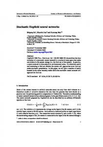
Figure 1: The state trajectories for open-loop SINNs (52) with initial condition 𝑥(0) = (−0.15, 0.2)𝑇 , 𝑦(0) = (0.3, 0.3)𝑇 .

𝑛

+ ∑ 𝑐𝑖𝑗 𝑓𝑗 (𝑥𝑗 (𝑡))

open−loop case

0.2

𝑌1𝑇 ,

(51)

𝑛

open−loop case

0.2

+ ∑ 𝑑𝑖𝑗 𝑓𝑗 (𝑥𝑗 (𝑡 − ℎj (𝑡))) 𝑗=1

0.15

+ 𝛽𝑖 (𝑡, 𝑥𝑖 (𝑡)) 𝜔̇ 𝑖 (𝑡) , which are equivalent to the following vector form:

0.1

d𝑦 (𝑡) = [−𝐴𝑦 (𝑡) − 𝐵𝑥 (𝑡) + 𝐶𝑓 (𝑥 (𝑡)) + 𝐷𝑓 (𝑥 (𝑡 − ℎ (𝑡))) + 𝑢 (𝑡)] d𝑡 + 𝛽 (𝑡, 𝑥 (𝑡)) d𝜔 (𝑡) , where 1 0 Ξ=( ), 0 3 2 0 𝐴=( ), 0 3

x2

d𝑥 (𝑡) = [−Ξ𝑥 (𝑡) + 𝑦 (𝑡) + ] (𝑡)] d𝑡,

0.05

(52) 0

−0.05 −0.16 −0.14 −0.12 −0.1 −0.08 −0.06 −0.04 −0.02 x1

𝑀1 = (

2 −5 𝐶=( ), −1 −3

𝑀2 = (

sin (𝑥1 + 𝑥2 ) 0 𝛽 (𝑡, 𝑥 (𝑡)) = ( ), 0 2 cos 2 (𝑥1 − 𝑥2 ) tanh (𝑥1 ) 𝑓 (𝑥 (𝑡)) = ( ), tanh (𝑥2 ) 0.25 sin (𝑡) + 0.75 ℎ (𝑡) = ( ), 0.25 sin (𝑡) + 0.75

0.02

Figure 2: The phrase trajectories for open-loop SINNs (52) with initial condition 𝑥(0) = (−0.15, 0.2)𝑇 , 𝑦(0) = (0.3, 0.3)𝑇 .

4 0 𝐵=( ), 0 6

1 −1 𝐷=( ), −1 −2

0

1 0 0 1

),

1 1 2 −2

). (53)

Setting the initial values 𝑥(0) = (−0.15, 0.2)𝑇 , 𝑦(0) = (0.3, 0.3)𝑇 , the state trajectories and phrase trajectories of the open-loop system are shown in Figures 1 and 2, respectively. Moreover, take 10 sets of numbers randomly as the initial values of 𝑥(0) and 𝑦(0) and satisfy 𝑥(0) ∈ (−1, 1), 𝑦(0) ∈ (−3, 3). Then the corresponding state trajectories and phrase trajectories of the open-loop system are shown in Figures 3 and 4, respectively. Obviously, the stochastic inertial neural networks with time-delay (51) are not finite-time stabilization.

8

Mathematical Problems in Engineering open−loop case

6

closed−loop case

2

4

1.5

2

1

x(t)

x(t)

0

0.5

−2 0 −4 −0.5

−6 −8

−1 0

1

2

3

4 5 t (seconds)

6

7

8

Figure 3: The state trajectories for open-loop SINNs (52) with 10 different initial conditions 𝑥(0) ∈ (−1, 1), 𝑦(0) ∈ (−3, 3).

1

2

3

4 5 t (seconds)

6

7

8

Figure 5: The state trajectories for closed-loop SINNs (52) with initial condition 𝑥(0) = (−1, 1)𝑇 , 𝑦(0) = (−3, 3)𝑇 . closed−loop case

2

open−loop case

0.6

0

1.5

0.4 0.2

1

x2

x2

0 −0.2

0.5

−0.4 0

−0.6 −0.8

−0.5 −1

−1 −0.8 −0.6 −0.4 −0.2

0

0.2 x1

0.4

0.6

0.8

1

Figure 4: The phrase trajectories for open-loop SINNs (52) with 10 different initial conditions 𝑥(0) ∈ (−1, 1), 𝑦(0) ∈ (−3, 3).

Hence, we need to design the delay-feedback controller as (44) for system (51), where the parameter 𝜇 is chosen as 0.6, and the initial values 𝑥(0) = (−1, 1)𝑇 , 𝑦(0) = (3, −3)𝑇,𝐾2 = ( 52 21 ), 𝐾4 = ( 32 24 ). The solution of (49) is derived by resorting to Matlab LMI Control Toolbox: 0.0793 0.0242 ), 𝑋1 = ( 0.0242 0.0712 0.5705 0.0492 ), 𝑋2 = ( 0.0492 0.6263 0.2766 0.0585 ), 𝑀3 = ( 0.0585 0.0399

−0.8

−0.6

−0.4

−0.2

0

0.2

0.4

x1

Figure 6: The phrase trajectories for closed-loop SINNs (52) with initial condition 𝑥(0) = (−1, 1)𝑇 , 𝑦(0) = (−3, 3)𝑇 .

0.3609 −9.9199 𝑌1 = ( ), 9.8791 0.2501 −0.5432 −5.9469 ), 𝑌2 = ( 5.4102 −1.0974 52.5297 152.1518 ), 𝐾1 = ( 137.7642 −43.3383 −0.1341 −9.4851 ). 𝐾3 = ( 9.6993 −2.5141 (54) 14.0697 −4.7821 ), 𝑃 = ( 1.7648 −0.1386 ), We can get 𝑃1 = ( −4.7821 2 15.6703 −0.1386 1.6076 𝑇0 ≤ 3.2211. The state trajectories and phrase trajectories of close-loop system are shown in Figures 5 and 6, respectively.


9

closed−loop case

1

closed−loop case

15

0.8

10

0.6 5

0.4

0 x(t)

x(t)

0.2 0

−5

−0.2 −0.4

−10

−0.6 −15

−0.8 −1

0

1

2

3

4 5 t (seconds)

6

7

−20

8

Figure 7: The state trajectories for closed-loop SINNs (52) with 100 different initial conditions 𝑥(0) ∈ (−1, 1), 𝑦(0) ∈ (−3, 3).

0

1

2

4 5 t (seconds)

6

7

8

Figure 9: The state trajectories for closed-loop SINNs (52) with 100 different initial conditions 𝑥(0) ∈ (−10, 10), 𝑦(0) ∈ (−30, 30).

closed−loop case

1

3

closed−loop case

60

0.8 50

0.6 0.4

40 30

0

x2

x2

0.2

−0.2

20

−0.4 10

−0.6

0

−0.8 −1 −1

−0.5

0 x1

0.5

1

Figure 8: The phrase trajectories for closed-loop SINNs (52) with 100 different initial conditions 𝑥(0) ∈ (−1, 1), 𝑦(0) ∈ (−3, 3).

In order to make the result of the simulation more convincing, we take 100 sets of numbers randomly as the initial values of 𝑥(0) and 𝑦(0) and satisfy 𝑥(0) ∈ (−1, 1), 𝑦(0) ∈ (−3, 3). Then the corresponding state trajectories are shown in Figure 7 and the corresponding phrase trajectories are shown in Figure 8. Obviously, the stochastic inertial neural networks with time-delay (51) are finite-time stabilization. Moreover, when 𝑥(0) ∈ (−10, 10), 𝑦(0) ∈ (−30, 30), we have state trajectories in Figure 9 and phrase trajectories in Figure 10, which also figure out that the stochastic inertial neural networks with time-delay (51) are finite-time stabilization.

−10 −100

−80

−60

−40

−20

20

40

Figure 10: The phrase trajectories for closed-loop SINNs (52) with 100 different initial conditions 𝑥(0) ∈ (−10, 10), 𝑦(0) ∈ (−30, 30).

stochastic inertial neural networks with or without timedelay. Provided that a set of LMIs are feasible, a suitable delayed or nondelayed nonlinear feedback controller can be designed such that finite-time stability in probability can be ensured for the system under study. An example has been given to demonstrate the correctness of the theoretical results and the effectiveness of the proposed methods.

Data Availability No data were used to support this study.

5. Conclusions In this work, by constructing a proper Lyapunov function, the finite-time stabilization problem has been addressed for

0

x1

Conflicts of Interest The authors declare no conflicts of interest.

10

Acknowledgments This work was supported by the Nation Natural Science Foundation of China under Grants 61473213 and 61671338.

References [1] S. G. Hu, Y. Liu, Z. Liu et al., “Associative memory realized by a reconfigurable memristive Hopfield neural network,” Nature Communications, vol. 6, article no. 8522, 2015. [2] J. Yang, L. Wang, Y. Wang, and T. Guo, “A novel memristive Hopfield neural network with application in associative memory,” Neurocomputing, vol. 227, pp. 142–148, 2017. [3] J. F. Durodola, N. Li, S. Ramachandra, and A. N. Thite, “A pattern recognition artificial neural network method for random fatigue loading life prediction,” International Journal of Fatigue, vol. 99, pp. 55–67, 2017. [4] X.-M. Zhang, Q.-L. Han, X. Ge, and D. Ding, “An overview of recent developments in Lyapunov-Krasovskii functionals and stability criteria for recurrent neural networks with timevarying delays,” Neurocomputing, 2018. [5] S. Xu and J. Lam, “A new approach to exponential stability analysis of neural networks with time-varying delays,” Neural Networks, vol. 19, no. 1, pp. 76–83, 2006. [6] X.-M. Zhang and Q.-L. Han, “Global asymptotic stability for a class of generalized neural networks with interval time-varying delay,” IEEE Trans. Neural Netw, vol. 22, pp. 1180–1192, 2011. [7] S.-P. Xiao, H.-H. Lian, H.-B. Zeng, G. Chen, and W.-H. Zheng, “Analysis on robust passivity of uncertain neural networks with time-varying delays via free-matrix-based integral inequality,” International Journal of Control, Automation, and Systems, vol. 15, no. 5, pp. 2385–2394, 2017. [8] X.-M. Zhang and Q.-L. Han, “Global asymptotic stability analysis for delayed neural networks using a matrix-based quadratic convex approach,” Neural Networks, vol. 54, pp. 57–69, 2014. [9] G. Chen, H. Wang, and Y. Yang, “Finite-time stabilization for stochastic delayed recurrent neural networks via nonlinear delay-feedback controller,” in Proceedings of the 2017 Chinese Automation Congress (CAC), pp. 1411–1416, Jinan, October 2017. [10] Y. Wei, J. H. Park, H. R. Karimi, Y.-C. Tian, and H. Jung, “Improved Stability and Stabilization Results for Stochastic Synchronization of Continuous-Time Semi-Markovian Jump Neural Networks With Time-Varying Delay,” IEEE Transactions on Neural Networks and Learning Systems, 2017. [11] S. Zhu, Y. Shen, and G. Chen, “Exponential passivity of neural networks with time-varying delay and uncertainty,” Physics Letters A, vol. 375, no. 2, pp. 136–142, 2010. [12] Z. Tu, J. Cao, and T. Hayat, “Matrix measure based dissipativity analysis for inertial delayed uncertain neural networks,” Neural Networks, vol. 75, pp. 47–55, 2016. [13] J. Wang, X.-M. Zhang, and Q.-L. Han, “Event-triggered generalized dissipativity filtering for neural networks with timevarying delays,” IEEE Transactions on Neural Networks and Learning Systems, vol. 27, no. 1, pp. 77–88, 2015. [14] D. Huang, M. Jiang, and J. Jian, “Finite-time synchronization of inertial memristive neural networks with time-varying delays via sampled-date control,” Neurocomputing, vol. 266, pp. 527– 539, 2017. [15] N. Cui, H. Jiang, C. Hu, and A. Abdurahman, “Finite-time synchronization of inertial neural networks,” Journal of the Association of Arab Universities for Basic and Applied Sciences, vol. 24, no. 1, pp. 300–309, 2018.

Mathematical Problems in Engineering [16] X. Zhang and Q. Han, “State estimation for static neural networks with time-varying delays based on an improved reciprocally convex inequality,” IEEE Transactions on Neural Networks and Learning Systems, pp. 1–6, 2017. [17] C. Lu, X. Zhang, M. Wu, Q. Han, and Y. He, “Energy-toPeak State Estimation for Static Neural Networks With Interval Time-Varying Delays,” IEEE Transactions on Cybernetics, vol. 48, no. 10, pp. 2823–2835, 2018. [18] S. Zhang, Y. Yu, and Q. Wang, “Stability analysis of fractionalorder Hopfield neural networks with discontinuous activation functions,” Neurocomputing, vol. 171, pp. 1075–1084, 2016. [19] R. J. Williams and D. Zipser, “A learning algorithm for continually running fully recurrent neural networks,” Neural Computation, vol. 1, no. 2, pp. 270–280, 1989. [20] Z. Tu, J. Cao, and T. Hayat, “Global exponential stability in Lagrange sense for inertial neural networks with time-varying delays,” Neurocomputing, vol. 171, pp. 524–531, 2016. [21] K. L. Babcock and R. M. Westervelt, “Stability and dynamics of simple electronic neural networks with added inertia,” Physica D: Nonlinear Phenomena, vol. 23, no. 1-3, pp. 464–469, 1986. [22] R. Sakthivel, R. Samidurai, and S. . Anthoni, “Exponential stability for stochastic neural networks of neural type with impulsive effects,” Modern Physics Letters B. Condensed Matter Physics, Statistical Physics, Applied Physics, vol. 24, no. 11, pp. 1099–1110, 2010. [23] F. Wang, Y. Chen, and M. Liu, “pth moment exponential stability of stochastic memristor-based bidirectional associative memory (BAM) neural networks with time delays,” Neural Networks, vol. 98, pp. 192–202, 2018. [24] Q. Zhu, C. Huang, and X. Yang, “Exponential stability for stochastic jumping BAM neural networks with time-varying and distributed delays,” Nonlinear Analysis: Hybrid Systems, vol. 5, no. 1, pp. 52–77, 2011. [25] Z. Meng and Z. Xiang, “Stability analysis of stochastic memristor-based recurrent neural networks with mixed timevarying delays,” Neural Computing and Applications, pp. 1–13, 2016. [26] J. L. Yin, S. Khoo, Z. H. Man, and X. H. Yu, “Finite-time stability and instability of stochastic nonlinear systems,” Automatica, vol. 47, no. 12, pp. 2671–2677, 2011. [27] X. Song and X. Yan, “Linear quadratic Gaussian control for linear time-delay systems,” IET Control Theory & Applications, vol. 8, no. 6, pp. 375–383, 2014. [28] X. Yan, X. Song, and X. Wang, “Global output-feedback stabilization for nonlinear time-delay systems with unknown control coefficients,” International Journal of Control, Automation, and Systems, vol. 16, no. 4, pp. 1550–1557, 2018. [29] X. Liu, N. Jiang, J. Cao, S. Wang, and Z. Wang, “Finitetime stochastic stabilization for BAM neural networks with uncertainties,” Journal of The Franklin Institute, vol. 350, no. 8, pp. 2109–2123, 2013. [30] F. Xiao, L. Wang, J. Chen, and Y. Gao, “Finite-time formation control for multi-agent systems,” Automatica, vol. 45, no. 11, pp. 2605–2611, 2009. [31] J. Cortés, “Finite-time convergent gradient flows with applications to network consensus,” Automatica, vol. 42, no. 11, pp. 1993–2000, 2006. [32] G. Chen, F. L. Lewis, and L. Xie, “Finite-time distributed consensus via binary control protocols,” Automatica, vol. 47, no. 9, pp. 1962–1968, 2011.

Mathematical Problems in Engineering [33] J. Lu, D. W. C. Ho, and Z. Wang, “Pinning stabilization of linearly coupled stochastic neural networks via minimum number of controllers,” IEEE Transactions on Neural Networks and Learning Systems, vol. 20, no. 10, pp. 1617–1629, 2009. [34] X. Li, “New results on global exponential stabilization of impulsive functional differential equations with infinite delays or finite delays,” Nonlinear Analysis: Real World Applications, vol. 11, no. 5, pp. 4194–4201, 2010. [35] J. Yin and S. Khoo, “Comments on finite-time stability theorem of stochastic nonlinear systems,” Automatica, vol. 47, no. 7, pp. 1542-1543, 2011. [36] B. Zhang, Q. Han, X. Zhang, and Yu. X, “Sliding mode control with mixed current and delayed states for offshore steel jacket platform,” IEEE Trans. Control Syst. Technol, vol. 22, pp. 1769– 1783, 2014. [37] B.-L. Zhang, Q.-L. Han, and X.-M. Zhang, “Recent advances in vibration control of offshore platforms,” Nonlinear Dynamics, vol. 89, no. 2, pp. 755–771, 2017. [38] S. Xiao, L. Xu, H. Zeng, and K. L. Teo, “Improved Stability Criteria for Discrete-time Delay Systems via Novel Summation Inequalities,” International Journal of Control, Automation, and Systems, vol. 16, no. 4, pp. 1592–1602, 2018.

11

Advances in

Operations Research Hindawi www.hindawi.com

Volume 2018

Advances in

Decision Sciences Hindawi www.hindawi.com

Volume 2018

Journal of

Applied Mathematics Hindawi www.hindawi.com

Volume 2018

The Scientific World Journal Hindawi Publishing Corporation http://www.hindawi.com www.hindawi.com

Volume 2018 2013

Journal of

Probability and Statistics Hindawi www.hindawi.com

Volume 2018

International Journal of Mathematics and Mathematical Sciences

Journal of

Optimization Hindawi www.hindawi.com

Hindawi www.hindawi.com

Volume 2018

Volume 2018

Submit your manuscripts at www.hindawi.com International Journal of

Engineering Mathematics Hindawi www.hindawi.com

International Journal of

Analysis

Journal of

Complex Analysis Hindawi www.hindawi.com

Volume 2018


Stochastic Analysis Hindawi www.hindawi.com


Volume 2018

Volume 2018

Advances in

Numerical Analysis Hindawi www.hindawi.com

Volume 2018

Journal of


Volume 2018

Journal of

Mathematics Hindawi www.hindawi.com


Function Spaces Volume 2018


Volume 2018


Differential Equations Hindawi www.hindawi.com

Volume 2018

Abstract and Applied Analysis Hindawi www.hindawi.com

Volume 2018

Discrete Dynamics in Nature and Society Hindawi www.hindawi.com

Volume 2018

Advances in

Mathematical Physics Volume 2018


Volume 2018