My Background. ▻ Mid 1980's: PhD student studying discrete-event simulation ...
SPNs as a modelling framework for discrete-event systems. ▻ Sample path ...
STOCHASTIC PETRI NETS FOR DISCRETE-EVENT SIMULATION Peter J. Haas IBM Almaden Research Center San Jose, CA
Petri Nets 2007
Part I Introduction
2
Peter J. Haas
Petri Nets 2007
My Background I
Mid 1980’s: PhD student studying discrete-event simulation I
I
I
I
I I I I
3
“Regenerative simulation of stochastic Petri nets”
Kept working (in between Info. Mgmt. research) . . . I
I
“Performance analysis using stochastic Petri nets”
Wrote PNPM85 simulation paper with Gerry Shedler I
I
Under Donald Iglehart (Stanford) & Gerald Shedler (IBM)
Saw Michael Molloy 1982 paper in IEEE Trans. Comput.:
Modelling power for simulation [HS88] Prototypes: SPSIM, “Labelled” SPN simulator [JS89, HS90] Delays [HS93a,b] Standardized time series [Haa97,99a,99b] Transience and recurrence [GH06, GH07]
Gave this seminar at 2004 Winter Simulation Conference
Peter J. Haas
Petri Nets 2007
Complex Systems
4
Peter J. Haas
Petri Nets 2007
Simulation and SPNs I
Assessment of system performance is difficult I I
Even modelling the system is hard! Model is usually analytically and numerically intractable I
I
I
I
But can’t simulate blindly
SPNs can help I I I
5
Huge state space and/or non-Markovian
Simulation is often the only available numerical method
An attractive graphically-oriented modelling framework Well suited to sample-path generation on a computer Solid mathematical foundation
Peter J. Haas
Petri Nets 2007
This Tutorial
Simulation theory for SPNs
6
I
SPNs as a modelling framework for discrete-event systems
I
Sample path generation for SPNs
I
Steady-state output analysis: theory and methods
Peter J. Haas
Petri Nets 2007
Sources for This Tutorial
I
I
7
“Law of large numbers and functional central limit theorem for generalized semi-Markov processes.” P. W. Glynn and P. J. Haas. Comm. Statist. Stochastic Models, 22(2), 2006, 201–232. On Transience and Recurrence in Irreducible Finite-State Stochastic Systems. P. W. Glynn and P. J. Haas. IBM Technical Report, 2007.
Peter J. Haas
Petri Nets 2007
Outline I
Simulation basics I I
I
Modelling with SPNs I I
I
I
The marking process Efficiency issues, parallelism
Steady-state estimation for SPNs I I
8
Building blocks Modeling power for simulation
Sample-path generation I
I
Discrete-event systems The simulation process
Conditions for long-run stability (recurrence, limit theorems) Output-analysis methods and their validity
Peter J. Haas
Petri Nets 2007
Goals
9
I
Illustrate the rich behavior of non-Markvian SPNs
I
Introduce you to some basic simulation methodology
I
Explore foundational issues in modelling and analysis
I
Connect modeling practice and simulation theory
I
Stimulate your interest in SPNs as a simulation framework
Peter J. Haas
Petri Nets 2007
Part II Simulation Basics
10
Peter J. Haas
Petri Nets 2007
What We Simulate: Discrete-Event Stochastic Systems
I
System changes state when events occur I
I
Underlying stochastic process { X (t) : t ≥ 0 } I I I
I
X (t) = state of system at time t (a random variable) Piecewise-constant sample paths Typically not a continuous-time Markov chain
Modelling challenge: defining appropriate system state I I I
11
Stochastic changes at random times
Compact for efficiency reasons Enough info to compute performance measures Enough info to determine evolution
Peter J. Haas
Petri Nets 2007
Why We Simulate: Performance Evaluation I
Steady-state performance measures I
Time-average limits: α = lim
t→∞
I
1 t
Z
t
� f X (u) du
0
Steady-state means: α = E [f (X )], where X (t) ⇒ X I
I
Want point estimate α ˆ (t) I I
I
Unbiased: Eµ [ˆ α(t)] = α Strongly consistent: Pµ { limt→∞ α ˆ (t) = α } = 1
Want asymptotic 100p% confidence interval I
I (t) = [α ˆ (t) − H(t), α ˆ (t) + H(t)]
I
Pµ { I (t) 3 α } ≈ p for large t CI width indicates precision of point estimate
I
12
I.e., Pµ { X (t) = s } → P { X = s } as t → ∞
Peter J. Haas
Petri Nets 2007
Challenges in Performance Evaluation I
Is steady-state quantity α well-defined? I
I
Is steady-state quantity independent of startup condition µ? I
I
Ex: reducible Markov chain
Statistical challenges I I
I
Ex: steady-state number in M/M/1 queue with ρ > 1
Autocorrelation problem Initialization bias problem
How to handle Delays? n−1 1X f (Dj ) n→∞ n
lim
j=0
13
Peter J. Haas
Petri Nets 2007
The Simulation Process
14
Peter J. Haas
Petri Nets 2007
How Modelling Frameworks Can Help
I
But challenges, also: I
15
Immediate transitions and markings
Peter J. Haas
Petri Nets 2007
Part III Modelling with SPNs
16
Peter J. Haas
Petri Nets 2007
The SPN Graph d1
d2
s = (2, 1, 1) d3
17
I
D = finite set of places
I
E = finite set of transitions (timed and immediate)
I
marking = assignment of token counts to places
Peter J. Haas
Petri Nets 2007
Transition Firing
p(s 0 ; s, e ∗ )
18
I
The marking changes when an enabled transition fires
I
Removes 1 token per place from random subset of input places
I
Deposits 1 token per place in random subset of output places
Peter J. Haas
Petri Nets 2007
Clocks (Event Scheduling)
I I
One clock per transition: records remaining time until firing Enabled transitions compete to trigger marking change I I I
I
At a marking change: three kinds of transitions I I I
19
The clock that runs down to 0 first is the “winner” Can have simultaneous transition firing: p(s 0 ; s, E ∗ ) Numerical priorities: specify simultaneous-firing behavior New transitions: Use clock-setting distribution function Old transitions: Clocks continue to run down Newly-disabled transitions: Clock readings are discarded
Peter J. Haas
Petri Nets 2007
Clocks, Continued
I
Clock-setting distribution depends on: I
I
Clocks run down at marking-dependent speeds r (s, e) I I
20
Old marking, new marking, trigger set Processor sharing Zero speeds: preempt-resume behavior
Peter J. Haas
Petri Nets 2007
Timed and Immediate Markings
21
I
Immediate marking: ≥ 1 immediate transition is enabled
I
An immediate marking vanishes as soon as it is attained
I
Otherwise, marking is timed
Peter J. Haas
Petri Nets 2007
Example: Cyclic Queues with Feedback
22
Peter J. Haas
Petri Nets 2007
Bottom-Up and Top-Down Modeling
23
Peter J. Haas
Petri Nets 2007
Other Modeling Features
24
Concurrency:
Synchronization:
Precedence:
Priority:
Peter J. Haas
Petri Nets 2007
Why This SPN Model?
I I
Conciseness: small set of building blocks Generality: subsumes GSPNs, etc. I
I
25
Theory carries over
Modelling power: captures many discrete-event systems
Peter J. Haas
Petri Nets 2007
Modeling Power of SPNs I
Compare to Generalized semi-Markov processes (GSMPs) I I I I
I
Strong mimicry I I I I
I
Define X (t) = state of system at time t Define (Sn , Cn ) = (state, clocks) after nth state transition { X (t) : t ≥ 0 } processes have same dist’n (under mapping) { (Sn , Cn ) : n ≥ 0 } have same dist’n (under mapping)
Theorem: SPNs and GSMPs have same modeling power I I I
26
Arbitrary state definition (s) Set E (s) of active events is a building block No restrictions on p(s 0 ; s, E ∗ ) No “immediate events”
Establishes SPNs as framework for discrete-event simulation Allows application of GSMP theory to SPNs Methodology allows other comparisons (e.g., inhibitor arcs)
Peter J. Haas
Petri Nets 2007
Part IV Sample-Path Generation
27
Peter J. Haas
Petri Nets 2007
The Marking Process
I
Marking process: { X (t) : t ≥ 0 } I I
I
Defined in terms of Markov chain { (Sn , Cn ) : n ≥ 0 } I I I I
28
X (t) = the marking at time t A very complicated process System observed after the nth marking change Sn = (Sn,1 , . . . , Sn,L ) = the marking Cn = (Cn,1 , . . . , Cn,M ) = the clock-reading vector Chain defined via SPN building blocks
Peter J. Haas
Petri Nets 2007
Definition of the Marking Process
29
Peter J. Haas
Petri Nets 2007
Generation of the GSSMC { (Sn , Cn ) : n ≥ 0 } 1. [Initialization] Set n = 0. Select marking S0 and clock readings C0,i for ei ∈ E (S0 ); set C0,i = −1 for ei 6∈ E (S0 ). 2. Determine holding time t ∗ (Sn , Cn ) and firing set En∗ . 3. Generate new marking Sn+1 according to p( · ; Sn , En∗ ). 4. Set clock-reading Cn+1,i for each new transition ei according to F ( · ; Sn+1 , ei , Sn , En∗ ). 5. Set clock-reading Cn+1,i for each old transition ei as Cn+1,i = Cn,i − t ∗ (Sn , Cn )r (Sn , ei ). 6. Set clock-reading Cn+1,i equal to −1 for each newly disabled transition ei . 7. Set n ← n + 1 and go to Step 2. Can compute GSMP { X (t) : t ≥ 0 } from GSSMC
30
Peter J. Haas
Petri Nets 2007
Implementation Considerations for Large-Scale SPNs I
Use event lists (e.g., heaps) to determine E ∗ I I
I I
Updating the state is often simpler in an SPN Efficient techniques for event scheduling [Chiola91] I
I
Encode transitions potentially affected by firing of ei
Parallel simulation of subnets I I I
31
O(1) computation of E ∗ � O log m update time, where m = # of enabled transitions
E.g., Adaptive Time Warp [Ferscha & Richter PNPM97] Guardedly optimistic Slows down local firings based on history of rollbacks Peter J. Haas
Petri Nets 2007
Part V Stability Theory for SPNs
32
Peter J. Haas
Petri Nets 2007
Stability and Simulation I
Focus on time-average limits: 1 r (f ) = lim t→∞ t
I I
I I
I I
33
� f X (u) du
0
1 X˜ f (Sn , Cn ) ˜r (f˜) = lim n→∞ n i=0
Functions (e.g. ratios) of such limits Cumulative rewards (impulse/continuous/mixed), gradients Steady-state means
Key questions: I
I
n−1
t
Ex: long-run cost, availability, utilization Extensions: I
I
Z
When do such limits exist? When do various estimation methods apply? Can get weird behavior: limn E [ζn − ζn−1 ] = ∞ but explodes!
Approach: analyze the chain { (Sn , Cn ) : n ≥ 0 } Peter J. Haas
Petri Nets 2007
Harris Recurrence: A Basic Form of Stability I
Definition for general chain { Zn : n ≥ 0 } with state space Γ Pz { Zn ∈ A i.o. } = 1, z ∈ Γ
I I I
I
I I
Chain admits invariant probability measure π Pπ { Z1 ∈ A } = π(A) Implies stationarity when initial dist’n is π
When is { (Sn , Cn ) : n ≥ 0 } (positive) Harris recurrent? I
34
φ is a recurrence measure (often “Lebesgue-like”) Every “dense enough” set is hit infinitely often w.p. 1 No “wandering off to ∞”
Positive Harris recurrence: I
I
whenever φ(A) > 0
Fundamental question for steady-state estimation
Peter J. Haas
Petri Nets 2007
Some Stability Conditions I
Density component g of a cdf F : F (t) ≥ s0
p(s 0 ; s, e)
Rt 0
g (u) du
I
s→
I
s; either s → s 0 or s → s (1) → · · · → s (n) → s 0 Assumption PD(q):
I
iff
I I I I
Marking set G is finite SPN is irreducible: s ; s 0 for all s, s 0 ∈ G All speeds are positive There exists x¯ ∈ (0, ∞) s.t. all clock-setting dist’n functions I I
I
> 0 for some e
s 0:
Have finite qth moment Have density component positive on [0, x¯]
Assumption PDE: replace finite qth moment requirement by Z ∞ e ux dF (x) < ∞ for u ∈ [0, aF ] 0
35
Peter J. Haas
Petri Nets 2007
Harris Recurrence in SPNs I
I
Embedded chain: { (Sn , Cn ) : n ≥ 0 } observed only at transitions to timed markings ¯ φ({s} × A) = Lebesgue measure of A ∩ [0, x¯]M
I
Theorem: If Assumption PD(1) holds, then the embedded chain is positive Harris recurrent with recurrence measure φ¯
I
Implies Pµ { Sn = s i.o. } = 1 for all s ∈ S Proof:
I
I I I I
I
Alternate approach to recurrence: geometric-trials arguments I I
36
First assume no immediate transitions ¯ Show that embedded chain is “φ-irreducible” Establish Lyapunov drift condition and apply MC machinery Extend to case of immediate transitions using strong mimicry Can drop positive-density assumption Use detailed analysis of specific SPN structure
Peter J. Haas
Petri Nets 2007
A Surprising Recurrence Result [Glynn and Haas 2007]
I I
Sn = marking just after nth marking change Conjecture: P { Sn = s i.o. } = 1 for each s if I I I
I
CONJECTURE IS FALSE! I
37
Marking set S is finite SPN is irreducible ∃ x¯ > 0 s.t. each F ( · ; e) has positive density on (0, x¯) In the presence of heavy-tailed clock-setting dist’ns
Peter J. Haas
Petri Nets 2007
The Counterexample I
S = { (2, 1, 1), (1, 2, 1), (1, 1, 2) }
I
p(s 0 ; s, e ∗ ) = 0 or 1 (see schematic diagram) Clock-setting distributions:
I
I I I
I
with β > 1/2 and α + β < 1 SPN hits marking s = (1, 2, 1) only if: I I
I
38
F (t; e1 ) = 1 − (1 + t)−α F (t; e2 ) = 1 − (1 + t)−β F ( · ; e3 ) is Uniform[0, a]
e1 occurs and then e2 occurs No intervening occurrence of e3
Theorem: P { Sn = (1, 2, 1) i.o. } = 0
Peter J. Haas
Petri Nets 2007
Another Type of Stability: Limit Theorems I
Theorem (SLLN): If Assumption PD(1) holds, then for any f Z � 1 t lim f X (u) du = r (f ) a.s. t→∞ t 0
I
Theorem (FCLT): If Assumption PD(2) holds, then for any f Uν (f ) ⇒ σ(f )W
I I I I
I I
� � R νt � Uν (f )(t) = ν −1/2 0 f X (u) − r (f ) du ⇒ denotes weak convergence on C [0, ∞) W = standard Brownian motion on [0, ∞) “Functional” form of CLT (ordinary CLT is a special case)
Note: r (f ) and σ(f ) are independent of initial conditions Follows from general result in [Glynn and Haas 2006] I
39
as ν → ∞
Uses results for Harris recurrent MCs Peter J. Haas
Petri Nets 2007
FCLT Example: Donsker’s Theorem
Sn =
40
Pn
i=0 Xi
Peter J. Haas
Petri Nets 2007
Part VI Steady-State Simulation
41
Peter J. Haas
Petri Nets 2007
Regenerative Simulation: Regenerative Processes
I I
A regenerative process can be decomposed into i.i.d. cycles System “probabilistically restarts” at each Ti I
I I
Analogous definition for discrete-time process { Xn : n ≥ 0 } Extension: one-dependent cycles I
42
Ex: successive arrival times to an empty GI/G/1 queue
Harris recurrent chains are od-regenerative (basis for previous SLLN and FCLT)
Peter J. Haas
Petri Nets 2007
Regenerative Simulation: The Ratio Formula I
Let
Ti
Z
� f X (u) du
Yi =
and τi = Ti − Ti−1
Ti−1 I
(Y1 , τ1 ), (Y2 , τ2 ), . . . are i.i.d. pairs
I
It follows that Pn Z Tn � Yi Y¯n 1 E [Y1 ] def = → =r f X (u) du = Pi=1 n Tn 0 τ¯n E [τ1 ] i=1 τi almost surely as n → ∞ (need E [τ1 ] < ∞)
I
Can show that 1 t
I
43
Z
t
� f X (u) du → r a.s. as t → ∞
0
If τ1 is “aperiodic”, then X (t) ⇒ X and E [f (X )] = r Peter J. Haas
Petri Nets 2007
Regenerative Simulation: The Regenerative Method I
Point estimate (biased): ˆrn = Y¯n /¯ τn :
I
Confidence interval
I
I I I
I
ˆrn → r a.s. as n → ∞ (strong consistency) Set Zi = Yi − r τi Z1 , Z2 , . . . i.i.d. with E [Zi ] = 0 and Var[Z1 ] = σ 2 Apply Central Limit Theorem (CLT) for i.i.d. random variables: � � √ √ n ˆrn − r n ˆrn − r ⇒ N(0, 1) and ⇒ N(0, 1) σ/E [τ1 ] sn /¯ τn as n → ∞, where sn estimates σ (we assume σ 2 < ∞) 100p% asymptotic confidence interval: � � zp sn zp sn ˆrn − √ , ˆrn + √ , τ¯n n τ¯n n where P { −zp ≤ N(0, 1) ≤ zp } = p, i.e., (1 + p)/2 quantile
I
44
Many extensions: bias reduction, fixed-time or fixed-precision, generalized Y and τ , estimate α = g (E [Y ] , E [τ ]), . . . Peter J. Haas
Petri Nets 2007
Regenerative Simulation of SPNs I
A marking ¯s is a single state if E (¯s ) = { e¯ }
I
Define θ(k) = kth marking change at which e¯ fires in ¯s
I
Set Tk = ζθ(k) and τk = Tk − Tk−1
I
Theorem: Suppose Assumption PD(2) holds and SPN has a single state ¯s I
I I
I I
Can therefore apply standard regenerative method Variant theorems are available I I I
45
Random times { Tk : k ≥ 0 } form sequence of regeneration points for marking process Finite expected cycle length: Eµ [τ1 ] < ∞ Finite variance constant for any f : � � �R T σ 2 (f ) = Varµ T01 f X (u) du − r τ1 < ∞
Variants of single state (e.g., memoryless property) Other recurrence conditions (geometric trials) Discrete-time results Peter J. Haas
Petri Nets 2007
The Method of Batch Means I
Simulate system to (large) time t = mv (where 10 ≤ m ≤ 20)
I
Divide into m batches of length v and compute batch means: 1 Y¯i = v
I
Z
iv
� f X (u) du
(i−1)v
Treat Y¯1 , Y¯2 , . . . , Y¯m as i.i.d., N(µ, σ 2 ): I I
Pm Point estimate: ˆrt = (1/m) i=1 Y¯i 100p% confidence interval: � � tp,m−1 sm tp,m−1 sm ˆrt − √ , ˆrt + √ , m m where tp,m−1 = (1 + p)/2 quantile of Student’s T dist’n
46
Peter J. Haas
Petri Nets 2007
Batch Means, Continued
I I
Why might batch means work? Formally, want to show I I I
I
47
Consistency of ˆrt and validity of CI as t → ∞ For m fixed (standard batch means) What if m = m(t)? Overlapping batches?
Special case of standardized-time-series methods
Peter J. Haas
Petri Nets 2007
Standardized Time Series I
Consider a mapping ξ : C [0, 1] 7→ < such that I I
ξ(ax) = aξ(x) and ξ(x − be) = ξ(x), where e(t) = t P { ξ(W ) > 0 } = 1 and P { W ∈ D(ξ) } = 0
R νt
I
Set Y¯ν (t) = (1/ν)
I
Theorem: If Assumption PD(2) holds, then r exists and √ σW (1) W (1) ˆrν − r ν(ˆrν − r ) = √ ¯ ⇒ = , ¯ σξ(W ) ξ(W ) ξ(Yν ) ξ( ν(Yν − re))
0
� f X (u) du and ˆrν = Y¯ν (1)
so that an asymptotic 100p% confidence interval for r is � � ˆrν − ξ(Y¯ν )zp , ˆrν + ξ(Y¯ν )zp ,
I
where P{ −zp ≤ W (1)/ξ(W ) ≤ zp } = p Different choices of ξ yield different estimation methods I I
48
batch means (fixed # of batches) STS area method, STS maximum method Peter J. Haas
Petri Nets 2007
Consistent-Estimation Methods (Discrete Time) I
Set ˆrn = (1/n)
Pn−1 ˜ j=0 f (Sj , Cj ) and suppose that √
lim ˆrn = ˜r a.s. and
n→∞ I
If we can find a consistent estimator Vn ⇒ σ ˜ 2 , then � √ n ˆrn − ˜r ⇒ N(0, 1) 1/2 Vn
I
Then an asymptotic 100p% confidence interval for ˜r is " # 1/2 1/2 zp Vn zp Vn , ˆrn + √ , ˆrn − √ n n
I 49
� n ˆrn − ˜r ⇒ N(0, 1) σ ˜
where zp = (1 + p)/2 quantile of N(0, 1) Narrower asymptotic confidence intervals than STS methods Peter J. Haas
Petri Nets 2007
Consistent-Estimation Methods for SPNs I
Look at polynomially dominated functions: f˜(s, c) = O(1 + max1≤i≤M ciq ) for some q ≥ 0
I
Require aperiodicity: no partition of marking set G s.t. G1 → G2 → · · · → Gd → G1 → G2 → · · · Focus on “localized quadratic-form variance estimators”
I
I
Quadratic-form: Vn =
n X n X
(n) f˜(Si , Ci )f˜(Sj , Cj )qi,j
i=0 j=0 I
Localized: (n) |qi,j |
( a1 /n ≤ a2 (n)/n
if |i − j| ≤ m(n); if |i − j| > m(n)
where a2 (n) → 0 and m(n)/n → 0 50
Peter J. Haas
Petri Nets 2007
Exploiting Results for Stationary Output
I
Theorem: For an aperiodic SPN, suppose that I I I I
I
Then Vn ⇒ σ ˜ 2 for any initial distribution Proof: I I
I
51
Assumption PDE holds (∃ invariant distribution π) { f˜(Sn , Cn ) : n ≥ 0 } obeys a CLT with variance constant σ ˜2 2 Vn is a localized quadratic-form estimator of σ ˜ Vn ⇒ σ ˜ 2 when initial distribution = π
{ (Sn , Cn ) : n ≥ 0 } couples with stationary version Localization: difference between Vn versions becomes negligible
Consequence: can exploit existing consistency results for stationary output
Peter J. Haas
Petri Nets 2007
Coupling Harris-Ergodic Markov Chains
52
Peter J. Haas
Petri Nets 2007
Application to Specific Variance Estimators I
Variable batch means estimator of σ ˜2: I I
I
Spectral estimator of σ ˜2: I I I I I
53
b(n) batches of m(n) observations each VBM estimator is consistent if Assumption PDE holds, f˜ is polynomially dominated, b(n) → ∞, and m(n) → ∞. Pm−1 (S) ˆh Form of estimator: Vn = h=−(m−1) λ(h/m)R ˆ h = sample lag-h autocorrelation of { f˜(Sn , Cn ) : n ≥ 0 } R λ( · ) = “regular” window function (Bartlett, Hanning, Parzen) m = m(n) = spectral window length Spectral estimator is consistent if Assumption PDE holds, f˜ is polynomially dominated, m(n) → ∞, and m(n)/n1/2 → 0
I
Overlapping batch means: asymp. equivalent to spectral
I
Can extend results to continuous time (and drop aperiodicity)
Peter J. Haas
Petri Nets 2007
Estimation of Delays in SPNs Want to estimate limn→∞ (1/n)
I
Delays D0 , D1 , . . . “determined by marking changes of the net” Specified as Dj = Bj − Aj
I
I I I
I
I I I
I
j=0
f (Dj )
� Starts: Aj = �ζα(j) : j ≥ 0 nondecreasing Terminations: Bj = ζβ(j) : j ≥ 0 Determined by { (Sn , Cn ) : n ≥ 0 }
Measuring lengths of delay intervals is nontrivial I
54
Pn−1
I
Must link starts and terminations Multiple ongoing delays Overtaking: delays need not terminate in start order Pn−1 Can avoid for limiting average delay limn→∞ (1/n) j=0 Dj
Measurement methods: tagging and start vectors
Peter J. Haas
Petri Nets 2007
Tagging
55
Peter J. Haas
Petri Nets 2007
Start Vectors
I
Assume # of ongoing delays = ψ(s) when marking is s
I
Vn records starts for all ongoing delays at ζn
I
Positions of starts = position of entities in system (usually)
I
Use -1 as placeholder At each marking change:
I
I I I I
56
Insert current time according to iα (s 0 ; s, E ∗ ) Delete components according to iβ (s 0 ; s, E ∗ ) Permute components according to iπ (s 0 ; s, E ∗ ) Subtract deleted components from current time to compute delays (ignore -1’s)
Peter J. Haas
Petri Nets 2007
Start Vector Example
57
Peter J. Haas
Petri Nets 2007
Regenerative Methods: The Easy Case
58
I
Assume SPN has single state and “well behaved” cycles
I
Use standard regenerative method
Peter J. Haas
Petri Nets 2007
Regenerative Methods: The Hard Case
59
I
Assume SPN has single state and “well behaved” cycles
I
Decompose delays into one-dependent cycles
I
Use extended regenerative method or multiple-runs method
Peter J. Haas
Petri Nets 2007
Limiting Average Delay I
Under appropriate regularity conditions n−1
Eµ [Z1 ] 1X Dj = a.s. n→∞ n Eµ [δ1 ] lim
j=0
I I I I
60
δ1 = # R of starts in� regenerative cycle Z1 = cycle ψ X (t) dt ψ(s) = # of ongoing delays when marking is s (Z1 , δ1 ), (Z2 , δ2 ), . . . are i.i.d.
I
Can use standard regenerative method
I
No need to measure individual delays
I
One proof of this result uses Little’s Law
Peter J. Haas
Petri Nets 2007
STS Methods for Delays I
Focus on “regular” start-vector mechanism
I
Use polynomially-dominated functions f :