Stochastic Phase Dynamics in Neuron Models and ... - Semantic Scholar

Stochastic Phase Dynamics in Neuron Models and Spike Time Reliability by Na Yu B.Sc., Hebei University, 1999 M.Sc., University of Science and Technology Beijing, 2002 A THESIS SUBMITTED IN PARTIAL FULFILLMENT OF THE REQUIREMENTS FOR THE DEGREE OF DOCTOR OF PHILOSOPHY in The Faculty of Graduate Studies (Mathematics)

THE UNIVERSITY OF BRITISH COLUMBIA (Vancouver) April, 2009 c Na Yu 2009

Abstract The present thesis is concerned with the stochastic phase dynamics of neuron models and spike time reliability. It is well known that noise exists in all natural systems, and some beneficial effects of noise, such as coherence resonance and noise-induced synchrony, have been observed. However, it is usually difficult to separate the effect of the nonlinear system itself from the effect of noise on the system’s phase dynamics. In this thesis, we present a stochastic theory to investigate the stochastic phase dynamics of a nonlinear system. The method we use here, called “the stochastic multi-scale method”, allows a stochastic phase description of a system, in which the contributions from the deterministic system itself and from the noise are clearly seen. Firstly, we use this method to study the noise-induced coherence resonance of a single quiescent “neuron” (i.e. an oscillator) near a Hopf bifurcation. By calculating the expected values of the neuron’s stochastic amplitude and phase, we derive analytically the dependence of the frequency of coherent oscillations on the noise level for different types of models. These analytical results are in good agreement with numerical results we obtained. The analysis provides an explanation for the occurrence of a peak in coherence measured at an intermediate noise level, which is a defining feature of the coherence resonance. Secondly, this work is extended to study the interaction and competition of the coupling and noise on the synchrony in two weakly coupled neurons. Through numerical simulations, we demonstrate that noise-induced mixed-mode oscillations occur due to the existence of multistability states for the deterministic oscillators with weak coupling. We also use the standard multi-scale method to approximate the multistability states of a normal form of such a weakly coupled system. Finally we focus on the spike time reliability that refers to the phenomenon: the repetitive application of a stochastic stimulus to a neuron generates spikes with remarkably reliable timing whereas repetitive injection of a constant current fails to do so. In contrast to many numerical and experimental studies in which parameter ranges corresponding to repetitive spiking, we show that the intrinsic frequency of extrinsic noise has no direct relationship with spike time reliability for parameters corresponding to quiescent ii

states in the underlying system. We also present an “energy” concept to explain the mechanism of spike time reliability. “Energy” is defined as the integration of the waveform of the input preceding a spike. The comparison of “energy” of reliable and unreliable spikes suggests that the fluctuation stimuli with higher ”energy” generate reliable spikes. The investigation of individual spike-evoking epochs demonstrates that they have a more favorable time profile capable of triggering reliably timed spike with relatively lower energy levels.

iii

Table of Contents . . . . . . . . . . . . . . . . . . . . . . . . . . . . . . . . .

ii

Table of Contents . . . . . . . . . . . . . . . . . . . . . . . . . . . .

iv

Abstract

List of Tables

. . . . . . . . . . . . . . . . . . . . . . . . . . . . . . vii

List of Figures . . . . . . . . . . . . . . . . . . . . . . . . . . . . . . viii List of Abbreviations

. . . . . . . . . . . . . . . . . . . . . . . . . xv

Acknowledgements . . . . . . . . . . . . . . . . . . . . . . . . . . . xvi Statement of Co-Authorship . . . . . . . . . . . . . . . . . . . . . xvii 1 Introduction . . . . . . . . . . . 1.1 Overview . . . . . . . . . . . 1.1.1 Coherence Resonance 1.1.2 Stochastic Synchrony 1.1.3 Spike Time Reliability 1.2 Objectives . . . . . . . . . . 1.3 Methods . . . . . . . . . . . 1.3.1 Analytical Method . 1.3.2 Numerical Methods .

. . . . . . . . .

1 2 2 4 6 7 9 9 12

Bibliography . . . . . . . . . . . . . . . . . . . . . . . . . . . . . . .

13

2

. . . . . . . .

. . . . . . . . .

. . . . . . . . .

. . . . . . . . .

. . . . . . . . .

. . . . . . . . .

. . . . . . . . .

. . . . . . . . .

. . . . . . . . .

. . . . . . . . .

. . . . . . . . .

. . . . . . . . .

. . . . . . . . .

Stochastic phase dynamics: multi-scale behaviour herence measures . . . . . . . . . . . . . . . . . . . . . 2.1 Introduction . . . . . . . . . . . . . . . . . . . . . . 2.2 Analysis and Results . . . . . . . . . . . . . . . . . 2.3 Summary and extensions . . . . . . . . . . . . . . .

. . . . . . . . .

. . . . . . . . .

. . . . . . . . .

and . . . . . . . . . . . .

. . . . . . . . .

co. . . . . . . .

Bibliography . . . . . . . . . . . . . . . . . . . . . . . . . . . . . . .

24 24 28 37 40 iv

3 Stochastic Phase Dynamics and Noise-induced Mixed-mode Oscillations in Coupled Oscillators . . . . . . . . . . . . . . . 3.1 Introduction . . . . . . . . . . . . . . . . . . . . . . . . . . . 3.2 Bifurcation structure of two coupled ML neurons near a subcritical Hopf and a SNB of periodics . . . . . . . . . . . . . . 3.2.1 Two ML neurons coupled through excitatory synapses 3.2.2 Two ML neurons coupled through inhibitory synapses 3.3 Bifurcation structure of two coupled λ − ω oscillators . . . . 3.3.1 Numerical bifurcation analysis . . . . . . . . . . . . . 3.3.2 Analytical bifurcation analysis . . . . . . . . . . . . . 3.4 Stochastic Phase Dynamics of coupled ML neurons . . . . . 3.4.1 The case of excitatory coupling . . . . . . . . . . . . 3.4.2 The case of inhibitory coupling . . . . . . . . . . . . . 3.5 A network of coupled stochastic ML neurons . . . . . . . . . 3.6 Discussion . . . . . . . . . . . . . . . . . . . . . . . . . . . .

47 47 50 52 52 55 57 57 61 62 63

Bibliography . . . . . . . . . . . . . . . . . . . . . . . . . . . . . . .

67

4 Spike Time Reliability In Two Cases of Threshold Dynamics 4.1 Introduction . . . . . . . . . . . . . . . . . . . . . . . . . . . 4.2 Model and Methods . . . . . . . . . . . . . . . . . . . . . . . 4.3 Results . . . . . . . . . . . . . . . . . . . . . . . . . . . . . . 4.4 Discussion . . . . . . . . . . . . . . . . . . . . . . . . . . . .

71 71 74 77 87

Bibliography . . . . . . . . . . . . . . . . . . . . . . . . . . . . . . .

91

5 Conclusions . . . . . . . . . . . . . . . . . . . . . . . . . . . . . 5.1 Summary . . . . . . . . . . . . . . . . . . . . . . . . . . . . . 5.2 Future Work . . . . . . . . . . . . . . . . . . . . . . . . . . . 5.2.1 Developing an analytical approach for coherent oscillators near a SNB in the periodic branch of a subcritical HB . . . . . . . . . . . . . . . . . . . . . . . . . . 5.2.2 Determining the underlying deterministic frameworks of a fluctuating subthreshold signal . . . . . . . . . . 5.2.3 Predicting the time locations of reliable spikes . . . .

93 93 96

96 97

Bibliography . . . . . . . . . . . . . . . . . . . . . . . . . . . . . . .

99

43 43

96

v

Appendices A

. . . . . . . . . . . . . . . . . . . . . . . . . . . . . . . . . . . . . 101

B

. . . . . . . . . . . . . . . . . . . . . . . . . . . . . . . . . . . . . 104

C

. . . . . . . . . . . . . . . . . . . . . . . . . . . . . . . . . . . . . 106

vi

List of Tables 4.1

Parameters of Case I and Case II models . . . . . . . . . . . .

74

B.1 Parameters in the ML model . . . . . . . . . . . . . . . . . . . . 104 B.2 Parameters in the normalized system . . . . . . . . . . . . . . . . 105

vii

List of Figures 2.1

2.2

2.3

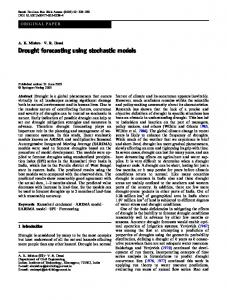
The amplitude of coherent oscillations in (2.2) increases as the control parameter λ → 0 and as the noise intensity δ increases, while the frequency is concentrated at a single value. The left column shows the time series for x(t) for δ1 = δ2 = δ. The right column shows the corresponding PSD. For both a) and b), the parameters in (2.2), α = −0.2, γ = −0.2, ω0 = 0.9, ω1 = 0, are the same. In (a) δ = .01, λ = −0.03 (solid line) and λ = −0.003 (dashed line). In (b) λ = −0.03, δ = 0.07 (solid line) and δ = 0.1 (dashed line). Recall λ = ǫ2 λ2 , measures distance from the Hopf point. . . . . . . The behavior of peak frequency from the PSD and the numerically computed coherence measure β are shown as functions of the noise. For all figures, the control parameter is λ = −0.03, the noise level is δ1 = δ2 = δ, and the other parameters in (2.2) are α = −0.2, γ = −0.2, and ω0 = 0.9. Upper: peak frequency ωp of the PSD peak vs. the noise intensity for ω1 = 0 in (a) ω1 = 1.2 in (c), and ω1 = −0.5 in (e). The solid line gives the asymptotic results (2.27) and the dotted line gives numerical results. Lower: coherence measure β vs. δ. The parameters in b),d), and f) match those in a),b), and c), respectively. . . . . . . . . . . . . . . . . . . . Time series for the subcritical case, taking α = 0.2, γ = −0.2, ω0 = 0.9, and ω1 = 1.2 in (2.2), with control parameter λ = −0.03. The noise levels are δ = 0.02 (bold line) and δ = 0.04 (thin line). Even though the noise levels for both are O(|λ|) = O(ǫ2 ), the variance of the amplitude for larger values of δ is sufficiently large to cause a transition to a state with O(1) oscillations . . . . . . . . . . . . . . . . . . . . . .

27

35

37

viii

2.4

3.1

3.2

Time series for diffusively coupled systems of the type (2.2) when the control parameter for each is λ = −0.03 and the other parameters are α = −0.2, γ = −0.2, ω0 = 2, ω1 = 1, starting with small initial conditions, illustrating different effects of the interaction of noise and coupling. Solid and dashed lines are for x(t) in the first and second oscillators, respectively, In Figures a) and b) the coupling strength is d = .05, while in Figure a) the noise levels are identical δ1 = 0.05, δ2 = 0.05 and in Figure b) the noise level of the first oscillator is reduced δ1 = 0.01, δ2 = 0.05. In Figure c) the noise levels are the same as in b), but the coupling is reduced, d = .001. . . . . . . . . . . . . . . . . . . . . . . . . The time series of the coupled ML model at different coupling strengths. gsyn = 0.15 mS/cm2 in (a) and 0.3 mS/cm2 in (b). The noise intensities are δ1 = δ2 = 0.7. Iapp = 97.5 µA/cm2 and vsyn = 70 mV . Other parameter values are given in Table B.1 in Appendix B. . . . . . . . . . . . . . . . . . . . . . . . . . . . . The bifurcation diagrams of a pair of ML neurons coupled through excitatory synapses in the absence of noise. vsyn = 70mV was used and four different coupling strengths are studied in (a)-(d). See Table B.1 in Appendix B for other parameter values. In (b)(d), the local bifurcation structure around the left(or right) SNB is illustrated in the left (or right) column. Stable SS and EAS are denoted by solid curves while all unstable states (steady and oscillatory) are represented by dashed lines. When stable AAS occurs, the LAOs and SAOs are marked with filled circles. Plus signs in (b) mark quasiperiodic solutions. HB points are marked by a filled square while the SNB points on oscillatory branches are denoted by filled diamonds. Limit points of the LAOs and SAOs are also SNBs which occur at an Iapp value very close to I0 , which are marked by open diamonds. Instability of LAOs and SAOs occur at a torus bifurcation (TR) points and are marked by open circles. (e) Time series of a typical AAS for Iapp = 97.5 µA/cm2 , gsyn = 0.15 mS/cm2 . Note that the phase difference between the two oscillations is 0.92 for the parameters values in Table B.1 in Appendix B. . . . . . . .

39

45

49

ix

3.3

3.4

3.5

The bifurcation diagrams of a pair of inhibitory ML neurons in absence of noise. vsyn = −75 mV and similar coupling strengths as in Fig. 3.2 were used here. The line types and the symbols have identical meanings as in Fig. 3.2. Note that for Iapp = 96.5 µA/cm2 and gsyn = 0.15 mS/cm2 in (b), AAS is the only stable oscillatory state. The time series of this solution is shown in (e). The time series of another AAS that coexists with the EAS at Iapp = 100 µA/cm2 is shown in (f). Beyond the TR point in (b), the only stable oscillatory state is the EAS. An example of this is shown in (g) for gsyn = 0.15 mS/cm2 . Other parameter values are given in Table B.1 in Appendix B. . . . . . . . . . . . . . . . . . . . . . . . . Bifurcation diagrams of diffusively-coupled λ − ω oscillators for five different coupling strengths (a)-(e). Stable solutions are plotted in solid lines while unstable solutions are represented by dashed lines. Different solution branches that are stable are marked by different letters. “A” marks the steady state branch, “B” for the EAS branch, “C” and “D” marks the LAO and the SAO of the AAS branch. Squares indicate HB points, diamonds indicate SNB points. Open circles represent TR points. Bifurcations in the two parameter space λ0 − ǫ are shown in (f). As defined in (a)-(e), the filled and open squares mark the two different HB points, the diamonds represent the SNB points and the open circles denote the TR points. The bold solid lines mark the approximate intervals where stable localized oscillations are obtained by using multi-scale analysis. The values of the other parameters are ω0 = 1, ω1 = 0.5, λ1 = 1. . . . . . . . . . . . . . . . . . . . . . . . . . . . . . Comparison between analytical and numerical results. Left panel: Bifurcation diagram of the coupled λ − ω system obtained using AUTO is plotted together with analytical approximation of the amplitudes of the LAOs and the SAOs (open diamonds). Right panel: phase difference between the two oscillators in the AAS as a function of λ0 . Solid line represents numerical results and open diamonds represent analytical approximations. The values of other parameters are ǫ = 0.02, ω0 = 1, λ1 = 1, ω1 = 0.5 . . . . . . . . .

51

54

56

x

3.6

The distributions of the phase difference ∆φ of excitatory neurons of (3.1)-(3.3) at different noise levels δ = δ1 = δ2 (δ = 0.4 for solid line; δ = 0.7 for dashed line and δ = 1.5 for dotted line) with Iapp = 97.5 µA/cm2 in (a)(c) and Iapp = 100.5 µA/cm2 in (b)(d). We take gsyn = 0.15 mS/cm2 and vsyn = 70 mV in (a)-(d) but use different thresholds: vth1 = 5 mV in the upper row and vth2 , slightly larger than veq in the range from −22 mV to −25 mV , in the lower row to detect both LAO and SAO. The histogram bin size in Figure 6-9 is 0.05. Other parameters are as listed in Table B.1. Recall that the phase difference of LAO and SAO is 0.92. . . . . . 3.7 The distributions of the phase difference ∆φ of excitatory neurons of (3.1)-(3.3) at different coupling strengths (gsyn = 0.15 mS/cm2 for solid line and gsyn = 0.3 mS/cm2 for dotted line) with Iapp = 97.5 µA/cm2 in (a)(c), Iapp = 100.5 µA/cm2 in (b)(d). We take the same noise intensities δi = 0.7 (i = 1, 2) and vsyn = 70 mV (excitatory case) in (a)-(d). Other parameters are as listed in Table B.1. As in the previous figure, we use a vth1 in the upper row, and vth2 in the lower row to detect both LAO and SAO. . . . . . . . . 3.8 The distributions of the phase difference ∆φ of excitatory neurons of (3.3) with gsyn = 0.15 mS/cm2 but different Iapp (Iapp = 235 µA/cm2 for solid line and 225 µA/cm2 for dashed line). In the simulation we take vth = 18 mV , to detect large spikes only. . . . 3.9 The distributions of the phase difference ∆φ of inhibitory ML neurons (3.1)-(3.3) at different regions. Upper row: different noise levels δ = δ1 = δ2 (δ = 0.4 for solid line; δ = 0.7 for dashed line and δ = 1 for dotted line) with gsyn = 0.15 mS/cm2 . Lower row: different coupling strengths gsyn = 0.15 mS/cm2 for solid line; gsyn = 0.3 mS/cm2 for dotted line with δ1 = δ2 = 0.7. We take Iapp = 96.5 in (a)(d), Iapp = 100 µA/cm2 in (b)(e) and Iapp = 101.5 µA/cm2 in (c)(f), and vsyn = −75 mV in (a)-(d). Other parameters are as listed in Table B.1. . . . . . . . . . . . 3.10 Synchrony diagram of 20 neurons in (3.17) with excitatory coupling strength gsyn = 0.8 mS/cm2 in (a)(e),0.5 in (b)(f), 0.3 in (c)(g), 0.15 in (d)(h) when Iapp = 96.5 in (a)-(d) and Iapp = 100.5 in (e)-(h). Other parameters are listed in Table B.1. . . . . . . . . .

58

59

60

62

63

xi

4.1

4.2

4.3

4.4

Bifurcation diagrams and the corresponding f −I relationship near a Case I (A) and a Case II (B) transition in theMorrisLecar (ML) model. Iapp is the control parameter. Stable and unstable equilibria are marked with solid and dashed lines respectively. Stable and unstable periodic solutions are marked with filled and open circles. The frequency of a steady state is calculated by using the eigenvalues of the corresponding linearized system. . . . . . . . . . . . . . . . . . . . . . . . . Spike-time reliability (STR) of the ML model in the Case I conditions (upper panels, (A)-(B)) and the Case II conditions (lower panels, (C)-(D)). Parameter values used are given in Table B.1. The standard deviation (SD) of the intrinsic noise is tuned to be 2 µA/cm2 for (A)-(B) 5 µA/cm2 for (C)-(D), and the SD of external noise is 5 µA/cm2 in (B) and 9 µA/cm2 in (D). . . . . . . . . . . . . . . . . . . . . . . . . . . . . . . Reliability R of the Case I (A) and Case II (C) ML models is plotted in the left columns against the SD of the external noise that is either convoluted (solid) or white (dashed). R is plotted against τ for the respective cases in the right columns. Parameter values are given in Table B.1. The SD of the intrinsic noise is tuned to be 2 µA/cm2 for (A) and (B) , and 5 µA/cm2 for (C) and (D). The SD of the external noise is 5 µA/cm2 in (B) and 9 µA/cm2 in (D). . . . . . . . . . . . . Spike triggered averages (STAs) for Case I (A) and Case II (C) ML models together with the corresponding response in membrane voltage. Artificial signals are generated (the upper panel in (B) and (D)) by connecting many copies of the STA with pieces of background fluctuations of different lengths that are known to be incapable of generating a spike. A typical response of a Case I (B) or a Case II (D) ML model to such a signal is shown in a raster plot. The SDs of the intrinsic and extrinsic noise are 2 µA/cm2 and 5 µA/cm2 in (A) and (B), and 5 µA/cm2 and 9 µA/cm2 in (C) and (D). The reliability measure R is calculated and marked in the figure for each case. . . . . . . . . . . . . . . . . . . . . . . . . . . .

75

76

78

80

xii

4.5

4.6

4.7

Reliability is insensitive to the frequency content of the noise signal when ISIs are long. Testing noise signals are generated by connecting distinct samples of spike-evoking epochs (SEEs) with intervals of samples that are known to be incapable of generating a spike. The power spectrum for each signal is plotted in the right panel. From top to bottom, the peak frequency component is located at 0.00641 kHz in (A), 0.004 kHz in (B), 0.01 kHz in (C), and is insignificant in (D). The values of R are calculated with data collected from 100 trials, each containing more than 45 spikes. . . . . . . . . . . Phase plane trajectories traced out by the responses of the model to two different SEEs (panels A and C) and the SEEs profiles (top) and the corresponding voltage responses (bottom) (panels B and D). Four time points A, B, C and D are chosen and the corresponding location of the pseudo slow manifolds (dashed lines) MA , MC and MD are plotted in (A) and (C). Dotted lines are nullclines when I = Iapp + Iext . . . Average energy in progressively shorter time intervals before the spike threshold is reached for both Case I (A) and Case II (D) ML models. The horizontal axis represent the duration of time over which energy is calculated, starting at the time when spiking threshold is reached. The shorter the time interval, the closer it is to the threshold. The thick solid curve represents the average energy of reliable SEEs and the thick dotted curves represent the upper and lower limits based on the SD. The thin solid curve denotes the average energy of unreliable SEEs and the thin dotted curves mark the upper and lower limits of the SD. The histogram of the values of the gating variable w when the reliable (bold line) and unreliable (thin line) spike trajectories pass the through threshold at vth = −20 mV are plotted in (B) and (D) for Case I and II models respectively. The thick solid curves are averages of 400 reliable SEEs and the thin solid curves are averages of 600 unreliable SEEs. . . . . . . . . . . . . . . . . . . . . . .

81

83

85

xiii

4.8

5.1

The distributions of energy values over a brief time interval of 20 ms for all reliable SEEs. Plotted in (A) and (D) are the energy distribution for Case I and Case II models, respectively. The distribution is equally divided into three subclasses. The STA of each subclass is shown in (B) and (E) with different line types each marking one subclass as in (A) and (D). The SD of spike times over all 40 trials for each SEE is calculated and the results are shown in (C) and (F). . . . . . . . . . . .

86

Three possible bifurcation structures (e.g. max/min(V ) v.s. Iapp ) with the corresponding parameter regimes marked between two vertical thin lines. . . . . . . . . . . . . . . . . . .

97

xiv

List of Abbreviations AAS CR CV EAS FHN FS HB HH IRP ISI LAO ML MMO ODE OU PSD RS SAO SD SDE SEE SNB SNIC SR SRM SS STA STR TR

Asymmetric amplitude state Coherence resonance Coefficient variance Equal amplitude state FitzHugh-Nagumo Fast spiking Hopf bifurcation Hodgkin-Huxley Interspike refractory period Inter spike interval Large amplitude oscillation Morris-Lecar Mixed-mode oscillation Ordinary differential equation Ornstein-Uhlenbeck Power spectrum density regular spiking Small amplitude oscillation standard deviation Stochastic differential equations Spike-evoking epoch Saddle node bifurcation Saddle node on an invariant cycle Stochastic resonance Spike response model Steady state Spike triggered average Spike time reliability Torus bifurcation

xv

Acknowledgements I would like to express my deepest gratitude to my super supervisors (in alphabetical order): Prof. Rachel Kuske and Prof. Yue-Xian Li for their invaluable suggestions and guidance, constant encouragement and patience during the course of this work. I wish to express my cordial appreciation to my supervisory committee members (in alphabetical order): Prof. Eric Cytrynbaum, Prof. Wayne Nagata, Prof. Anthony Peirce and Prof. Lawrence M. Ward for useful advice. I would like to thank Institute of Applied Mathematics and Department of Mathematics at UBC. Special thanks to Lee Yupitun, the graduate secretary and Marek Labecki, Research/IT Manager of IAM. Lastly, and most importantly, I wish to thank my parents, my husband, my daughter and my friends at UBC. Without your love and support, nothing would be possible.

xvi

Statement of Co-Authorship This thesis is a collaborative work with Rachel Kuske and Yue-Xian Li (in alphabetical order). The stochastic multi-scale method proposed in Section 1.3.1 and Chapter 2 of the present thesis was inspired by Rachel Kuske’s preliminary work on stochastic differential equations, and it was completed under the guidance of Rachel Kuske and Yue-Xian Li. The theoretical analysis in Section 3.3.2 is my work. I used MATLAB to perform the numerical computation except the bifurcation analysis that was produced using XPPAUT. XMGR was also used to plot almost all figures based on the numerical data generated by MATLAB and XPPAUT, and the rest was plotted in MATLAB. All the simulations and results in this thesis are my work and I am entirely responsible for any errors and inaccuracies. I wrote the first draft of each chapter. Chapters 1 and 5 were proofread by Rachel Kuske and Yue-Xian Li. Chapter 2 was revised by Rachel Kuske. Chapters 3 and 4 were revised by Yue-Xian Li.

xvii

Chapter 1

Introduction Noise is ubiquitously present in all natural systems. It occurs at almost any level of the nervous system [1]-[3] including stochastic fluctuations in gene expression [4], thermal noise existing almost everywhere, synaptic noise during the neurotransmitter release that further causes small perturbations of the receiving neuron’s membrane potential, random switches of ion channels between open and closed states and a fluctuating ion current as a result, and sensory noise. Often noise is seen as detrimental to the normal operation of a dynamical system. In the past three decades, however, experimental and theoretical studies have revealed that noise can play a constructive role to increase coherence or synchrony or reliability of neurons [5]-[9]. One of the well-known phenomena is termed stochastic resonance (SR), a phenomenon characterized by the existence of a non-zero noise level that optimizes the response of a dynamical system to a deterministic signal [10]-[15]. SR has been reported in various experimental contexts, such as detection of weak signals [16]-[17], mechanoreceptive hairs of crayfish [18]-[19], auditory hair cells of frogs [20], neocortical pyramidal neurons [21], human proprioceptive system [22]. SR has also been found to play a role in chemical reactions [23]-[27] and on ion channel transduction [28], in the feeding behavior of the paddlefish [29]-[31], in human brain waves [32], as well as in molecular sorting [33]. The effect of noise has attracted great interest from mathematicians, physicists and biologists due in part to the constructive role of noise. Whether noise is detrimental or constructive, the most important thing is to understand the source and effect of noise, that is, which type of noise it is and what role it plays. For instance, thermal noise has equal power throughout the frequency spectrum, which matches the property of white noise; as ion channels open and close randomly with a voltage-dependent rate, it can be modeled by a Poisson process. Both the thermal noise and ion channel noise are generated at the level of dynamics of individual neurons, so they are often called intrinsic noise. On the other hand, noise arising from synaptic transmission and network are called extrinsic noise. This thesis does not concern chaotic dynamics but one should note that 1

chaotic systems also appear to behave randomly. The combination of noise and complex nonlinear dynamics produces time series that are easily mistaken for deterministic chaos. If we believe that the random fluctuations are essential to the functioning of the systems, would other parts or characteristics of the systems, such as chaotic dynamics provide added function over stochastic fluctuations? There are no clear answers to this question. The present thesis focuses on the influence of noise in neuroscience, specifically three phenomena evoked by noise: coherence resonance (CR), stochastic synchrony and spike time reliability (STR). This work makes use of both a theoretical approach and computer simulations in order to understand the effects of noise on single neuron, weakly coupled neurons and the timing of the spike events. In Section 1.1 of this chapter, a short overview of the above three topics is provided. The specific objectives of our work are introduced in Section 1.2, accompanied by an outline of the structure of the thesis. Motivated by [34]-[36], in Section 1.3 a theoretical method to derive explicit stochastic amplitude and phase equations is proposed, combining Kuramoto’s method [34] and Ito’s formula [37]. This method is effective when the parameters are close to a critical point such as a Hopf bifurcation (HB). We also list the numerical methods used in this thesis in the second part of Section 1.4.

1.1 1.1.1

Overview Coherence Resonance

Coherence Resonance (CR) or autonomous stochastic coherence is characterized by the occurrence of coherent behaviors such as rhythmicity in the presence of an optimal level of noise in a system that is quiescent in a noisefree state [38]- [40]. The difference between CR and SR is that in CR noise itself (no other input signals) can induce coherence at an intermediate level. CR has been observed in a number of experimental studies such as electronic circuits [41]-[44], lasers diodes [45]-[49], semiconductor laser [50], excitable chemical reactions [51]-[59], the cat’s neural system [60], a neural pacemaker [61], a three electrode electrochemical cell [62], discharge plasmas close to a homoclinic bifurcation [63]. CR was also found in a number of numerical studies including the Feigenbaum map close to a period-doubling bifurcation [64], the Fitzhugh-Nagumo (FHN) model [65]-[66], the leaky integrate-andfire (LIF) model [67], the Hodgkin-Huxley (HH) model[68], the HindmarshRose (HR) model [69] and neural networks [70]-[73]. An excitable membrane patch size [74] or the system size of a circadian oscillator [75] can be selected 2

in order to maximize CR at an optimal level of intrinsic noise. CR occurs because noise can modify the dynamics of a deterministic system by shifting bifurcation points or inducing behaviors that have no deterministic counterpart [76]. In the study of CR, the parameters are chosen so that the system is quiescently located at a stable equilibrium state in the absence of noise. Thus, in an integrate-and-fire model, nonlinearity is hidden in the “firing threshold” and the “fire-and-reset” mechanism, although the model appears to be described by a system of linear ordinary differential equations (ODEs). Such a model can spike and even burst [61],[77] spontaneously when the state variable reaches a threshold at an appropriate choice of parameter values. A related fundamental question is how the noise influences the coherent frequency. Many numerical simulations of models exhibiting coherent resonance have shown an increasing frequency with the increase of the noise level [69, 71, 72, 78], and there are a few studies showing small changes on the resonant frequency [70]. We use a canonical model of a Hopf bifurcation to analyze the relationship between coherent frequency and noise intensity in [79]. The theoretical results indicate that, depending on the type of the model, the resonant frequency can increase, decrease or remain the same with the growth of the noise level. Studying the stochastic amplitude of coherent oscillators is another important aspect. Recently multiple scale techniques have been used to develop amplitude equations [35, 36, 79, 80]. [35] and [80] worked on the Van der Pol-Duffing oscillator subject to additive noise and/or multiplicative noise. [36] considered a delay differential equation close to a critical delay of a HB with both the additive and multiplicative noise. We employ the λ − ω system, a canonical model for a HB, at an excitable regime close to a HB driven by noise in [79]. In addition, the stochastic phase dynamics and the mechanism of coherence resonance are also discussed in [79] based on the analytical results. There are several options of measures to quantify the sensitivity of coherence to the noise. The coherence measure β, based on the power spectrum, is defined [38] as β = hp (∆ω/ωp )−1 , (1.1) where the power spectral density (PSD) has a peak at a frequency ωp with half-width ∆ω and height hp . Coefficient of variance (CV) Rp is defined [40] as p V ar tp (1.2) Rp = < tp > 3

where tp is the time interval between two consecutive pulses, also known as the interspike interval (ISIs). ISI is not a constant in stochastic dynamical systems. Correlation time measure τc can also be used [40] τc =

Z

∞

C 2 (t)dt, C(t) =

0

h˜ y (τ )˜ y (τ + t)i , y˜ = y − hyi h˜ y2 i

(1.3)

where y is one of the state variables of an oscillator and C(t) denotes the correlation time. As the figures of coherence versus noise intensity in [38] and [40] demonstrated, at an intermediate level of noise the coherence measures (1.1)-(1.3) reach a maximum and (1.2) has a minimum, which means that there is an optimal level of noise driving the most coherence behavior. Therefore, a combination of the above measures is recommended when studying noise-induced coherence.

1.1.2

Stochastic Synchrony

Synchrony refers to the process by which two or more nonlinear oscillators having the same frequency (or phase) or in an integer relationship of frequency [81]-[82], which is a potential coordinating mechanism for the neural activities. Therefore understanding synchronized activity of neurons is very important for the study of the brain. Our present understanding of synchrony in coupled oscillators is largely based on the phase theory of nonlinear oscillators. Simply speaking, the phase of an oscillator is the fraction of a complete cycle elapsed. One normally uses the phase definition based on the Hilbert transform. A signal s(t) can be written into an analytical signal: a(t) = s(t) + iu(t). u(t) is the Hilbert transform of s(t): R u(t) = π1 p.v. 0∞ s(τ )/(t − τ )dτ where p.v. represents the Cauchy principal value. The phase φ(t) of the signal s(t) is then defined as φ(t) = arctan

u(t) . s(t)

(1.4)

Another phase definition used frequently is based on ISIs: φ(t) = 2π

t − τk + 2π(k − 1) τk − τk−1

(1.5)

where τk is the time of the kth firing, τk − τk−1 is one of ISIs. Compared with (1.4), (1.5) only considers the firing times of a signal. Synchrony is normally measured by the phase difference of the oscillators. For example, a system consisting of two weakly coupled neurons is said to achieve a synchronous state, when the phase difference of the oscillators is 4

kept constant. If this constant is zero, we call it in-phase; if the constant is π, it is anti-phase. Neurons can be connected via excitatory and/or inhibitory synapses. In general both synapses can synchronize a deterministic neuronal network. An excitatory synapse often leads to a in-phase synchrony while an inhibitory synapse brings an anti-phase synchrony. Noise usually has a destructive effect on synchrony by inducing phase slips or shrinking the synchronization region [83]-[85]. On the other hand, synchrony can arise due to noise through SR or CR, or a canard mechanism of individual cells. There are a lot of experimental reports on how noisy currents facilitate synchronization, such as experimental observations in networks of circuits [87] and chemical reactions [88]-[90], in the crayfish caudal photoreceptor [91]-[92], in the cardiovascular and respiratory systems in healthy humans under free-running condition [93], in a paddlefish [94], in human perception and cognition [95], in the olfactory system [96], etc. In addition, many examples of numerical computation indicate the beneficial effect of noise on synchrony such as in the FHN model [66], in the HH model [68], in the HR model [69] and in a pacemaker [97]. In the stochastic systems, synchronization can be viewed using statistical tools. Normally, a peak presented in the histogram of the phase difference is regarded as an indicator of synchronization. The narrower the peak is, the better the synchrony is. However when a underlying deterministic system is complicate, for example the weakly coupled system with various solutions in Chapter 3 of the present thesis, phase difference does not have a very strong peak in its histogram and it tends to spread over the regime of [0, π] for larger level of noise because noise influences the system randomly visiting its different stable solutions and therefore phase difference slips very frequently. Stochastic synchrony can also be defined by the leading Lyapunov exponent. [98]-[99] showed that a synchrony is achieved in the presence of noise when the largest Lyapunov exponent of the phase equation is negative. Noise synchronizes the system by shifting the Lyapunov exponent to negative values. The cross-diffusion coefficient can also be used to measure stochastic synchronization in [65] for a network with more than two neurons. There phase difference Φ(t) is calculated by Φ(t, k) = φ(t, N/2) − φ(t, N/2 + k) where k = −N/2, ..., N/2. It is the phase difference of the oscillator in the middle and each oscillator. Hence the cross-diffusion coefficient of the ∗ kth oscillator Def f (k) and the synchrony measure of the network Def f are defined as Def f (k) =

1 1 d ∗ [hΦ2 (t, k)i − hΦ(t, k)i2 ], Def f = 2 dt N

N/2

X

Def f (k). (1.6)

k=−N/2

5

∗ Phase synchronization becomes stronger when Def f is lower.

1.1.3

Spike Time Reliability

A constant current applied to a neuron at different times usually triggers trains of spikes that do not show reliable timing due probably to the effects of intrinsic noise. A stochastically fluctuating signal, however, is capable of generating spikes with remarkably reliable spike timing [100]. This phenomenon has been referred to as spike time reliability (STR) [101]. STR has been observed in a sequence of in vitro and in vivo experiments and numerical studies [102]-[114] where various noise or input waveforms were used as the injected currents. It has been suggested that STR is a general property of neurons exhibiting spikes [115]. STR has drawn a great deal of attention because STR implies that noise can play a significant role in signal encoding and the spike timing is as important as the firing rate for the information transmission in the brain. Synchrony of uncoupled oscillators with common stochastic input can also be regarded as a special case of STR. [116] found that phase synchronization of bursts in noncoupled sensory neurons of paddlefish was induced by a common Ornstein-Uhlenbeck (OU) Gaussian noise. It is essentially a phenomenon of STR. The mechanism underlying STR is not completely understood yet. Researchers have investigated this problem from several aspects. [102]-[103] studied this problem in terms of a resonant effect, that is, reliability of spike timing is accomplished when the peak frequency of the current fluctuations (i.e. resonant frequency) is equal or close to the firing rate of the neuron (i.e. intrinsic frequency) in response to a constant stimuli that has the same value as the mean of the fluctuating current. Similarly, [104] found that intrinsic frequencies of neurons play an important role in STR according to their experiments on pyramidal cells and interneurons. [115] showed that, unlike periodic currents, the aperiodic currents above threshold induce the reliable timing of response and intrinsic noise does not accumulate over time. [105] focused on experimental and numerical studies of a neuronal pacemaker with bi-stability between quiescence and rhythmic firing. By averaging spike-triggered stimulus currents preceding spikes, they captured a specific waveform with a depolarizing-hyperpolarizing shape that reliably generates spikes. The effect of autocorrelation time of input signals was studied in [106], where neurons achieve a maximal STR when the autocorrelation time scale of the input fluctuations is located at an optimal level, for example in the range of a few milliseconds (2 − 5 ms) for mitral cells 6

and neocortical pyramidal cells. Because a phase-response curve (PRC) can characterize the time shift of spikes in a quadratic integrate-and-fire model, it was used to understand how small inputs influence spike times [117]. A mathematical analysis of two or more slightly different and uncoupled phase oscillators in [118] showed that, when the Lyapunov exponent is negative, reliability can be achieved when the common noise is small. Hence the sign of the Lyapunov exponent can also be a criteria to measure STR.

1.2

Objectives

Neurons can be treated as non-identical oscillators with weak connections to one another. For most of the neurons in the brain, they are often quiescent without input; and they are excitable, that is, they are able to generate action potentials when stimulated by an appropriate input. Therefore, in the noisy environment of the brain, neurons can exhibit coherent oscillators at an optimal level of noise. In Chapter 2, considering the above characteristics of neurons, we begin with the simplest case: a single quiescent oscillator that exhibits coherent oscillations subject to noise. We investigate the behavior of a nonlinear quiescent oscillator, especially its phase and amplitude dynamics under the influence of noise. We use the normal form of HB as our first model. The control parameter is chosen to be outside of the HB in order to satisfy the expected characteristics. A stochastic multi-scale method is developed to derive stochastic amplitude and phase equations. The analytical method is proven to be effective by a comparison of analytical and numerical results. In addition, based on the analytical results, the relationship between coherent frequency and noise intensity, and the reasons why a maximum coherence occur at an optimal noise level are discussed in Chapter 2. The second topic of this thesis covered in Chapter 3 is to understand stochastic synchrony, which is associated with the fact that neurons communicate with one another in real life. In order to complete a simple action, such as drinking or walking, information in the form of electrochemical currents from other neurons is transmitted to a neuron via synapses (e.g. excitatory and/or inhibitory). Thus an action potential or a burst of that neuron is generated, and then it is sent to other neurons. Through phase locking of action potentials (i.e. synchronization), information is transmitted robustly in the brain full of noise. The presence of SR and/or CR can help the neurons to achieve synchrony. The influence of the coupling on phase dynamics in deterministic systems has been studied extensively in 7

[34], [119]-[122]. The presence of noise, however, challenges the deterministic theory of weakly coupled oscillators. Therefore, the second objective of this thesis to be discussed in length in Chapter 3, is to understand the phase dynamics of weakly coupled oscillators driven by noise. We use a simple case of two identical neurons where each of them is represented by a Morris-Lecar (ML) [123] model that was developed in the study of the excitability of the barnacle giant muscle fiber. They are weakly connected through synaptic coupling. The parameter regime between a subcritical HB point and a saddle node bifurcation (SNB) point of the periodic branch that bifurcates from the HB point is considered. Surprisingly, the bifurcation analysis of the deterministic system illustrates a multi-stability of fixed points, symmetric superthreshold oscillations, and asymmetric localized oscillations. Then two independent Brownian Motions are applied to each neuron respectively as additive noise and the phase interactions of weakly coupled oscillators are studied in the presence of noise. The interaction of noise and various coexisting oscillations induces a complex behavior known as mixed-mode oscillations (MMOs). The detailed reason why MMOs occur and their consequent influence on synchrony in such a weakly coupled neuronal system are discussed in Chapter 3. The time location of spikes (or the firing timing) is closely correlated with synchrony. It is reported that fluctuating input signals may carry information from other neurons. Hence understanding spike timing contributes greatly to our understanding of the communication in the brain. Our investigation of the mechanism of STR is presented in Chapter 4. Neurons has two basic cases of excitability, often referred to as Case I and Case II. As quiescence-to-oscillation transition occurs, the oscillation frequency of Case I neurons gradually increases from zero, however the frequency jumps to a nonzero value at the transition point in Case II. Both cases are considered in this study. We are interested in the excitable parameter regime. In the Case I model this regime is close to a saddle node on an invariant cycle (SNIC), and in the Case II model it close to a SNB on the period branch arising from a subcritical HB. We construct artificial signals with different frequency components and apply them into our model. The spike trains achieve good reliability for each artificial signal, even for a broad-band frequency signal. This result is in contrast with the resonant effect mechanism in which resonant frequency causes more reliable spike times in a firing regime as stated in Section 1.1.3. The phase plane analysis of our model indicates that the threshold of voltage responses changes with fluctuation, which is consistent with in vivo experiments in [124]-[125] where the threshold is found to be 8

variable with the random opening of N a+ channels. Finally we present an explanation in terms of the “energy” for STR.

1.3 1.3.1

Methods Analytical Method

The purpose of this section is to develop an analytical method to understand the resonant effects of noise in an excitable system in the neighborhood of a HB. The aim of this method is to derive explicit expressions for amplitude and phase in terms of parameters of deterministic systems and noise terms so that the influence of the system and noise on the resonant behaviors can be quantitatively evaluated. Kuramoto provided a classic scheme to derive a small amplitude solution of a deterministic system in the vicinity of a HB point in [34]. Inspired by recent work in [35]-[36], we expand Kuramoto’s approach to the field of stochastic differential equations (SDEs) using Ito’s formula and the properties of white noise [37]. Let’s start from a general system of stochastic differential equation: dX = F (X; µ)dt + δdW (t),

(1.7)

Here X, F , δ and W are n−dimensional vectors. µ is a real parameter and µ = µ0 = 0 corresponds to a Hopf bifurcation point. δi are noise levels, and dWi (t) are independent standard Brownian white noise. The deterministic version of (1.7) has a stable steady state X0 , i.e. F (X0 ) = 0. We follow the approach in [34] to treat the deterministic part of the right hand side of (1.7), expressed in terms of V = X − X0 in a Taylor series: (Use this as a heuristic for demonstration purpose only; in general one would need to use Ito’s formula) dX = [F (X0 ) + LV + M V V + N V V V + ...]dt + δdW (t),

(1.8)

where L is the Jacobian matrix of F , and M V V and N V V V are vectors defined by (M V V )i =

X 1 ∂ 2 Fi (X0 ) m,l

2 ∂X0i X0j

Vm Vl , (N V V V )i =

∂ 3Fi (X0 ) Vm Vl Vk . 6 ∂X0i X0j X0k

X 1

m,l,k

Near a Hopf bifurcation, L, M and N maybe developed in powers of ǫ: ℓ = l0 + χǫ2 ℓ1 + ǫ4 ℓ2 , ℓ = L, M, N.

(1.9) 9

ǫ is a small positive number, ǫ2 = χµ. χ = sgn(µ) = −1 because we are interested in the effect of noise on the stable steady state X0 . L0 is the Jacobian matrix of F at a Hopf bifurcation. The eigenvalues corresponding to L is denoted as λ ± iω0 , and λ ∼ O(ǫ2 ), so we take λ = ǫ2 Λ, Λ ∼ O(1). λ = 0 when µ = 0 at a Hopf bifurcation point, and λ < 0 when µ < 0. We are looking for an approximation of X like X = X0 + ǫU1 + ǫ2 U2 + O(ǫ3 ),

(1.10)

Assume that all components of n, to the leading order, are oscillators with frequency ω, so (1.10) can actually be expressed as X = X0 + ǫ[A(T ) cos ωt + B(T ) sin ωt] +ǫ2 [C(T ) cos 2ωt + D(T ) sin 2ωt + E(T )] + O(ǫ3 ),

(1.11)

where T = ǫ2 t is the slow time scale, which is appropriate with the fact that the amplitude of the oscillators varies slowly with noise; t and T should be treated as mutually independent, dT = ǫ2 dt. A(T ),..., and E(T ) are stochastic vectors on the slow time scale measuring the effect of noise on the stable solution, C,..., and E are functions of A and B. We restrict our analysis to the case that ǫ ≪ 1 and δi ≪ 1 such that µ is in the vicinity of Hopf bifurcation and the noise is weak.vectors with constant elements A good approximation for the equations for A(T ) and B(T ) can be written as the combination of drift term and diffusion terms: dAi = ϕAi dT + σAi dξAi (T ), dBi = ϕBi dT + σBi dξBi (T ),

(1.12)

where ξli (l = A, B; i = 1, ..., n) are independent standard Brownian motions. Among the diffusion terms, σli dξli represent the contributions coming from the noise terms δdW in (1.7) to l = A, B. The drift coefficients ϕli and noise intensity σli (l = A, B; i = 1, ..., n) are unknown and may depend on A and B. The detailed discussion of (1.12) is presented in [36]. The substitution of (1.11) and (1.9) into (1.8) gives dX = [ǫ(L0 U1 ) + ǫ2 (L0 U2 + M0 U1 U1 ) + ǫ3 (L0 U3 − L1 U1 + 2M0 U1 U2 +N0 U1 U1 U1 )]dt + δdW (t)

(1.13)

The left hand side of (1.7) could be transformed using Ito’s formula [37], which is the “chain rule” for stochastic functions. Furthermore X, dA and dB are substituted with (1.11) and (1.12), which gives dXi =

X σ 2 ∂ 2 Xi ∂Xi ∂Xi ∂Xi k dt + dAi + dBi + dT + ...(1.14) ∂t ∂Ai ∂Bi 2 ∂k2 k=A ,B i

i

10

σ2

2

where k=Ai ,Bi 2k ∂∂kX2i dT would give higher order corrections for δ < ǫ. Furthermore X, dA and dB in (1.14) are substituted with (1.11) and (1.12), which gives P

dXi = [ǫ(−Ai ω sin ωt + Bi ω cos ωt) + ǫ2 (−2Ci ω sin ωt + 2Di ω cos ωt) +ǫ3 (ϕAi cos ωt + ϕBi sin ωt) + O(ǫ4 )]dt

+ǫ[cos ωtσAi dξAi (T ) + sin ωtσBi dξBi (T )]

(1.15)

Equating coefficients of different powers of ǫ of drift terms in (1.13) and (1.15), we get a set of equations. At the order of ǫ, (L0 U1 )i = −Ai ω sin ωt + Bi ω cos ωt,

(1.16)

which leads to ω = ω0 for all ω in (1.13) and (1.15). At the order of ǫ2 , we have (L0 U2 )i + (M0 U1 U1 )i = −2Ci ω0 sin 2ω0 t + 2Di ω0 cos 2ω0 t.

(1.17)

At the order of ǫ3 , we have (L0 U3 )i − (L1 U1 )i + 2(M0 U1 U2 )i + (N0 U1 U1 U1 )i

= ϕAi cos ω0 t + ϕBi sin ω0 t.

(1.18)

In order to get equations of ϕAi and ϕBi ), we use a projection similar to the solvability condition for deterministic systems on (1.18): Z

0

2π ω0

∗

a cos ω0 t(1.18)dt = 0,

Z

2π ω0

0

b∗ sin ω0 t(1.18)dt = 0,

(1.19)

Here a∗ and b∗ are eigenvectors for the adjoint matrix L∗0 of Jacobian matrix L0 , and a∗ a = 1, b∗ b = 1. The expressions of ϕA and ϕB can be obtained ϕA = ΛA + a∗ f (A, B), ϕB = ΛB + b∗ g(A, B),

(1.20)

where f (A, B) and g(A, B) are nonlinear functions related to cos ω0 t and sin ω0 t. Equating diffusion terms in (1.13) and (1.15), we get ǫ[cos ω0 tσAi dξAi (T ) + sin ω0 tσBi dξBi (T )] = δi dWi (t).

(1.21)

With the following property of noise [37], dWi = cos ω0 tdη1i (t) + sin ω0 tdη2i (t) =

1 (cos ω0 tdη1i (T ) + sin ω0 tdη2i (T )), ǫ 11

where i = 1, ..., n. (1.21) is developed as cos ω0 t[ǫ2 σAi dξAi (T ) − δi dη1 (T )] + sin ω0 t[ǫ2 σBi dξBi (T ) − δi dη2 (T )] = 0, (1.22) Using the same projection as (1.19) and making ξAi (T ) = η1i (T ) and ξBi (T ) = η2i (T ), we derive the following: σAi =

δi δi , σBi = 2 , i = 1, ..., n. 2 ǫ ǫ

(1.23)

So the A, B equations are obtained by substituting (1.20) and (1.23) into (1.12); the expressions of C(T ), D(T ) and E(T ) as quadratic functions of A(T ) and B(T ) can be derived by applying the projection (1.19) on (1.17). Further the equation of X will be derived through (1.11).

1.3.2

Numerical Methods

The stochastic differential equations in this thesis are simulated using the Euler-Maruyama Method to incorporate with stochastic terms. A stochastic differential equation given by dx = f (x, t)dt + δdw with initial condition x(0) = x0 can be solved numerically with the following step √ xk+1 = xk + hf (xk ) + hδw(k). Here h is the step size, equaling a time interval of period divided by around 200 sampling points. w(k) is generated by a random number generator of MATLAB with mean 0 and standard deviation 1. The bifurcation diagrams plotted in the thesis are calculated using XPPAUT [126], which is a useful mathematical package for exploring phase spaces and dynamical systems.

12

Bibliography [1] S. F. Traynelisa and F. Jaramilloa, Getting the most out of noise in the central nervous system, Trends in Neurosciences, 21 (1998) 137-145. [2] A. Manwani, and C. Koch, Detecting and estimating signals in noisy cable strucures I: Neuronal noise sources. Neural Comput., 11 (1999) 1797-1829. [3] A. Aldo Faisal, Luc P.J. selen and Daniel M. Wolpert, Noise in the nervous system, Nature Reviews Neuroscience, 9 (2008) 292-303. [4] P. S. Swain, M. B. Elowitz, and E. D. Siggia, Intrinsic and extrinsic contributions to stochasticity in gene expression, Proc. Natl. Acad. Sci. U.S.A. 99 (2002) 12795. [5] A. Bulsara, P. Hanggi, F. Marchesoni, F. Moss and M. Shlesinger, eds, Stochastic Resonance in Physics and Biology, J. Stat. Phys. 70 (1993) 1-512. [6] A Longtin, Stochastic resonance in neuron models. J. Stat. Phys. 70 (1993) 309. [7] K. Wiesenfeld, F. Moss, Stochastic resonance and the benefits of noise: from ice ages to crayfish and SQUIDs, Nature 373 (1995) 33-36. [8] F. Moss F, L.W. Ward, W.G. Sannita, Stochastic resonance and sensory information processing: a tutorial and review of application, Clin Neurophysiol, 115 (2004) 267-281. [9] B. Lindner, J. Garcia-Ojalvo, A. Neiman, and L. Schimansky-Geier, Effects of noise in excitable systems. Phys. Rep. 392 (2004) 321. [10] R. Benzi, A. Sutera and A. Vulpiani, The mechanism of stochastic resonance, J. Phys., 14 (1981) 453-457. [11] R. Benzi, G. Parisi, A. Sutera and A. Vulpiani, Stochastic resonance in climate change, Tellus, 34 (1982) 10-16. 13

[12] C. Nicolis, Solar variability and stochastic effects on climate, Sol. Phys. 74 (1981) 473-478. [13] C. Nicolis, Stochastic aspects of climatic transitions-response to a periodic forcing, Tellus 34 (1982) 1-9. [14] B. McNamara, K. Wiesenfeld, and R. Roy, Observation of Stochastic Resonance in a Ring Laser, Phys. Rev. Lett. 60 (1988) 2626-2629. [15] B. McNamara, K. Wiesenfeld, Theory of stochastic resonance, Phys. Rev. A 39 (1989) 4854-4869. [16] P. Jung and P. Hanggi, Amplification of small signals via Stochastic Resonance, Phys. Rev. A, 44 (1991) 8032-8042. [17] P. Hanggi, Stochastic Resonance in Biology How Noise Can Enhance Detection of Weak Signals and Help Improve Biological Information Processing, Chemphyschem, 3 (2002) 285-290. [18] J.K. Douglass, L. Wilkens, E. Pantazelou, F. Moss, Noise enhancement of information transfer in crayfish mechanoreceptors by stochastic resonance, Nature, 365 (1993) 337-340. [19] S. Bahar, A. Neiman, L.A. Wilkens, F. Moss, Phase synchronization and stochastic resonance effects in the crayfish caudal photoreceptor, Phys. Rev. E, 65 (2002) R050901-R050904. [20] F. Jaramillo, K. Wiesenfeld, Mechanoelectrical transduction assisted by Brownian motion: a role for noise in the auditory system, Nat. Neurosci., 1 (1998) 384-388. [21] M. Rudolph, A. Destexhe, Do Neocortical Pyramidal Neurons Display Stochastic Resonance? J. Comput. Neurosci., 11 (2001) 19-24. [22] P. Cordo, J.T. Inglis, S. Verschueren, J.J. Collins, D.M. Merfeld, S. Rosenblum, S. Buckley, and F. Moss, Noise in human muscle spindles, Nature, 383 (1996) 769-770. [23] A. Guderian, G. Dechert, K.P. Zeyer, F.W. Schneider, Stochastic Resonance in Chemistry -1I. The Belousov-Zhabotinsky Reaction, J. Phys. Chem., 100 (1996) 4437-4441. [24] A. Forster, M. Merget, F.W. Schneider,Stochastic Resonance in Chemistry - 2. The Peroxidase-Oxidase Reaction, J. Phys. Chem., 100 (1996) 4442-4447. 14

[25] W. Hohmann, J. Muller, F.W. Schneider, Stochastic Resonance in Chemistry - 3. The Minimal Bromate Reaction, J. Phys. Chem., 100 (1996) 5388-5392. [26] T. Ameniya, T. Ohmori, M. Nakaiwa, T. Yamguchi, Two-Parameter Stochastic Resonance in a Model of the Photosensitive BelousovZhabotinsky Reaction in a Flow System, J. Phys. Chem. A, 102 (1998) 4537-4542. [27] T. Ameniya, T. Ohmori, T. Yamamoto, T. Yamguchi, Stochastic Resonance under Two-Parameter Modulation in a Chemical Model System, J. Phys. Chem A, 103 (1999) 3451-3454. [28] S.M. Bezrukov, I. Vodyanoy, Noise-induced enhancement of signal transduction across voltage-dependent ion channels, Nature, 378 (1995) 362. [29] D.F. Russell, L.A. Wilkens, F. Moss, Use of behavioural stochastic resonance by paddlefish for feeding, Nature, 402 (1999) 291-294. [30] J.A. Freund, J. Kienert, L. Schimansky-Geier, B. Beisner, A. Neiman, D.F. Russell, T. Yakusheva, F. Moss, Behavioral stochastic resonance: How a noisy army betrays its outpost, Phys. Rev. E, 63 (2001) 031910. [31] D.F. Russell, A. Tucker, B.A. Wettring, A. Neiman, L. Wilkens, and F. Moss, Noise effects on the electrosense-mediated feeding behavior of small paddlefish, Fluctuation Noise Lett., 2 (2001) L71-L86. [32] T. Mori and S. Kai, Noise-induced entrainment and stochastic resonance in human brain waves, Phy. Rev. Letters, 88 (2002) 218101. [33] D. Alcor, V. Croquette, L. Jullien and A. Lemarchand, Molecular sorting by stochastic resonance, Proc. Nat. Acad. Sci. U.S.A. 101 (2004) 8276-8280. [34] Y. Kuramoto, Chemical Oscillations, Waves and Turbulence (Springer, Berlin, 1984). [35] R. Kuske, Multi-scale analysis of noise-sensitivity near a bifurcation, IUTAM Conference: Nonlinear Stochastic Dynamics, (2003) 147-156. [36] M. M. Klosek and R. Kuske, Multiscale Analysis of Stochastic Delay Differential Equations, SIAM Multiscale Model. Simul., 3 (2005) 706729. 15

[37] Z. Schuss, Theory and applications of stochastic differential equationss (Wiley, New York, 1980). [38] G. Hu, T. Ditzinger, C.-Z. Ning, H. Haken, Stochastic resonance without. external periodic force, Phys. Rev. Lett. 71 (1993) 807-810. [39] W.J. Rappel, S.H. Strogatz, Stochastic resonance in an autonomous system with a nonuniform limit cycle, Phys. Rev. E, 50 (1994) 32493250. [40] A.S. Pikovsky, J. Kurths, Coherence resonance in a noise-driven excitable system, Phys. Rev. Lett., 78 (1997) 775-778. [41] D.E. Postnov, S.K. Han, T.G. Yim, O.V. Sosnovtseva, Experimental observation of coherence resonance in cascaded excitable systems, Phys. Rev. E, 59 (1999) R3791-R3794. [42] Y. Horikawa, Coherence resonance with multiple peaks in a coupled FitzHugh-Nagumo model, Phys. Rev. E, 64 (2001) 031905-031910. [43] D.E. Postnov, O.V. Sosnovtseva, S.K. Han, W.S. Kim, Noise-induced multimode behavior in excitable systems, Phys. Rev. E, 66 (2002) 016203-016207. [44] I.Z. Kiss, J.L. Hudson, G.J. Escalera Santos, P. Parmananda, Experiments on coherence resonance: Noisy precursors to Hopf bifurcations, Phys. Rev. E, 67 (2003) 035201-035204. [45] G. Giacomelli, M. Giudici, S. Balle, J.R. Tredicce, Experimental Evidence of Coherence Resonance in an Optical System, Phys. Rev. Lett. 84 (2000) 3298-3301. [46] S. Barbay, G. Giacomelli, F. Marin, Experimental Evidence of Binary Aperiodic Stochastic Resonance, Phys. Rev. Lett. , 85 (2000) 4652-4655. [47] F. Marino, M. Giudici, S. Barland, S. Balle, Experimental Evidence of Stochastic Resonance in an Excitable Optical System, Phys. Rev. Lett. 88 (2002) 040601-040604. [48] A.M. Yacomotti, G.B. Mindlin, M. Giudici, S. Balle, S. Barland, J. Tredicce,Coupled optical excitable cells, Phys. Rev. E, 66 (2002) 036227-036237.

16

[49] J.F. Martinez Avila, H.L. de S Cavalcante, J.R. Leite, Experimental Deterministic Coherence Resonance, Phys. Rev. Lett., 93 (2004) 144101144104. [50] O. V. Ushakov, H.J. Wnsche, F. Henneberger, I. A. Khovanov, L. Schimansky-Geier, and M. A. Zaks, Coherence Resonance Near a Hopf Bifurcation, Phys. Rev. Lett. 95, (2005) 123903-123907. [51] Z. Hou, H. Xin, Enhancement of Internal Signal Stochastic Resonance by Noise Modulation in the CSTR System, J. Phys. Chem. A, 103 (1999) 6181-6183. [52] S. Zhong, H. Xin, Internal Signal Stochastic Resonance in a Modified Flow Oregonator Model Driven by Colored Noise, J. Phys. Chem. A, 104 (2000) 297-300. [53] Y. Jiang, Shi Zhong, H. Xin, Experimental Observation of Internal Signal Stochastic Resonance in the Belousov-Zhabotinsky Reaction, J. Phys. Chem. A, 104 (2000) 8521-8523. [54] Q.S. Li, R. Zhu, Stochastic resonance with explicit internal signal, J. Chem. Phys. 115 (2001) 6590-6595. [55] K. Miyakawa, H. Isikawa, Experimental observation of coherence resonance in an excitable chemical reaction system, Phys. Rev. E, 66 (2002) 046204-046207. [56] K. Miyakawa, T. Tanaka, H. Isikawa, Dynamics of a stochastic oscillator in an excitable chemical reaction system, Phys. Rev. E, 67 (2003) 066206-066209. [57] S. Zhong, H.W. Xin, Effects of colored noise on internal stochastic resonance in a chemical model system, Chem. Phys. Lett. 333 (2001) 133-138. [58] L.Q. Zhou, X. Jia, Q. Ouyang, Experimental and Numerical Studies of Noise-Induced Coherent Patterns in a Subexcitable System, Phys. Rev. Lett., 88 (2002) 138301-138304. [59] V. Beato, I. Sendina-Nadal, I. Gerdes, H. Engel, Coherence resonance in a chemical excitable system driven by coloured noise. Philos Transact A Math Phys Eng Sci., 366 (2007) 381-395.

17

[60] E. Manjarrez, J.G. Rojas-Piloni, I. Mendez, L. Martnez, D. Velez, D.Vquez, A. Flore, Internal stochastic resonance in the coherence between spinal and cortical neuronal ensembles in the cat, Neurosci. Lett. 326 (2002) 93-96. [61] H. Gu, M. Yang, L. Li, Z. Liu, W. Ren, Experimental observation of the stochastic bursting caused by coherence resonance in a neural pacemaker, Neuroreport, 13 (2002) 1657-1660. [62] M. Rivera, Gerardo J. Escalera Santos, J. Uruchurtu-Chavar, and P. Parmananda, Intrinsic coherence resonance in an electrochemical cell, Phys. Rev. E, 72 (2005) 030102-0300105. [63] Md. Nurujjaman, A. N. Sekar Iyengar, and P. Parmananda, Noiseinvoked resonances near a homoclinic bifurcation in the glow discharge plasma, Phys. Rev. E, 78 (2008) 026406. [64] A. Neiman, P.I. Saparin, L. Stone, Coherence resonance at noisy precursors of bifurcations in nonlinear dynamical systems. Physical Review E, 56 (1997) 270-273. [65] A. Neiman, L. Schimansky-Geier, A. Cornell-Bell, F. Moss, NoiseEnhanced Phase Synchronization in Excitable Media, Phys. Rev. Lett., 83 (1999) 4896-4899. [66] K. Nagai, H. Nakao,Y. Tsubo, Synchrony of neural Oscillators induced by random telegraphic currents, Phys. Rev. E, 71 (2005) 036217-036224. [67] K. Pakdaman, S. Tanabe, T. Shimokawa, Coherence resonance and discharge time reliability in neurons and neuronal models. Neural Netw, 14 (2001) 895-905. [68] C.S. Zhou, J. Kurths, Noise-induced synchronization and coherence resonance of a. Hodgkin- Huxley model of thermally sensitive neurons, Chaos, 13 (2003) 401. [69] S. Reinker, Y.-X. Li, R. Kuske Noise-Induced Coherence and Network Oscillations in a Reduced Bursting Model, Bulletin of Mathematical Biology, 68 (2006) 1401. [70] W.J. Rappel, A. Karma, Noise-Induced Coherence in Neural Networks, Phys.Rev. Lett., 77 (1996) 3256-3259.

18

[71] Y. Wang, D.T.W. Chik, Z.D. Wang, Coherence resonance and noiseinduced synchronization in globally coupled Hodgkin-Huxley neurons, Phys. Rev. E, 61 (2000) 740-746. [72] M. Zhan, G. W. Wei, C.H. Lai, Y.C. Lai, and Z. Liu, Coherence resonance near the Hopf bifurcation in coupled chaotic oscillators, Phys. Rev. E, 66 (2002) 036201. [73] D. Chik and A. Coster, Noise accelerates synchronization of coupled nonlinear oscillators, Physical Review E, 74 (2006) 041128. [74] G. Schmid, and P. Hanggi, Intrinsic coherence resonance in excitable membrane patches, Mathematical Biosciences, 207 (2007) 235-245. [75] M. Yi, Ya Jia, Q. Liu, J. Li, and C. Zhu, Enhancement of internalnoise coherence resonance by modulation of external noise in a circadian oscillator, Phys. Rev. E, 73 (2006) 041923-041930. [76] W. Horsthemke, R. Lefever, stochastic Transitions, (Springer Series in Synergetics, 2006). [77] A. Longtin, Autonomous stochastic resonance in bursting neurons. Phys. Rev. E. 55 (1997) 868-876. [78] T. Ditzinger, C. Z. Ning, and G. Hu, Resonancelike responses of autonomous nonlinear systems to white noise, Phys. Rev. E, 50 (1994) 3508-3516. [79] Na Yu, R. Kuske, and Y. X. Li , Stochastic phase dynamics: Multiscale behavior and coherence measures, Physical Review E, 73 (2006) 056205. [80] C. Mayol, R. Toral, and C. R. Mirasso, Derivation of amplitude equations for nonlinear oscillators subject to arbitrary forcing, Phys. Rev. E, 69 (2004) 066141. [81] A. Pikovsky, M. Rosenblum, and J. Kurths, Synchronization: A Universal Concept in Nonlinear Sciences, (Cambridge: Cambridge University Press, 2001) . [82] S. H. Strogatz and I. Stewart. Coupled oscillators and biological synchronization. Scientific American, 269 (1993) 102-109. [83] R.L. Stratonovich, Topics in the Theory of Random Noise, (Gordon and Breach, New York, 1967). 19

[84] P. Tass, M. G. Rosenblum, J. Weule, J. Kurths, A. Pikovsky, J. Volkmann, A. Schnitzler, and H.-J. Freund, Detection of n:m Phase Locking from Noisy Data: Application to Magnetoencephalography, Phys. Rev. Lett., 81 (1998) 3291-3294. [85] L.Q. Zhu, A. Raghu, Y.C. Lai, Experimental Observation of Superpersistent Chaotic Transients, Phys. Rev. Lett. 86 (2001) 4017-4020. [86] J. Drover, J. Rubin, J. Su, B. Ermentrout, Analysis of a Canard Mechanism by Which Excitatory Synaptic Coupling Can Synchronize Neurons at low firing frequencies SIAM Journal on Applied Mathematics, 65 (2004) 69-92. [87] S.K. Han, T.G. Yim, D.E. Postnov, O.V. Sosnovtseva, Interacting Coherence Resonance Oscillators, Phys. Rev. Lett. 83 (1999) 1771-1774. [88] S. Zhong, H. Xin, Effects of Noise and Coupling on the Spatiotemporal Dynamics in a Linear Array of Coupled Chemical Reactors, J. Phys. Chem. A, 105 (2001) 410-415. [89] C.S. Zhou, J. Kurths, I.Z. Kiss, J.L. Hudson, Noise-Enhanced Phase Synchronization of Chaotic Oscillators, Phys. Rev. Lett. 89 (2002) 014101-014104. [90] K. Miyakawa, H. Isikawa, Noise-enhanced phase locking in a chemical oscillator system, Phys. Rev. E, 65 (2002) 056206-056210. [91] S. Bahar, F. Moss, Stochastic phase synchronization in the crayfish mechanoreceptor/photoreceptor system, Chaos, 13 (2003) 138-144. [92] S. Bahar, and F. Moss, Stochastic resonance and synchronization in the crayfish caudal photoreceptor, Mathematical Biosciences 188 (2004) 8197. [93] C. Schafer, M.G. Rosenblum, H.-H. Abel, and J. Kurths, Synchronization in the human cardiorespiratory system, Phys. Rev. E, 60 (1999) 857-870. [94] A. Neiman, X. Pei, D. Russell, W. Wojtenek, L. Wilkens, F. Moss, H.A. Braun, M.T. Huber, and K. Voigt, Synchronization of the electrosensitive cells in the paddlefish, Phys. Rev. Lett. 82 (1999) 660-663. [95] L.M. Ward, S.M. Doesburg, K. Kitajo, S.E. MacLean, A.B. Roggeveen, Neural synchrony in stochastic resonance, attention, and consciousness, 20

Current issue feedCanadian Journal of Experimental Psychology, 60 (2006) 319-326. [96] S. Lagier, A. Carleton, and P.M. Lledo, Interplay between Local GABAergic Interneurons and Relay Neurons Generates γ Oscillations in the Rat Olfactory Bulb, The Journal of Neuroscience, 24 (2004) 4382-4392. [97] M. Perc, and M. Marhl, Pacemaker enhanced noise-induced synchrony in cellular arrays, Physics Letters A, 353 (2006) 372-377. [98] J. Teramae and D. Tanaka, Robustness of the Noise-Induced Phase Synchronization in a General Class of Limit Cycle Oscillators, Phys. Rev. Lett. 53 (2004) 204103-204106. [99] D.S. Goldobin and A. Pikovsky, Antireliability of noise-driven neurons, Physica A, 351 (2005) 061906-061909. [100] H.L. Bryant and J.P. Segundo, Spike initiation by transmembrane current: a white-noise analysis. J Physiol., 260 (1976) 279C314. [101] Z.F. Mainen and T.J. Sejnowski, Reliability of spike timing in neocortical neurons, Science, 268 (1995) 1503-1506. [102] J.D. Hunter, J.G. Milton, P.J. Thomas, and J.D. Cowan, Resonance Effect for Neural Spike Time Reliability, J. Neurophysiol. 80 (1998) 1427-1438. [103] J.D. Hunter and J. G. Milton, Amplitude and Frequency Dependence of Spike Timing: Implications for Dynamic Regulation, J. Neurophysiol., 90 (2003) 387-394. [104] J.M. Fellous, A.R. Houweling, R.H. Modi, R.P.N. Rao, P.H.E. Tiesinga, and T.J. Sejnowski, Frequency dependence of spike timing reliability in cortical pyramidal cells and interneurons, J. Neurophysiol, 85 (2001) 1782-1787. [105] D. Paydarfar, D.B. Forger, J.R. Clay, Noisy inputs and the induction of on-off switching behavior in a neuronal pacemaker, J Neurophysiol., 96 (2006) 3338-3348. [106] R.F. Galan, G.B. Ermentrout, and N. N. Urban, Optimal time scale for spike-time reliability: Theory, simulations and experiments, J Neurophysiol, 99 (2008) 277-283. 21

[107] T. Tateno and H.P.C. Robinson, Rate Coding and Spike-Time Variability in Cortical Neurons With Two Types of Threshold Dynamics, J Neurophysiol, 95 (2006) 2650-2663. [108] S. A. Prescott and T. J. Sejnowski, Spike-Rate Coding and Spike-Time Coding Are Affected Oppositely by Different Adaptation Mechanisms, J. Neurosci. 28 (2008) 13649-13661. [109] J.M. Fellous, P. H. E. Tiesinga, P. J. Thomas, and T. J. Sejnowski, Discovering Spike Patterns in Neuronal Responses, J. Neurosci. 24 (2004) 2989-3001. [110] E.K. Kosmidis, K. Pakdaman, An analysis of the reliability phenomenon in the FitzHugh-Nagumo model, J Comput Neurosci. 14 (2003) 5-22. [111] A. Szucs, A. Vehovszky, G. Molnar, R.D. Pinto, and H.D.I. Abarbanel, Reliability and Precison of Neural Spike Timing: Simulation of Spectrally Broadband Synaptic Inputs, Neuroscience, 126 (2004) 1063-1073. [112] Z. N. Aldworth, J. P. Miller, T. Gedeon, G. I. Cummins, and A. G. Dimitrov, Dejittered Spike-Conditioned Stimulus Waveforms Yield Improved Estimates of Neuronal Feature Selectivity and Spike-Timing Precision of Sensory Interneurons, J. Neurosci. 25 (2005) 5323-5332. [113] A. Rokem, S. Watzl, T. Gollisch, M. Stemmler, A. V. M. Herz, and I. Samengo, Spike-Timing Precision Underlies the Coding Efficiency of Auditory Receptor Neurons, J Neurophysiol, 95 (2006) 2541-2552. [114] J. F. M. van Brederode and A. J. Berger, Spike-Firing Resonance in Hypoglossal Motoneurons, J Neurophysiol, 99 (2008) 2916C2928. [115] R. Brette, Reliability of Spike Timing Is a General Property of Spiking Model Neurons, Neural Computation, 15 (2003) 279-308. [116] A. Neiman, D. Russell, Synchronization of noise-induced bursts in noncoupled sensory neurons, Phys. Rev. Lett., 88 (2002) 138103-138106. [117] B. S. Gutkin, G. B. Ermentrout, and A. D. Reyes, Phase-Response Curves Give the Responses of Neurons to Transient Inputs, J Neurophysiol, 94 (2005) 1623-1635. [118] D. S. Goldobin and A. Pikovsky, Synchronization and desynchronization of self-sustained oscillators by common noise, Phys. Rev. E, 71 (2005) 045201. 22

[119] G.B. Ermentrout and N. Kopell, Frequency plateaus in a chain of weakly coupled oscillators, SIAM J. Math. Anal. 15 (1984) 215-237. [120] C. Van Vreeswijk, L.F. Abbott, and G.B. Ermentrout, Inhibition, not excitation, synchronizes coupled neurons, J. Comput. Neurosci. 1, 313 (1994) 313-321. [121] D. Hansel, G. Mato and C. Meunier, Synchrony in excitatory neural networks, Neural Comp., 7 (1995) 307-337. [122] D.G. Aronson, G.B. Ermentrout, N. Kopell, Amplitude response of coupled oscillators, Phys. D, 41 (1990) 403-449. [123] C. Morris, and H. Lecar, Voltage oscillations in the barnacle giant muscle fiber, Biophys. J., 35 (1981) 193-213. [124] R. Azouz, C. M. Gray, Cellular Mechanisms Contributing to Response Variability of Cortical Neurons In Vivo, J. Neurosci., 19 (1999) 2209. [125] R. Azouz, C. M. Gray, Dynamic spike threshold reveals a mechanism for synaptic coincidence detection in cortical neurons in vivo, Proc. Natl. Acad. Sci. U.S.A. 97 (2000) 8110. [126] XPPAUT, http://www.math.pitt.edu/ bard/xpp/xpp.html

23

Chapter 2

Stochastic phase dynamics: multi-scale behaviour and coherence measures 2.1

Introduction

Autonomous stochastic resonance refers to the occurrence of coherent behaviors such as rhythmic oscillations at an optimal level of noise in a system that is quiescent without noise. Unlike ordinary stochastic resonance in which the detectability of a periodic input is maximized by an optimal noise level, in autonomous stochastic resonance the coherent oscillations emerge with the introduction of noise only (no periodic input) into an otherwise non-oscillatory system. It was first reported in a numerical study of a twodimensional autonomous system [1], whose deterministic behavior is characterized by two stable equilibria separated in its circular phase space by two unstable equilibria. If the system is perturbed beyond the threshold distance between neighboring stable equilibria, the system evolves from one to the other. Similar noisy behavior has been observed in excitable systems, such as the FitzHugh-Nagumo (FHN) [2] and Hodgkin-Huxley (HH) [3] models. There the deterministic systems have a single stable equilibrium, but large “excited” excursions occur for perturbations beyond a threshold. In [2], the term coherence resonance (CR) was introduced to emphasize the fact that relatively coherent oscillations occur at moderate noise levels in such excitable systems. In all of these settings higher noise levels increase the frequency of transitions or excursions, providing the intuition behind a phase plane analysis [4] and the relative first passage time [8] used to explain the increased frequency of the noise-induced coherent oscillations. These studies have two important characteristics of CR in common. 1

A version of this chapter has been published. Na Yu, R. Kuske, and Y.-X. Li , Stochastic phase dynamics: Multiscale behavior and coherence measures, Physical Review E, 73 (2006) 056205-056212.

24

Firstly, the coherence of the dynamics, defined as [1] β = hp (∆ω/ωp )−1 ,

(2.1)

reaches a maximum at an optimal level of noise. Here hp and ∆ω are the height and the width of the averaged spectrum peak at frequency ωp . Secondly, the frequency of the coherent oscillations depends on the noise level. A large number of studies of noise-induced synchrony in networks of coupled excitable systems, including coupled integrate-and-fire models [5], FHN models [6], HH models [3], and bursting models [7, 8] also illustrate these characteristics of CR. Optimal coherence at a finite noise level was explained by Wiesenfeld [9] who revealed how the noise controls the structure of the power spectrum. Similarly, [10] used logistic maps to explain the peak values in the coherence measure. These earlier results examined CR for oscillations composed of transitions between steady equilibria, where the frequency naturally increases with noise level. In other contexts, the relationship between frequency and noise may vary. For parameter values that are close to a saddle-node point in the periodic branch in the HH model [11], noise variation gives little or no change in the frequency of the coherent oscillations. Instead noise apparently “shifts” the bifurcation structure, yielding stable large amplitude oscillations associated with solution branches far from the Hopf point. Similarly in a network of resonance integrate-and-fire oscillators [8], the noise induces synchronized burst firing in a subthreshold regime, with the frequency of the network oscillations determined by the intrinsic properties of the neurons rather than the noise level. CR is also observed in transitions between steady state and oscillatory modes, [1], [12]-[17]. There the relationship between resonance frequency and noise level depends on the model type. Although all of the cases of CR cited above differ in certain ways, they share the common feature that moderate levels of noise can induce coherent oscillations in a system that is non-oscillatory in the absence of noise. We shall use the term CR to refer to all such phenomena. This includes the case that we study in this chapter, although the mechanism for CR is not exactly the same as in the other studies cited above. In this chapter we focus on CR via the canonical model for a normal form near a Hopf bifurcation with additive noise, dx = [(λ + αr 2 + γr 4 )x − (ω0 + ω1 r 2 )y]dt + δ1 dη1 (t) dy = [(ω0 + ω1 r 2 )x + (λ + αr 2 + γr 4 )y]dt + δ2 dη2 (t) r 2 = x2 + y 2 ,

(2.2) 25

where η1 and η2 are independent standard Brownian motions (SBMs). This model captures the generic behaviour of excitable systems near a Hopf point λ = 0. For any specific physical or biological model involving two variables, explicit analytical expressions of the parameters that appear in this normal form can be derived as functions of realistic model parameters for that particular system [18, 19]. In the absence of noise, all periodic solutions of this model that bifurcate from the Hopf point are circles that are centered at the origin. The parameters λ, α, and γ determine the dynamics of the amplitude, with α and γ governing the bifurcation structure away from the Hopf point, while the parameters ω0 and ω1 govern the phase dynamics. In particular, the sign of ω1 determines whether the angular frequency is increased or decreased when the amplitude of the oscillation increases. We present explicit analytical results in the context where the system parameters approach the bifurcation point so that |λ| ≪ 1. This is a noisesensitive regime, well-known from computations that exhibit CR [16]-[17]. We begin with (2.2) for α < 0 and γ < 0, so that λ = 0 is a super-critical Hopf bifurcation point in the absence of noise. That is, for δ1 = δ2 = 0 the oscillations decay over time for λ < 0, and oscillations with amplitude r0 and phase Φ = (ω0 + ω1 r02 )t are stable for λ > 0. The parameter ω1 is an important link between the amplitude and phase; different signs of ω1 represent different model types with different phase dynamics. In this chapter we restrict our attention to λ < 0, corresponding to a quiescent regime in the absence of noise. Figure 2.1 shows time series with small additive white noise, 0 < δ1 = δ2 = δ ≪ 1 and |λ| ≪ 1. The variance of the amplitude of the slowly modulated oscillations increases with δ and as |λ| → 0, that is, approaching the Hopf point at λ = 0. A strong peak in the power spectral density (PSD) indicates a dominant frequency due to CR. This response is induced by the noise since, without noise, the oscillations decay for λ < 0. There is also a slow phase variation (not apparent on the graphs). Through CR the system exhibits oscillations in this regime, and the analysis reveals the dependence of the phase and amplitude on both the noise level and the model parameters, providing critical scaling relationships related to resonance. The key to our results is a stochastic multiple scales expansion which exploits the resonance phenomenon in order to derive effective amplitude and phase equations. It is based on the method of multiple-scales, commonly used to derive amplitude or evolution equations for deterministic systems in parameter regimes near a bifurcation point [18, 19]. The stochastic nature of the model does not allow a standard application of the multiple scales 26

Power Spectral Density

0.6

x(t)

0.3 0 -0.3 -0.6 1850

1900

1950

2000

1.5

1

0.5

0

t

Power Spectral Density

0.6

x(t)

0.3 0 -0.3 -0.6 1850

1900

1950

t

2000

(a)

0 0.1 0.2 Normalized Frequency

1.5

(b)

1

0.5

0

0 0.1 0.2 Normalized Frequency

Figure 2.1: The amplitude of coherent oscillations in (2.2) increases as the control parameter λ → 0 and as the noise intensity δ increases, while the frequency is concentrated at a single value. The left column shows the time series for x(t) for δ1 = δ2 = δ. The right column shows the corresponding PSD. For both a) and b), the parameters in (2.2), α = −0.2, γ = −0.2, ω0 = 0.9, ω1 = 0, are the same. In (a) δ = .01, λ = −0.03 (solid line) and λ = −0.003 (dashed line). In (b) λ = −0.03, δ = 0.07 (solid line) and δ = 0.1 (dashed line). Recall λ = ǫ2 λ2 , measures distance from the Hopf point.

27

expansion, so we use a modified approach which incorporates Ito calculus and the properties of the noise [20] into the multi-scale approximation. Since the deterministic and stochastic elements of the analysis are well-known by themselves, we do not discuss these elements individually but rather focus our discussion on the combination of these approaches for deriving stochastic phase and amplitude equations. Similar approaches have recently been used to derive amplitude equations for the stochastic van der Pol-Duffing (vdPD) equation with both additive [21]-[22] and multiplicative noise [21], and for stochastic delay differential equations near a critical delay corresponding to a Hopf bifurcation [23]. Here we focus on the stochastic phase dynamics, deriving analytical quantities such as moments for the amplitude and phase, which illustrate the model dependency of the stochastic phase behaviour and the noiseamplification factor related to the Hopf bifurcation. In addition these quantities compare well with numerical simulations and provide complementary quantitative insight into the stochastic resonance-type maximum in the numerically computed coherence measure β defined in (2.1). Computed coherence measures are commonly used as indicators of CR, while the more desirable analytical expressions for the stochastic phase dynamics, derived directly from the model, are rare.

2.2

Analysis and Results

We derive a reduced system of stochastic equations for the amplitude and phase of the oscillations described by (2.2). The derivation uses the method of multiple-scales modified appropriately for stochastic systems in which the standard rules of calculus do not apply. The multi-scale analysis exploits the fact that the system is near critical in the noise sensitive regime for |λ| ≪ 1 shown in Figure 2.1. That is, the parameters are close to the Hopf point so we can express λ = ǫ2 λ2 + O(ǫ4 ) with ǫ ≪ 1 and λ2 = O(1) < 0 for λ < 0. For deterministic models in this regime, it is well-known that the system varies on a slow time scale T = ǫ2 t, in addition to the original time scale t. Then it is not unexpected that the stochastic system shows a similar multi-scale behavior, particularly if the noise is not too large. Indeed, this behavior appears in simulations shown in Figure 2.1, where there is a variation of the amplitude which is slow relative to the t scale. An important ingredient in analyzing these slow modulations is the projection of the system onto the resonant modes which oscillate on the fast time scale. In deterministic systems this projection leads to amplitude equations on a 28

slow time scale, equivalent to an averaging which eliminates (unphysical) secular terms which grow linearly in time [18]. In the stochastic system the projection plays a similar role, producing stochastic amplitude and phase equations with an appropriate approximation for the noisy excursions on the slow time scale [21, 23]. To express the behavior on multiple time scales, we allow x(t, T ) and y(t, T ) to be functions of both time scales t and T = ǫ2 t, x = ǫA(T ) cos(ω0 t) − ǫB(T ) sin(ω0 t),

y = ǫA(T ) sin(ω0 t) + ǫB(T ) cos(ω0 t).

(2.3)

The multi-scale form of the ansatz for x and y is identical to that used to leading order for a deterministic system near a Hopf point [18]. The difference here is that A and B must capture the stochastic behavior, with the form (2.3) appropriate in situations where the noise is small and does not dominate the dynamics. We look for stochastic amplitude equations on the slow time scale for A(T ) and B(T ) of the form dA = ψA dT + σA1 dξ11 (T ) + σA2 dξ12 (T ) dB = ψB dT + σB1 dξ21 (T ) + σB2 dξ22 (T ),

(2.4)

where ξij (T ) are independent SBMs on the slow time scale T . Once we have the equations for A and B, we can obtain the stochastic amplitude R and phase φ in terms of A and B, using x = ǫR(T ) cos(ω0 t + φ(T )), y = ǫR(T ) sin(ω0 t + φ(T )),

(2.5)

2

(2.6)

R

2

2

= A +B ,

φ = tan

−1

B/A .

The coefficients ψA , ψB , σAj , σBj are derived through the multiscale analysis. This derivation stands in contrast to a deterministic analysis where one uses a perturbation expansion following the replacement of xt with xt +ǫ2 xT and similarly for yt . In the general setting of stochastic nonlinear dynamics this multi-scale version of the chain rule can not be directly applied. Instead, we seek the equations for the slow dynamics through the introduction of an appropriate ansatz (2.4), which is verified by the following derivation of the coefficients; if this ansatz is incorrect, the derivation will show inconsistencies [21, 23]. The coefficients in (2.4) are found from equating expressions for dx and dy obtained by two methods. Firstly, using Ito’s formula, which can be 29

viewed as the stochastic version of the chain rule, we relate (2.2) on the fast time scale to (2.4) on the slow time scale through (2.3) and (2.6) to get ∂x ∂x ∂x dt + dA + dB ∂t ∂A ∂B = −ǫ(A(T )ω0 sin ω0 t + B(T )ω0 cos ω0 t)dt

dx =

+ǫ cos ω0 t(ψA dT + σA1 dξ11 + σA2 dξ12 )

−ǫ sin ω0 t(ψB dT + σB1 dξ21 + σB2 dξ22 ) ∂y ∂y ∂y dt + dA + dB dy = ∂t ∂A ∂B = ǫ(A(T )ω0 cos ω0 t − B(T )ω0 sin ω0 t)dt

(2.7)

+ǫ sin ω0 t(ψA dT + σA1 dξ11 + σA2 dξ12 )

+ǫ cos ω0 t(ψB dT + σB1 dξ21 + σB2 dξ22 ) .

(2.8)

Note that in general Ito’s formula would include terms consisting of the second derivatives of x and y with respect to A and B with coefficients involving σij , but these terms vanish due to the linear relationship between x and y with A and B in (2.3). Secondly, by direct substitution of (2.3) and (2.6) into the original equations (2.2), we get dx = [ǫ3 (λ2 + αR2 + ǫ2 βR4 )(A cos ω0 t − B sin ω0 t) −(ǫω0 + ǫ3 ω1 R2 )(A sin ω0 t + B cos ω0 t)]dt

+δ1 dη1 ,

3

(2.9)

2

dy = [(ǫω0 + ǫ ω1 R )(A cos ω0 t − B sin ω0 t)

+ǫ3 (λ2 + αR2 + ǫ2 βR4 )(A sin ω0 t + B cos ω0 t)]dt

+δ2 dη2 .

(2.10)

Now we set (2.7) and (2.8) equal to (2.9) and (2.10) respectively. The first steps in the calculation are shown in the Appendix A: collecting coefficients of like powers of ǫ, the O(ǫ) terms cancel, since (2.3) are solutions to the linearized system with A and B treated as constants with respect to the original time scale. When written in terms of this fast time scale t, the leading order non-zero contribution to the drift terms is O(ǫ3 ) and the leading order contributions to the noise terms have coefficients δ1 , δ2 (A.1)-(A.2). By considering these terms together as the leading order non-trivial contributions, we have implicitly assumed that δj < ǫ. The ansatz (2.3) in the form of the solution of the linearized noise-free system is also implicitly based on this assumption, which is discussed further below in the context of the validity of the multi-scale approximation. 30

Since the goal is to derive the coefficients in the stochastic amplitude equations (2.4), we rewrite the leading order terms from (A.1)-(A.2) on the slow time scale T , cos ω0 t(ψA dT + σA1 dξ11 + σA2 dξ12 )

(2.11)

− sin ω0 t(ψB dT + σB1 dξ21 + σB2 dξ22 )

= [sin ω0 t(−λ2 B − ω1 R2 A − αR2 B)

δ1 dη1 ǫ

+ cos ω0 t(λ2 A − ω1 R2 B + αR2 A)]dT + and sin ω0 t(ψA dT + σA1 dξ11 + σA2 dξ12 )

(2.12)

+ cos ω0 t(ψB dT + σB1 dξ21 + σB2 dξ22 ) = [sin ω0 t(λ2 A − ω1 R2 B + αR2 A) + cos ω0 t(λ2 B + ω1 R2 A + αR2 B)] dT +

δ2 dη2 . ǫ

These expressions involve oscillations (cos ω0 t and sin ω0 t) on the fast time scale t, and coefficients involving A, B, ψA and ψB which depends on the slow time T . To separate the slow time behavior, we project (2.11)-(2.12) onto the primary mode of oscillations with frequency ω0 on the time scale t. Combined with the multi-scale assumption which treats functions of T as independent of t, this projection leaves terms which depend on T only, thus yielding equations for ψA , ψB , and σAj , σBj , j = 1, 2 in (2.4). This projection is identical to the solvability condition used in normal form calculations [18, 19] to eliminate secular terms, and has the form Z

2π ω0

0

Z

0

2π ω0

(cos ω0 t, sin ω0 t) · ((2.11), (2.12)) dt (− sin ω0 t, cos ω0 t) · ((2.11), (2.12)) dt .

(2.13)

Under the multi-scale assumption, those functions of the slow time T in (2.13) are treated as constants in the integration. Since the periodic behavior in the system (2.2) can be expressed in terms of trigonometric functions, the integrals in (2.13) can be computed analytically. In other situations where the periodic behavior is expressed in terms of more complicated functions or a limit cycle, the projection has to be done numerically. Nevertheless the procedure is similar in this more general case, as shown, for example, in 31

[24]. For simplicity of presentation, we write the results of the projection in terms of the drift and diffusion terms separately. The drift terms are cos ω0 t − sin ω0 t sin ω0 t cos ω0 t

!

ψA ψB

cos ω0 t − sin ω0 t sin ω0 t cos ω0 t

!

λ2 A + R2 (αA − ω1 B) λ2 B + R2 (αB + ω1 A)

!

dT =

(2.14) !

dT .

We get ψA and ψB by using (2.13) and integrating over one period of the oscillation of length ω2π0 on the t time scale, Z

2π ω0

0

(cos ω0 t, sin ω0 t) · (2.14) dt ⇒

ψA = λ2 A + R2 (αA − ω1 B)

Z

2π ω0

0

(sin ω0 t, − cos ω0 t) · (2.14) dt ⇒

ψB = λ2 B + R2 (αB + ω1 A) .

(2.15)

We give some details here for the derivation of the diffusion (noise) coefficients in (2.4). Before applying the projection, we use the properties of white noise to express all of the noise terms on the slow time scale T and to write dηj in a form which captures explicitly the contribution of the primary oscillatory modes, dη1 (t) dη2 (t)

!

= ǫ

−1

cos ω0 tdηA1 (T ) − sin ω0 tdηB1 (T ) sin ω0 tdηA2 (T ) + cos ω0 tdηB2 (T )

!

(2.16)

with ηAj and ηBj independent SBMs for j = 1, 2. Then the noise terms in (2.11)-(2.12) are ǫ

cos ω0 t − sin ω0 t sin ω0 t cos ω0 t 1 = ǫ

!

σA1 dξ11 + σA2 dξ12 σB1 dξ21 + σB2 dξ22

!

δ1 (cos ω0 tdηA1 (T ) − sin ω0 dηB1 (T )) δ2 (cos ω0 tdηA2 (T ) + sin ω0 dηB2 (T ))

(2.17) !

.

To obtain σA1 ,σA2 ,σB1 and σB2 , we again use the projection as in (2.15); we project (2.17) onto the primary modes, Z

0

2π ω0

(cos ω0 t, sin ω0 t) · (2.17) dt 32

⇒ σA1 dξ11 + σA2 dξ12 = Z

2π ω0

0

δ2 δ1 dηA1 + 2 dηA2 2 2ǫ 2ǫ

(2.18)

(sin ω0 t, − cos ω0 t) · (2.17) dt

⇒ σB1 dξ21 + σB2 dξ22 =

δ2 δ1 dηB1 + 2 dηB2 2 2ǫ 2ǫ

(2.19)

The multi-scale ansatz is also applied, treating functions of the slow time T as independent of the fast time t. This yields σA1 dξ11 + σA2 dξ12 = dζA /(2ǫ2 ) σB1 dξ21 + σB2 dξ22 = dζB /(2ǫ2 ),

(2.20)

where dζm = δ1 dηm1 + δ2 dηm2 , m = A, B. Identifying the appropriate relationships between the SBM’s, we let ξ11 = ηA1 , ξ12 = ηA2 , ξ21 = ηB1 and ξ22 = ηB2 , which yields σA1 =

δ2 δ1 δ2 δ1 , σA2 = 2 , σB1 = 2 , σB2 = 2 . 2 2ǫ 2ǫ 2ǫ 2ǫ

(2.21)

Note that in the use of the projection above, we have treated white noise on the T time scale as if it is independent of the fast t scale; of course, since white noise contains fluctuations on all time scales, this assumption is not true in general. Nevertheless, the application of the projection yields an appropriate approximation for the noise in the amplitude equations. This reflects the fact that if one used a full Fourier-type expansion for x and y [25], then the amplitudes of the additional modes beyond those shown in (2.3) would decay exponentially on the time scale t [23]. Treating the noise as independent of the fast time scale reflects the decay of these additional modes of oscillation on this scale. The diffusion terms in the amplitude equations for the stochastic vdPD equation have been derived in [21] using Ito’s formula together with the projection method discussed above, while in [22] the root mean square of cos ω0 t and sin ω0 t were used in an approximation of the effective diffusion coefficient. In these studies the factor ǫ−1 appears as an amplification factor in the noise coefficients for reduced equations on the slow time scale T , as in (2.21). From (2.6), (2.4), (2.15) and (2.20) and using Ito’s formula again, we then obtain the equations for the stochastic amplitude and phase, as shown in the Appendix A, dR2 = [2R2 (λ2 + αR2 ) + ∆]dT 33

+R[cos φ dζA + sin φ dζB ]/ǫ2 ,

(2.22)

2

dφ = R ω1 dT +(cos φ dζB − sin φ dζA )/(2ǫ2 R),

(2.23)

where ∆ = (δ12 + δ22 )/(2ǫ4 ). From (2.22)-(2.23), we obtain the differential equations for the expected values of R2 and φ d(E[R2 ]) = E[d(R2 )] = [2λ2 E[R2 ] + 2αE[R4 ] + ∆]dT,

(2.24)

2

(2.25)

d(E[φ]) = E[dφ] = E[R ]ω1 dT .

Using an asymptotic expansion for small ∆, we get the leading order steady state results for the moments by neglecting E[R4 ] in (2.24)-(2.25), which is higher order as shown in the Appendix A. Then to leading order we have ∆ 2λ2 ∆ ω1 T + ψ0 , E[φ] ∼ − 2λ2

E[R2 ] ∼ −

(2.26) (2.27)

omitting higher order corrections with coefficient ∆2 (see Appendix A). Here ψ0 is a constant phase shift, which can be set to zero. Below we discuss that this asymptotic expansion is consistent with r 2 = ǫ2 R2 = O(δj2 /ǫ2 ), with δj /ǫ small. The expected phase E[φ] depends on the noise through the term R2 ω1 dT in (2.23), giving the phase behaviour shown in Figure 2.2. In the top row we compare the numerical and analytical results for the expected value for the frequency associated with the peak of the PSD; that is, it is the coherence frequency induced by resonance with the noise. The analytical results are obtained using (2.27), while the numerical results are obtained from the averaged PSD over a large number (1200) of realizations of the original system (2.2). Figure 2.2 shows good agreement between simulations and analysis for δ/ǫ < 1. For ω1 = 0, the expected value of the phase does not depend on the noise, while for ω1 > ( .1. While β gives a measure of the coherence, it does not provide any details about the phase. For example, from β we can not conclude whether the average frequency is increasing or decreasing with noise. The analytical results (2.22)-(2.27) give a complete description of the stochastic behaviour of the amplitude and phase behavior, both in terms of the noise level and the model parameters, providing a view beyond the numerical results of β. For example, we get the quantitative relationships for the dependence of the phase on ω1 and δj as well as explicit expressions for the amplification factors near the Hopf point, which can not be obtained by computing β. The analytical result provides information about the coherence, similar 35

to that given by the numerical calculation of β, but this coherence information does not come from the calculation of the same quantities that appear in the definition of β. In particular, the width of the PSD (∆ω) can not, in general, be computed analytically using this multi-scale approach. Rather, the coherence information from the analytical results follows from a consideration of the validity of the approach. The multi-scale analysis is valid for noise levels that do not overwhelm the resonant oscillations. In order to quantify this statement, the stochastic amplitude equation (2.22) is written in terms of the amplitude r = ǫR from the single mode approximation (2.3), yielding dr 2 = [2r 2 (λ2 + αr 2 /ǫ2 ) + ǫ2 ∆]dT +r[cos φ dζA + sin φ dζB ]/ǫ.

(2.28)

This rescaling shows that the noise coefficient in the equation for the unscaled amplitude is O(δj /ǫ) since ζ/ǫ = O(δj /ǫ) (2.20), and it is this coefficient which indicates the balance between the noise and the oscillations. While the term r 4 /ǫ2 appears to be large, in fact, given the exponential decay of the deterministic part and small noise, this term does not dominate the dynamics for CR. Thus the quantitative results give the asymptotic range for the coherence effect in terms of the parameters for the noise level δj and proximity to criticality ǫ. For δj /ǫ = o(1) the noise does not dominate the dynamics, allowing coherent oscillations whose amplitude r increases with both increasing noise level δj and decreasing distance ǫ from the bifurcation point. For larger values of δj /ǫ > 1, the noise in (2.28) is large, altering the dynamics qualitatively by introducing additional modes into the oscillatory behavior, so that the single mode approximation (2.3) breaks down. This validity regime for the asymptotic results can be related to the behavior of β by first noting that the amplitude r is related to the numerator for the coherence measure β as hp = O(|r|) = O(δj /ǫ).

(2.29)

For very small δj /ǫ, (2.22) and (2.29) show that the resonant oscillation is present with small power, so that β is small using (2.29) in (2.1). For increasing δj /ǫ < 1 this amplitude is increased so that β increases, with (2.3) still a valid approximation. For δj /ǫ = O(1) or larger, (2.3) is less accurate since the larger noise supports additional modes which then can not be neglected in the approximation [23]. Due to the contributions of these other modes, |x(t) − ǫR cos(ω0 t + φ)| increases as does the width of the PSD peak. That is, the variation of x and y from (2.3) for δj /ǫ = O(1) or 36

x(t)

1.2

0

-1.2 250

300

350

400

450

t

Figure 2.3: Time series for the subcritical case, taking α = 0.2, γ = −0.2, ω0 = 0.9, and ω1 = 1.2 in (2.2), with control parameter λ = −0.03. The noise levels are δ = 0.02 (bold line) and δ = 0.04 (thin line). Even though the noise levels for both are O(|λ|) = O(ǫ2 ), the variance of the amplitude for larger values of δ is sufficiently large to cause a transition to a state with O(1) oscillations larger is mirrored in the denominator ∆ω/ωp of β but not in the numerator (2.29). Therefore the loss of coherence for δj /ǫ = O(1) or larger is reflected both in the breakdown of the approximation (2.3) and the decrease of β which is computed numerically.

2.3

Summary and extensions

A stochastic multiple scales method yields analytical quantities for the stochastic amplitude and phase for an oscillator exhibiting CR near a Hopf bifurcation. Explicit expressions show how the phase and amplitude dynamics depend on the model, providing additional information beyond numerically computed coherence measures. Phase variations due to noise level and model type are characterized by a parameter ω1 which captures the coupling between the phase and amplitude. The phase behaviour differs from the increased coherence frequency typically observed in systems with a threshold. Amplification of the oscillations is related to the proximity to criticality measured by ǫ. This derivation of stochastic amplitude equations (2.4) has been used in applications where autonomous stochastic resonance appears due to noise sensitivity (see [23] and references therein). A key component is the projection onto the primary modes combined with the multi-scale ansatz. While it is true that the noise is white with all frequency components, this projection selects out the components corresponding to the resonant mode which do not decay exponentially over long time scales. Then the primary mode 37

dominates the dynamics through CR over a long time scale (2.4), while the other modes decay at a sufficiently fast rate to be of higher order for δ ≪ ǫ. Note that on the long time scale, the noise has an additional factor of ǫ−1 , corresponding to the amplification of the oscillations. Extensions of the analysis are particularly valuable in noise-sensitive systems where computations can be delicate or expensive. Stochastic phase and amplitude equations were derived for the relaxation oscillations of an elliptic burster in [24], and we mention two important problems related to (2.2) for which we have preliminary results. 1)Transitions from steady state to large amplitude oscillations in the context of subcritical bifurcations This phenomenon occurs when α > 0 and β < 0 in (2.2), so that there is a stable bifurcation branch of oscillatory solutions with large amplitude. Small perturbations or oscillations decay to zero in the absence of noise since small amplitude oscillations are unstable. However, larger perturbations trigger jumps to the stable large amplitude oscillations. The probability or expected time of this transition is directly related to the amplitude E[R], derived from (2.23)-(2.27). In Figure 2.3 the transition to large amplitude is highly improbable for small enough noise (δ = .02) (bold line), but it can occur for noise levels which are increased by a factor of two (thinner line), but are still the same order of magnitude as in the case where the transition does not occur. A similar phenomenon is observed if λ approaches the critical Hopf point. 2)Interaction and competition between coupling and noise in systems near critical. We consider numerically two diffusively coupled oscillators of the form (2.2), observing results in Figure 2.4 which show an interplay between noise and coupling in synchronization, suggesting future directions for the study of stochastic effects on amplitude and phase. The (top) figure shows intermittency between periods of phase locking and phase drift for noise and coupling at the same strength. In the middle graph the noise in one of the oscillators is reduced, keeping all other parameters the same as the top graph, and the synchronization appears to be strengthened, even though the noise levels are asymmetric. In the bottom graph, where the coupling is smaller than in the top and middle graphs and the noise levels are asymmetric, the signals look dissimilar in amplitude and phase. Preliminary results indicate that in these parameter ranges it is possible to use a similar multiscale analysis to derive the coupled slowly varying stochastic phase and amplitude equations. Through CR the amplification of the noise depends on ǫ−1 , and contributions from the coupling are similarly amplified. The goal of this future work 38

x1(t), x2(t)

0.4

0 -0.2

x1(t), x2(t)

-0.4 500 0.4

550

600

(b)

0.2 0 -0.2 -0.4 500 0.4

x1(t), x2(t)

(a)

0.2

550

600

(c)

0.2 0 -0.2 -0.4 500

550

600

t

Figure 2.4: Time series for diffusively coupled systems of the type (2.2) when the control parameter for each is λ = −0.03 and the other parameters are α = −0.2, γ = −0.2, ω0 = 2, ω1 = 1, starting with small initial conditions, illustrating different effects of the interaction of noise and coupling. Solid and dashed lines are for x(t) in the first and second oscillators, respectively, In Figures a) and b) the coupling strength is d = .05, while in Figure a) the noise levels are identical δ1 = 0.05, δ2 = 0.05 and in Figure b) the noise level of the first oscillator is reduced δ1 = 0.01, δ2 = 0.05. In Figure c) the noise levels are the same as in b), but the coupling is reduced, d = .001. is to be able to obtain explicit parametric results for the stochastic phase and amplitude in the coupled case, leading to effective definitions which can be compared to commonly used numerical measures.

39

Bibliography [1] G. Hu, T. Ditzinger, C.-Z. Ning, H. Haken, Stochastic resonance without. external periodic force, Phys. Rev. Lett. 71 (1993) 807-810. [2] A.S. Pikovsky, J. Kurths, Coherence resonance in a noise-driven excitable system, Phys. Rev. Lett., 78 (1997) 775-778. [3] Y. Wang, D.T.W. Chik, Z.D. Wang, Coherence resonance and noiseinduced synchronization in globally coupled Hodgkin-Huxley neurons, Phys. Rev. E, 61 (2000) 740-746. [4] W.J. Rappel, S.H. Strogatz, Stochastic resonance in an autonomous system with a nonuniform limit cycle, Phys. Rev. E, 50 (1994) 32493250. [5] W.J. Rappel, A. Karma, Noise-Induced Coherence in Neural Networks, Phys.Rev. Lett., 77 (1996) 3256-3259. [6] A. Neiman, L. Schimansky-Geier, A. Cornell-Bell, F. Moss, NoiseEnhanced Phase Synchronization in Excitable Media, Phys. Rev. Lett., 83 (1999) 4896-4899. [7] A. Longtin, Autonomous stochastic resonance in bursting neurons. Phys. Rev. E., 55 (1997) 868-876. [8] S. Reinker, Y.X. Li, R. Kuske Noise-Induced Coherence and Network Oscillations in a Reduced Bursting Model, Bulletin of Mathematical Biology, 68 (2006) 1401. [9] K. Wiesenfeld, Noisy precursors of nonlinear instabilities, J. Stat. Phys., 38 (1985) 1071-1097. [10] A. Neiman, P.I. Saparin, L. Stone, Coherence resonance at noisy precursors of bifurcations in nonlinear dynamical systems. Physical Review E, 56 (1997) 270-273.

40

[11] S.-G. Lee, A. Neiman, S. Kim, Coherence resonance in a HodgkinHuxley neuron, Phys. Rev. E, 57 (1998) 3292–3297. [12] J. Garcia-Ojalvo, R. Roy, Noise amplification in a stochastic Ikeda model, Phys. Lett. A, 224 (1996) 51-56. [13] S. Kim, S. H. Park, H.B. Pyo, Stochastic Resonance in Coupled Oscillator Systems with Time Delay, Phys. Rev. Lett. 82 (1999) 1620-1623. [14] T. Ohira, Y. Sato,Resonance with Noise and Delay, Phys. Rev. Lett., 82 (1999) 2811-2815. [15] A. Beuter, J. Belair, C. Labrie, Feedback and delays in neurological diseases: A modeling study using gynamical systems, Bull. Math. Bio., 55 (1993) 525-541. [16] H. Crauel, M. Gundlach eds., Stochastic Dynamics, (Springer-Verlag, New York, 1999). [17] L. Arnold, N. Sri Namachchivaya, K. Schenk-Hoppe, Toward an understanding of stochastic Hopf Bifurcation a case study, Int. J. Bif. Chaos, 6 (1996) 1947-1975. [18] J. Kevorkian, J.D. Cole, Perturbation Methods in Applied Mathematics, (Springer-Verlag, New York, 1985). [19] J.C. Neu, Coupled chemical oscillators, SIAM J. Appl. Math., 37 (1979) 307-315. [20] Z. Schuss, Theory and Applications of Stochastic Differential Equations, (Wiley, New York, 1980). [21] R. Kuske, Multi-scale analysis of noise-sensitivity near a bifurcation, IUTAM Conference: Nonlinear Stochastic Dynamics, (2003) 147-156. [22] C. Mayol, R. Toral, C.R. Mirasso, Derivation of amplitude equations for nonlinear oscillators subject to arbitrary forcing, Phys. Rev. E, 69 (2004) 066141-066146. [23] M. M. Klosek and R. Kuske, Multiscale Analysis of Stochastic Delay Differential Equations, SIAM Multiscale Model. Simul., 3 (2005) 706729. [24] R. Kuske and S. M. Baer, Asymptotic analysis of noise sensitivity of a neuronal burster, Bull. Math. Bio., 64 (2002) 447-481. 41

[25] J.-P. Kahane, Some Random Series of Functions (Second Ed.), (Cambridge University Press, Cambridge, UK, 1985).

42

Chapter 3

Stochastic Phase Dynamics and Noise-induced Mixed-mode Oscillations in Coupled Oscillators 3.1

Introduction

Neuronal interactions are necessary for co-ordinating the activities between different neurons. Coupling between neurons through synapses or gapjunctions often results in phase-locked oscillations. Over the past two decades, in-depth understanding of the possible phase differences between coupled neuronal oscillators has been achieved through a deterministic theory of weakly coupled oscillators [1]-[4]. One can now analytically predict the number and the nature of deterministic phase-locked solutions in two coupled oscillators without numerical simulation. In the presence of noise, however, deterministic theories face enormous difficulties owing to the complex random effects that are sometimes counter-intuitive. Since noise is present at all levels of the central nervous system and is often essential for brain function, it is then of great interest to study its effects. The present chapter is aimed at analyzing the effects of noise in two weakly coupled oscillators. Noisy inputs have been shown to enhance the reliability of the spike timing [5]. Synaptic noises and fluctuations in channel dynamics are believed to play important roles in information processing [6]. Through stochastic resonance and coherence resonance, noise facilitates the detection of subthreshold stimuli [7] and induces synchronized oscillations in networks [8][10]. Such phenomena have been shown to occur in human brain waves [11] and in crayfish mechano- and photo-receptor systems [12]-[13]. Noisy signals 2

A version of this chapter has been published. Na Yu, R. Kuske, Y.-X. Li, Stochastic phase dynamics and noise-induced mixed-mode oscillations in coupled oscillators, Chaos, 18 (2008) 15112-15126.

43

exhibited greater efficiency in triggering switches between stable coexisting steady and oscillatory states in the giant squid axon [14]. The present chapter is aimed at understanding the appearance of mixed-mode oscillations and the related changes in phase dynamics driven by noise. The model we use in the present study is a pair of synaptically-coupled Morris-Lecar (ML) [15] models described by the following system of differential equations. dvi dt dwi dt dsi dt

= C −1 [−gCa m∞ (vi − vCa ) − gK wi (vi − vK ) − gL (vi − vL ) +Iapp − gsyn si (vi − vsyn )] + δi ηi (t),

(3.1)

= λ(vi )(w∞ (vi ) − wi )

(3.2)

= (s∞ (vj ) − si )/τ,

(3.3)

(i = 1, 2; j = 2, 1)

where m∞ (vi ) = 0.5(1+tanh[(vi −v11 )/v22 ]) and w∞ (vi ) = 0.5(1+tanh[(vi − v3 )/v4 ]) are the voltage-dependent activation functions for Ca2+ and K+ channels respectively. The opening of K+ channels is gated by the variable wi which is slow as compared to vi . Its time scale is determined by λ(vi ) = φ cosh[(vi − v3 )/(2v4 )] which, in this case, is also voltage dependent. The synaptic gating is described by the sigmoidal function s∞ (vj ) = 1/(1 + exp[−(vj − vt )/vs ]) in which vt determines the threshold value of vj at which the opening probability of the synapse is 50% and vs characterizes the steepness of the voltage dependence. The parameters v11 , v12 , v3 , and v4 play similar roles in the activation functions m∞ (vi ) and w∞ (vi ). Here η represents the noise term with magnitude δi . For simplicity we use independent white noise, (in differential form the voltage equation (3.1) is then C dv = [. . .]dt + δi dζi for ζi standard Brownian motion) but similar results occur for other types of noise. This term represents the main source of noise arising from the synaptic inputs from the other neurons in the central nervous system. Since synaptic inputs appear as additive post synaptic currents in the two neurons under consideration, additive noise represents an appropriate model of these influences. The synaptic reversal potential vsyn determines the nature of the synaptic coupling between the two coupled neurons: inhibitory when vsyn takes very negative values close to vK or vL and excitatory when vsyn is positive. Iapp is the externally applied membrane current, here used as a control parameter. For simplicity, we consider the two coupled neurons identical. The parameter values used in this study are listed in Table B.1 of the Appendix B. To compare the relative magnitude of the different terms involved in this model, we non-dimensionalized 44

(a)

20

v1,v2

0 -20 -40 -60 3000

3500

4000

4500

5000

5500

6000

t 40

(b)

v1,v2

20 0 -20 -40 -60 3000

3500

4000

4500

5000

5500

6000

t

Figure 3.1: The time series of the coupled ML model at different coupling strengths. gsyn = 0.15 mS/cm2 in (a) and 0.3 mS/cm2 in (b). The noise intensities are δ1 = δ2 = 0.7. Iapp = 97.5 µA/cm2 and vsyn = 70 mV . Other parameter values are given in Table B.1 in Appendix B.

these equations in Appendix B. It is clear that the coupling that we studied in this chapter is weak and that the noise intensity is about an order of magnitude smaller than the coupling strength. Figure 3.1 shows two typical time series of the coupled system in the presence of noise. For fixed noise intensity δ1 = δ2 = 0.7 and weak coupling, noise drives apparent switching between different oscillatory states with different amplitudes for the same parameter choices. We call such oscillations irregular mixed-mode oscillations (MMOs) [16],[17]. For the underlying deterministic system we illustrate the coexistence of a stable steady state (SS), in-phase (or anti-phase) oscillatory states with equal amplitude (EAS which stands for equal amplitude state) and a phase-locked state with asymmetric amplitude (AAS that denotes the asymmetric amplitude state) over a parameter regime between a subcritical HB point and a saddle node bifurcation (SNB) point. Specifically the AAS is composed of a large amplitude oscillation (LAO) and a small amplitude oscillation (SAO), which differ by an order of magnitude, and is sometimes called a localized oscillatory state [18]-[23]. The main objectives of this study are to reveal the dynamic mechanisms supporting these noise-induced MMOs and to develop a general stochastic phase theory of coupled neuronal oscillators between the HB point and SNB point. Of particular interest is the influence of noise on coupled oscillators when AASs and/or other types of stable oscillatory states (such as period-doubled oscillations) coexist with the EAS. Different types of phase-locked oscilla45

tions, including those in which the amplitudes of the two oscillators are different, have been shown to occur in weakly coupled oscillators [24]-[34]. In [30], phase-locked solutions of two coupled excitatory Hodgkin-Huxley neurons were studied numerically in the parameter domain between two HB points. In [26] and [33], bifurcation analyses of coupled oscillators near a supercritical HB point give a new pair of phase-locked oscillations with different amplitudes for weak coupling. Phase locked solutions are also found in coupled bursters [27]-[29]. However, the EAS and AAS do not co-exist in the cases studied in these models. Due to the co-existence between oscillatory and steady state solutions near a sub-critical HB point, the bifurcation structure is different (as we shall demonstrate later). In this case, phase-locked states with different phase differences can also coexist [31]-[32], leading to complicated phase dynamics when noise is present. We also demonstrate that this complex behavior is generic via an analysis of a lambda-omega system. Near a subcritical HB point, multi-stability of periodic oscillations, including in-phase oscillations, anti-phase oscillations, quasi-periodics, and asymmetric/localized oscillations were found in the numerical study of two calcium oscillators coupled diffusively [34]. The investigation in [26] implies that the coupling strength comparable to the attraction to the limit cycle yields a change in amplitude of a pair of weakly nonlinear oscillators near a supercritical HB. Studies of the dynamics of deterministic weakly coupled neuronal networks [35]-[36] revealed complex oscillatory behaviors. The effect of noise on neuronal oscillators has also been studied extensively in the context of stochastic resonance. Of particular interest is the phenomenon called coherence resonance [8]-[10] in which coherent oscillations occur in systems of conditional oscillators that are quiescent in the absence of noise. Synchronized oscillations were shown for networks of quiescent conditional oscillators [9], [37]-[39]. A number of other numerical studies show complex patterns of weakly coupled oscillators in pairs and networks of noisy oscillators [40]-[43]. However, in the studies cited above, the nature of the coupling is usually synchronizing. For example, when the coupling is excitatory and fast, it tends to synchronize the two oscillators. When the coupling is inhibitory and fast, however, it usually leads to de-synchronization or anti-phase oscillations. The effects of noise on such anti-phase oscillations have rarely been studied in the case when the coupling is desynchronizing. By studying both the excitatory and inhibitory coupling in the model described by Eqs. (3.1)-(3.3), we try to understand the differences in the effects of noise between the cases of synchronizing and desynchronizing coupling. 46

Noise-induced synchronization and phase-locking of two Hodgkin-Huxley neurons coupled diffusively between a subcritical HB and a SNB of the periodic branch have been studied in [39]. Because the diffusion (coupling) coefficient is negative in this study, anti-phase oscillations are dominant in the absence of noise. They focused on a parameter range just beyond the SNB such that the decoupled oscillators are quiescent. Their goal was to study the effects of noise under conditions similar to other studies of noise-induced coherence and synchrony [9]. They demonstrated that in the presence of noise and a negative diffusive coupling, the distribution of the phase difference between the two oscillators is strongly centered at π. In the present study, we also focus on the stochastic phase dynamics of two coupled oscillators between a subcritical HB and a SNB of the periodic branch. But we study two coupled ML neurons with weak excitatory as well as inhibitory coupling. What we found is different from the results in [39] in several aspects shown below. The remainder of this chapter is organized as follows. In section 2, we determine numerically the bifurcation structure of the coupled ML system in the absence of noise (i.e. δ1 = δ2 = 0). In section 3, we analytically derive the bifurcation structure of two identical λ − ω oscillators with diffusive coupling in a similar parameter range. This analysis gives the generic bifurcation structure of two coupled oscillators between a sub-critical HB point and a SNB point. Simulations are carried out to demonstrate the good agreement between numerical and analytical results. In section 4, the effect of noise on the phase dynamics is examined through calculating the histogram of phase differences between the two oscillators. The changes in the phase dynamics are more significant when the coexistence of multiple oscillatory solutions occurs in the corresponding deterministic system. In section 5, the case of a network of all-to-all coupled oscillators is studied. In section 6, these results and their potential applications are discussed.

3.2

3.2.1

Bifurcation structure of two coupled ML neurons near a subcritical Hopf and a SNB of periodics Two ML neurons coupled through excitatory synapses

In the absence of noise, the bifurcation structure of a pair of ML neurons coupled through excitatory synapses was studied using the AUTO continuation software [44] that was incorporated into the XPPAUT software [45]. 47

The results are summarized in Fig. 3.2. The case when the two oscillators are uncoupled (i.e. gsyn = 0 mS/cm2 ) is shown in Fig. 3.2(a), where Iapp was the control parameter that is represented by the horizontal axis. We found two subcritical HB points (at I1 ≈ 101.8 and I2 = 235.1 µA/cm2 ) and two SNB points of the periodic solutions (at I0 ≈ 95.725 and I3 = 238.4 µA/cm2 ). It is expected that this diagram should be identical to that of an isolated ML neuron, with the HBs actually double HBs that are characterized by two pairs of pure imaginary eigenvalues in the linearized system. The SNBs are also double SNBs. There are actually four distinct stable solutions that coexist for Iapp values in the intervals (I0 , I1 ) and (I2 , I3 ) for this decoupled system: one SS, one EAS, and two AASs that are degenerate due to the symmetry of the oscillators. These four states are significant because they co-exist and are stable when the coupling is turned on and are continuously changed as gsyn is increased (see Figure 3.2). For gsyn = 0.15 mS/cm2 , shown in Fig. 3.2(b), there is no visible change in the location of the two HBs near I1 but the two HBs near I2 and the SNBs are clearly separated. This is because the coupling term is more than an order of magnitude smaller than the other terms in the system. This relative magnitude is clearly seen in Table B.2 of the Appendix B, where dimensionless parameters are listed. The number of unstable oscillatory solution branches is increased substantially. For parameter values between the HB and the SNB points on both sides of the unstable domain, there is little change in the SS and EAS as compared to those in Fig. 3.2(a). Because of the non-zero coupling between the two oscillators, the neurons can oscillate in the two AASs: the neuron near the equilibrium value is driven into a SAO state by the neuron that is in a LAO state, thus creating localized oscillations. The parametric interval on which stable localized oscillations exist does not span the whole range between the HB and SNB points (see the filled dotted line between the open diamond and the open circle). As the coupling strength increases, this stable interval shrinks as shown in Fig. 3.2(c) where gsyn = 0.3 mS/cm2 . Localized oscillations disappear near the left SNB at a larger value of coupling strength gsyn ≈ 0.4 mS/cm2 as shown in Fig. 3.2(d). Figure 3.2(e) shows a typical time series of localized oscillations. Note that the phase difference between the LAO and the SAO is neither 0 nor π which has important consequences in the presence of noise. Localization of this type has been investigated in laser models [20], Belousov-Zhabotinsky reaction [21] [22], coupled oscillators with canard structure [17], and Turing patterns [23]. A number of other kinds of bifurcations are also detected by AUTO including torus (TR) and period doubling (PD) bifurcations. Note that 48

max(v1,2)

20

I3

I0

I2

0

I1

-20 100

(a) gsyn=0 120

max(v1,2)

20

140

97.5

160

180

200

225

100.5

240

20

235

0

0

-20

-20

(b) gsyn=0.15

20

max(v1,2)

220

97.5

20

100.5

0

0

-20

-20

(c) gsyn=0.3

20

max(v1,2)

20

0

0

-20 90

95

100

225

Iapp

230

235

240

(e)

20

v1,v2

-20

(d) gsyn=0.4

Isyn=97.5, gsyn=0.15

0 -20 -40

3000

3500

4000

Figure 3.2: The bifurcation diagrams of a pair of ML neurons coupled through excitatory synapses in the absence of noise. vsyn = 70mV was used and four different coupling strengths are studied in (a)-(d). See Table B.1 in Appendix B for other parameter values. In (b)-(d), the local bifurcation structure around the left(or right) SNB is illustrated in the left (or right) column. Stable SS and EAS are denoted by solid curves while all unstable states (steady and oscillatory) are represented by dashed lines. When stable AAS occurs, the LAOs and SAOs are marked with filled circles. Plus signs in (b) mark quasiperiodic solutions. HB points are marked by a filled square while the SNB points on oscillatory branches are denoted by filled diamonds. Limit points of the LAOs and SAOs are also SNBs which occur at an Iapp value very close to I0 , which are marked by open diamonds. Instability of LAOs and SAOs occur at a torus bifurcation (TR) points and are marked by open circles. (e) Time series of a typical AAS for Iapp = 97.5 µA/cm2 , gsyn = 0.15 mS/cm2 . Note that the phase difference between the two 49 oscillations is 0.92 for the parameters values in Table B.1 in Appendix B.

TR points mark the change of stability of the localized solutions. In addition, there is a new HB point that emerges from the HB point at I0 = 95.725 µA/cm2 for gsyn values slightly greater than zero, and an unstable oscillatory branch that bifurcates from this point. The PD points at Iapp = 95.8 µA/cm2 and 100.9 µA/cm2 on this unstable periodic branch are not marked. For gsyn values that are slightly above zero, the branch of stable EAS terminates at I3 .

3.2.2

Two ML neurons coupled through inhibitory synapses

For a pair of two ML neurons coupled by inhibitory synapses (vsyn = −75 mV ), the bifurcation diagrams are shown in Fig. 3.3 where the first three coupling strengths are the same as in Fig. 3.2, and the fourth is somewhat larger. The decoupled diagram in Fig. 3.3(a) is identical to that in Fig. 3.2(a). As in the excitatory coupling case, only four stable states exist for parameter values between the HB and the SNB points, with the AASs characterized by an oscillatory neuron and a quiescent neuron in the decoupled system (Fig. 3.3(a)). As above, these states are continuously transformed into a localized oscillatory AAS for coupling increased above zero. The stable AASs (filled circles) may or may not coexist with the stable EAS (solid line) (see Fig. 3.3(b),(c)). The large amplitude EAS branch becomes unstable through a SNB point (open diamond) such that between the knee near I0 and this SNB, AASs are the only stable oscillatory solutions, which is not seen in Figure 3.2. The AAS branch becomes unstable at a TR point that is represented by an open circle. The interval on which the AAS is stable extends to the knee of this oscillatory branch. As the coupling strength increases, the SNB point that marks the stability change of the EAS moves to the right thus increasing the interval on which the large amplitude EAS is unstable. Simultaneously the TR point that terminates the stable AAS branch moves to the left causing a decrease in the interval on which stable AASs exist. For large values of gsyn > 0.8 mS/cm2 , the stable AASs disappear (see Fig. 3.3(d)). Unique to the case of the inhibitory coupling is the possibility that the localized oscillations are the only stable oscillatory state of the coupled system. As a matter of fact, the stable AAS and EAS branches can be separated from each other for some gsyn values slightly larger than 0.3 mS/cm2 (see Fig. 3.3(c)). Another important feature of coupled inhibitory ML neurons is that all oscillatory solutions (both EAS and AASs) show an anti-phase relation between the two oscillators (see Fig. 3.3(e)-(g)). This feature has important consequences when noise is present. The structure of the unsta50

30

30

I0

20

max(v1,v2)

(a) gsyn=0

10

0

0 -10

I1

-20 -30 96

98

100

max(v1,v2)

101.5

10

0

0

-10

-10

-20

-20 96

98

100

98

100

102

(d) gsyn=0.8

20

10

-30

96

30

(c) gsyn=0.3

20

-20

-30 102

100

96.5

30

-30 102

96

Iapp

98

100

102

Iapp (e)

20

v1,v2

101.5

(b) gsyn=0.15

20

10

-10

100

96.5

Isyn=96.5, gsyn=0.15

0 -20 -40 3000

3500

4000

(f)

20

v1,v2

Isyn=100, gsyn=0.15 0 -20 -40 3000

3500

4000

(g)

20

v1,v2

Isyn=101.5, gsyn=0.15 0 -20 -40 3000

3500

4000

t

Figure 3.3: The bifurcation diagrams of a pair of inhibitory ML neurons in absence of noise. vsyn = −75 mV and similar coupling strengths as in Fig. 3.2 were used here. The line types and the symbols have identical meanings as in Fig. 3.2. Note that for Iapp = 96.5 µA/cm2 and gsyn = 0.15 mS/cm2 in (b), AAS is the only stable oscillatory state. The time series of this solution is shown in (e). The time series of another AAS that coexists with the EAS at Iapp = 100 µA/cm2 is shown in (f). Beyond the TR point in (b), the only stable oscillatory state is the EAS. An example of this is shown in (g) for gsyn = 0.15 mS/cm2 . Other parameter values are given in Table B.1 in Appendix B.

51

ble periodic solutions are quite different between the cases of excitatory and inhibitory coupling. Coexistence of the EAS and AAS has been found in the study of coupled calcium oscillators [34], although the structure of the steady state solutions, the properties of the oscillators, and the nature of the coupling in that system are very different from the coupled ML model we study here. Two coupled oscillators that are not identical and networks of heterogeneous neurons have also been studied numerically in [33] [34], which obviously have even more complicated bifurcation structures. The similarity between the EAS and AAS aspects of the bifurcation structure in Fig. 3.2, Fig. 3.3 and that of two identical calcium oscillators [34] seems to suggest that this bifurcation scenario is generic and should occur regardless of the specific oscillator model and the nature of the coupling. This gives us the motivation to study this bifurcation structure in a canonical model, with which some analytical solutions can be achieved.

3.3 3.3.1

Bifurcation structure of two coupled λ − ω oscillators Numerical bifurcation analysis

To reveal the generic properties of the bifurcation structure of two coupled oscillators between a subcritical HB point and a SNB point, we study a pair of identical λ−ω oscillators. The reason that we believe this model represents a generic model is that typically any system of two coupled oscillators near a double HB point can be approximated by this model using normal form analysis. Note also that we are studying a case in which the coupling ǫ is close to zero, and that this is case of a co-dimension three bifurcation. Another advantage of using λ−ω system is that all solutions of the decoupled system can be obtained explicitly so that the asymptotic approximation of the stable localized solutions can be obtained analytically. The equations of two coupled λ − ω oscillators are, dxi dt dyi dt

= λ(ri )xi − ω(ri )yi + ǫ(xj − xi ), = ω(ri )xi + λ(ri )yi + ǫ(yj − yi ),

(3.4) (i = 1, 2; j = 2, 1)

(3.5)

q

where ri = x2i + yi2 is the amplitude of ith oscillator, λ(ri ) = λ0 +λ1 ri2 −ri4 , ω(ri ) = ω0 +ω1 ri2 . Note that the fourth power of ri is retained and that λ1 > 52

0 in order to make the HB point at λ0 = 0 subcritical. Diffusive coupling is used here for simplicity. In our analysis λ0 is the control parameter. The bifurcation diagrams of the coupled λ − ω oscillators are shown in Fig. 3.4 for five different coupling strengths. Comparing these bifurcation diagrams to those shown in Fig. 3.2, we notice that similar stable oscillatory states coexist within the parameter domain of our interest. This domain shrinks as the coupling strength is increased. While the detailed bifurcation structure of the unstable periodic branches is quite different between the two models, such a difference does not seem to alter the results concerning noiseinduced MMOs. When the coupling is small, e.g. ǫ = 0.02 in Fig. 3.4(b), the two degenerate HB points (filled and open squares) split. Because of the diffusive coupling, the HB point represented by the filled square and the associated bifurcation branches remain unchanged, since the interaction between the two oscillators vanishes when they oscillate in-phase. An unstable periodic branch bifurcates from the HB point denoted by the open square. Between this new periodic branch and the original periodic branch, a new periodic branch of localized oscillations merges. It is not connected to the steady state branch over the parameter ranges shown in Fig. 3.4. This branch occurs as the continuation of the AAS that already exists for the decoupled system when ǫ = 0. It is stable on the interval marked by a SNB point on the left (open diamond) and a TR point on the right (open circle). This stable interval shrinks with increasing ǫ (see Fig. 3.4(b)-(d)), disappearing for ǫ ≥ 0.13. For even larger values of ǫ, the bifurcation structure is similar to that of the decoupled system except for some unstable periodic branches (compare Fig. 3.4(a) and (e)). In the interval between the open diamond and the open circle, the EAS (marked by “B”) and the AAS (marked by “C” and “D”) coexist. In this multistability regime, the two λ − ω oscillators are in-phase in the EAS, while in the AAS they are phase locked with a non-zero phase difference except for ω1 = 0. Coexistence between the EAS and the AAS also occurs for the case when ω1 = 0 (not shown). Fig. 3.4(f) gives the bifurcation points in Fig. 3.4(a)-(e) in λ0 − ǫ parameter space. Analytical results obtained in the next subsection are also shown (bold solid lines). The similarity between the bifurcation structures in Fig. 3.4 and Fig. 3.2 suggests that diffusive coupling in the λ − ω system plays a similar role as the excitatory coupling in the coupled ML model. The fact that the EASs and AASs coexist for small coupling strengths in all these cases, irrespective of the properties of the model and the nature of the coupling, indicates that this type of multistability is a generic property of weakly coupled oscillators 53

(a)

1

Amplitude

Amplitude

0 -0.1

λ0

0

-0.2

0.5

-0.1

λ0

0

0.1

0.2

(d)

1

ε=0.07

ε=0.12

B

C

Amplitude

B

D

A

0.2

(c)

1

Amplitude

0.1

C

0.5

A

-0.2

ε=0.02

B

0.5

0

(b)

1

ε=0

B

C

0.5 D

D

0

A

0 -0.2

-0.1

λ0

0

0.1

0.2

A

-0.2

-0.1

0.2

λ0

0

0.1

0.2

(f) (e)

1

ε=0.14

ε

Amplitude

B

0.5

0

0.1

A

-0.2

-0.1

λ0

0

0.1

0.2

0 -0.2

-0.1

λ0

0

0.1

0.2

Figure 3.4: Bifurcation diagrams of diffusively-coupled λ − ω oscillators for five different coupling strengths (a)-(e). Stable solutions are plotted in solid lines while unstable solutions are represented by dashed lines. Different solution branches that are stable are marked by different letters. “A” marks the steady state branch, “B” for the EAS branch, “C” and “D” marks the LAO and the SAO of the AAS branch. Squares indicate HB points, diamonds indicate SNB points. Open circles represent TR points. Bifurcations in the two parameter space λ0 − ǫ are shown in (f). As defined in (a)-(e), the filled and open squares mark the two different HB points, the diamonds represent the SNB points and the open circles denote the TR points. The bold solid lines mark the approximate intervals where stable localized oscillations are obtained by using multi-scale analysis. The values of the other parameters are ω0 = 1, ω1 = 0.5, λ1 = 1.

54

between a subcritical HB point and a SNB point.

3.3.2

Analytical bifurcation analysis

Due to the simplicity of the coupled λ − ω system, the analytical expression of in-phase EAS is identical to that of the uncoupled system and is trivially solvable. We then calculate an asymptotic approximation to the amplitudes and phase difference of the localized oscillations through a multi-scale analysis [46]. R and r denote the amplitudes of the LAO and the SAO respectively, Φ and φ represent their respective phases. To investigate the changes in amplitudes and phases, we introduce x1 = R cos Φ, y1 = R sin Φ, x2 = r cos φ and y2 = r sin φ to transform equations (3.4)-(3.5) into equations in terms of R, r, Φ and φ. For r ≪ R, we take R = O(1) and r = O(ǫ) for 1 ≫ ǫ > 0. We also introduce rˆ = r/ǫ, so that rˆ = O(1). The phase difference between the two oscillators is expressed as θ = Φ − φ. It is con˜ = λ0 − ǫ, which combines the autonomous part of the venient to take λ coupling term into the linear part of the function λ(·), and to consider the remainder of the coupling ǫxj as a forcing on the equation for xi . Through these changes of variables, Eqs. (3.4)-(3.5) can be transformed into three differential equations for R, rˆ and θ: dR ˜ 0 + λ1 R2 − R4 )R + ǫ2 rˆ cos θ, = (λ dt dˆ r ˜ 0 + ǫ2 λ1 rˆ2 − ǫ4 rˆ4 )ˆ = (λ r + R cos θ, dt dθ R ǫ2 rˆ = ω1 (R2 − ǫ2 rˆ2 ) − ( + ) sin θ. dt rˆ R

(3.6) (3.7) (3.8)

We are interested in finding the approximations with the following forms: R = R0 (t, T, τ ) + ǫR1 (t, T, τ ) + ǫ2 R2 (t, T, τ ) + . . . ,

(3.9)

2

(3.10)

2

(3.11)

rˆ = rˆ1 (t, T, τ ) + ǫˆ r2 (t, T, τ ) + ǫ rˆ3 (t, T, τ ) . . . , θ = θ0 (t, T, τ ) + ǫθ1 (t, T, τ ) + ǫ θ2 (t, T, τ ) + . . . .

where T = ǫt and τ = ǫ2 t are two slow time scales. Following the procedures of the multi-scale method, we substitute (3.9)(3.11) into the reduced differential equations (3.6)-(3.8), and collect terms with different powers of ǫ to get a series of equations at different orders. The detailed process of derivation is shown in Appendix C. The following steady

55

1

6

phase difference

Amplitude

ε=0.02

0.5

0

3

0 -0.2

-0.1

0

-0.2

-0.1

λ0

0

λ0

Figure 3.5: Comparison between analytical and numerical results. Left panel: Bifurcation diagram of the coupled λ − ω system obtained using AUTO is plotted together with analytical approximation of the amplitudes of the LAOs and the SAOs (open diamonds). Right panel: phase difference between the two oscillators in the AAS as a function of λ0 . Solid line represents numerical results and open diamonds represent analytical approximations. The values of other parameters are ǫ = 0.02, ω0 = 1, λ1 = 1, ω1 = 0.5 state approximations are obtained. R = R0c − r =

˜0 ǫ2 λ ˜2) 2R0c (λ1 − 2(R0c )2 )(ω12 (R0c )4 + λ 0 ǫR0c

q

˜2 (ω1 (R0c )2 )2 + λ 0

ω1 (R0c )2 2λ1 (R0c )3 cos3 θ0 + ǫ2 [ ˜0 ˜ 0 (λ ˜ 0 − Rc cos θ0 ) −λ λ 0 cos3 θ0 − ˜ 0 (λ ˜ 0 − Rc cos θ0 )(λ1 Rc − 2(Rc )3 ) λ 0 0 0 4 2 c c ˜ λ0 − 6(λ1 (R0 ) − 2(R0 ) ) − ], ˜ ˜2) (λ0 − Rc cos θ0 )(ω 2 (Rc )4 + λ

(3.12) (3.13)

θ = arctan

0

1

0

(3.14)

0

˜ 0 + λ1 (Rc )2 − (Rc )4 = 0. Figure 3.5 shows where R0c satisfies the equation λ 0 0 good agreement between amplitudes obtained numerically from (3.4)-(3.5) and analytically from (3.12)-(3.14). However, the phase difference obtained in the asymptotic analysis seems to show a small deviation from that obtained numerically. In both the analytical and the numerical results, the phase difference is non-zero and O(1) and increases with the parameter λ0 . The stability analysis presented in Appendix C yields the following condition 56

for the stability of this solution: − (R0c )4 + ǫ ≤ λ0 ≤ ǫ.

(3.15)

Condition (3.15) also provides a leading order approximation for the location of the SNB and TR points (denoted by an open diamond and an open circle respectively in Fig. 3.4(a)-(e)). As Fig. 3.4(f) shows, multistability occurs within this range of parameter values.

3.4

Stochastic Phase Dynamics of coupled ML neurons

Here we study the effects of noise on the phase dynamics of the coupled ML system, focusing specifically on the long term impact of the noise-induced MMO’s by considering situations in which multiple oscillatory solutions coexist.

3.4.1

The case of excitatory coupling

To study stochastic synchrony of excitatory ML neurons (3.1)-(3.3), we use the following expression to define the phases of the two oscillators in numerical simulations. φi (t) = 2π

t − τik + 2π(k − 1), τik+1 − τik

(i = 1, 2)

(3.16)

where τik is the time of the kth firing of neuron i. An excitable neuron fires when its membrane potential is depolarized beyond a threshold. The threshold generally is about 30 mV above the neuron’s resting potential (veq ≈ −25mV ) so we take vth1 = 5 mV in our simulation. We study the phase dynamics using two different methods. In the first method, a spike time is noted whenever vi reaches a maximum value that is larger than vth1 . φi are then calculated based on these spiking times. The phase difference is then given by ∆φ = |φ1 − φ2 |. In this method, the phases of SAOs are ignored by focusing only on the large spiking events in each neuron. The distribution of the phase difference using this method is shown in the upper panels of Fig. 3.6 for two different values of Iapp . These two values are marked by arrows in Fig. 3.2(b) and are specifically chosen to demonstrate the influences of noise with (for Iapp = 97.5 µA/cm2 ) and without (for Iapp = 57

0.4 0.2

1

1

3

Iapp=97.5

0.8 0.6 0.4 0.2

1

0.6 0.4 0.2

1

3

1

2

3

(d) 0.8

Iapp=100.5

0.6 0.4 0.2 0

2 phase difference

(b) Iapp=100.5

0.8

0 2

(c)

0

1

Normalized Probability

0.6

0

Normalized Probability

(a) Iapp=97.5

Normalized Probability

Normalized Probability

1 0.8

1

2

3

phase difference

Figure 3.6: The distributions of the phase difference ∆φ of excitatory neurons of (3.1)-(3.3) at different noise levels δ = δ1 = δ2 (δ = 0.4 for solid line; δ = 0.7 for dashed line and δ = 1.5 for dotted line) with Iapp = 97.5 µA/cm2 in (a)(c) and Iapp = 100.5 µA/cm2 in (b)(d). We take gsyn = 0.15 mS/cm2 and vsyn = 70 mV in (a)-(d) but use different thresholds: vth1 = 5 mV in the upper row and vth2 , slightly larger than veq in the range from −22 mV to −25 mV , in the lower row to detect both LAO and SAO. The histogram bin size in Figure 6-9 is 0.05. Other parameters are as listed in Table B.1. Recall that the phase difference of LAO and SAO is 0.92. 100.5 µA/cm2 ) coexisting stable oscillatory states. Within each panel, the distribution is calculated for three different values of noise intensity. In the second method, vth2 serves as a criterion to incorporate the phase contributions of the SAOs. This threshold is slightly larger than veq in the range of −25 mV < vth2 < −22 mV . For a neuron in the SAO state, a maximum value of vi above vth2 yields a peak of vi and the time is marked as a “spike time” of the SAO. Using both vth1 and vth2 (or equivalently vth2 only), we incorporated phases from both the LAOs and the SAOs. The distribution of the phase difference using this method is shown in the lower panels of Fig. 3.6. In the presence of coexisting oscillatory solutions (left panels), the most probable phase difference is clearly shifted to a value that is approximately equal to 1 which is very close to the phase difference (0.92) between the LAO and the SAO for the same parameter values in the deterministic case (see Fig 3.2(e)). The peak is sharper when the second method is used in the calculation of the phases and also when the noise intensity is smaller. However, noise intensity seems to have little or no influence on the location

58

0.6

0.4

0.2

1

Normalized Probability

Normalized Probability

(a) Iapp=97.5

0.8

(b) Iapp=100.5

0.8 0.6 0.4 0.2 0

1

2

1

(c) Iapp=97.5

0.8 0.6 0.4 0.2 0

Normalized Probability

Normalized Probability

1

1

2

3

(d) Iapp=100.5

0.8 0.6 0.4 0.2 0

1

2

phase difference

3

1

2

3

phase difference

Figure 3.7: The distributions of the phase difference ∆φ of excitatory neurons of (3.1)-(3.3) at different coupling strengths (gsyn = 0.15 mS/cm2 for solid line and gsyn = 0.3 mS/cm2 for dotted line) with Iapp = 97.5 µA/cm2 in (a)(c), Iapp = 100.5 µA/cm2 in (b)(d). We take the same noise intensities δi = 0.7 (i = 1, 2) and vsyn = 70 mV (excitatory case) in (a)-(d). Other parameters are as listed in Table B.1. As in the previous figure, we use a vth1 in the upper row, and vth2 in the lower row to detect both LAO and SAO. of the peaks in this case. The probability of zero phase difference is lower in the left panels than in the right, particularly for weaker noise, due to the absence of coexisting oscillatory solutions on the right. A second difference on the right is the lack of a clear peak in phase difference distribution. Larger noise intensities extend the plateau of the phase-difference distribution for ∆φ < 1. The two different methods for determining the phase differences show almost no difference in the right panels, where the AAS simply does not exist in the underlying deterministic system. However, there is a series of PD points for nearby parameters, which contribute to the flattening of the phase distribution as we shall elaborate below. It is obvious why larger noise levels flatten the phase distributions. However, a number of factors support the conclusion that the peak phase difference in the left panels results from occasional visits to the AAS when it coexists with the in-phase EAS: the independence of the peak phase difference on noise levels in the left panels, the fact that this peak phase difference is almost identical to phase difference between the LAO and the SAO of the AAS in the corresponding deterministic system, and the observation that such a characteristic phase difference does not occur in the right panels where the plateau shifts as noise level changes. 59

1.8

normalized probability

1.5

1.2

Iapp=225

0.9

0.6

0.3

Iapp=235 0

1

2

3

phase difference

Figure 3.8: The distributions of the phase difference ∆φ of excitatory neurons of (3.3) with gsyn = 0.15 mS/cm2 but different Iapp (Iapp = 235 µA/cm2 for solid line and 225 µA/cm2 for dashed line). In the simulation we take vth = 18 mV , to detect large spikes only. Effects of changing the coupling strength on the phase distribution are shown in Fig. 3.7 for a noise level fixed at δi = 0.7 (i = 1, 2). Similar to the cases studied in Fig. 3.6, zero phase difference is much more probable in the right column. Again, a well-defined peak phase difference occurs in the left column while such a peak is less clearly defined in the right panel. One important difference is that for increased coupling the peak phase shift is more pronounced (as in the lower left figure), and the probability of zero phase difference increases. For gsyn = .3 mS/cm2 there is a remnant of the AAS, but the associated phase difference still plays a role, due to noise excitations. As observed in Figure 3.1(b), there are fewer SAOs observed but some influence from the AAS state appears via phase shifts in the EAS. The left column illustrates the differences between the two methods of phase calculation (capturing LAO only or both LAO and SAO), particularly in the range where the AAS influences the dynamics. The first method yields a plateau similar to the right column, while the second method yields a peak in the phase difference near the phase shift between the LAO and SAO. The probability of zero phase shift is increased substantially for parameter values where EAS plays the dominant role as shown in the right column. In Figs. 3.6 and 3.7, we see a plateau in the phase difference probabilities over (0, 1), suggesting a disruption of the in-phase behavior. We now determine if the flattening of the phase distributions in the right column of these figures is simply due to the effects of noise, or rather due to some other

60

feature of the model such as two period doubling (PD) bifurcation points at Iapp = 95.8 µA/cm2 and 100.9 µA/cm2 . The first PD point is remotely located from Iapp = 97.5 µA/cm2 used in the left column, while the second one is very close to Iapp = 100.5 µA/cm2 used in the right column. To avoid these PD points, we carried out a similar study of the phase distributions for parameter ranges that are far from the PD points. The results are shown in Fig. 3.8. For fixed coupling strength and noise intensity, we studied two different values of Iapp : 225 µA/cm2 for the dashed curve and 235 µA/cm2 for the solid curve. The EAS and the AAS are both stable for the latter choice but not for the former (see Fig. 3.2(b)). The phase distributions for these two values are shown in Fig. 3.8, where the phase difference distribution is sharply peaked about zero in the case where EAS alone is stable. However, for parameter values in the regime of multistability of EAS and AAS, the phase distribution spreads out considerably. The phase distribution for a pair of coupled λ − ω oscillators in the presence of noise are not shown in this chapter. This is because of differences in coupling and the deterministic character of the coupled λ − ω system. The ML system (3.1)-(3.3) has ”spikes”(relaxation) oscillations with a slow/fast character while the λ − ω system has sinusoidal oscillations.

3.4.2

The case of inhibitory coupling

We carried out similar studies on the distributions of the phase difference for two ML neurons coupled through inhibitory synapses. The results are shown in Fig. 3.9 for three different cases captured by different values of Iapp as highlighted in Fig. 3.3 (b) and (c). For Iapp = 96.5 µA/cm2 , the only stable oscillatory state is the AAS. For Iapp = 100 µA/cm2 , the EAS and the AAS coexist for gsyn = 0.15 mS/cm2 . For Iapp = 100 µA/cm2 and gsyn = 0.3 mS/cm2 or for Iapp = 101.5 µA/cm2 , the only stable oscillatory state is the EAS. For each one of the three cases, three different noise levels (upper panels) and two different coupling strengths (lower panels) are studied. In all cases, the distribution is peaked at the anti-phase (i.e. ∆φ = π), with noise influencing only the height of the peak and not the location. This is because all coexisting oscillatory solutions are anti-phased (see Fig. 3.3 (e)-(g)), which is enhanced for stronger coupling (dashed curves in the lower panels). In the case when the AAS is the only oscillatory state, the distribution is almost flat.

61

normalized probability

1.6

(a)

Iapp=96.5

1.6

Iapp=100

1.6

1.2

1.2

1.2

0.8

0.8

0.8

0.4

0.4

0.4

0

0

1

2

1.6

2

1

3

phase difference

(d)

Iapp=96.5

1.6

Iapp=100

(e)

1.6

1.2

1.2

0.8

0.8

0.8

0.4

0.4

0.4

0

1

2

3

(f)

Iapp=101.5

0

1

3

phase difference

2

phase difference

1.2

0

(c)

Iapp=101.5

0

1

3

phase difference normalized probability

(b)

2

phase difference

3

1

2

3

phase difference

Figure 3.9: The distributions of the phase difference ∆φ of inhibitory ML neurons (3.1)-(3.3) at different regions. Upper row: different noise levels δ = δ1 = δ2 (δ = 0.4 for solid line; δ = 0.7 for dashed line and δ = 1 for dotted line) with gsyn = 0.15 mS/cm2 . Lower row: different coupling strengths gsyn = 0.15 mS/cm2 for solid line; gsyn = 0.3 mS/cm2 for dotted line with δ1 = δ2 = 0.7. We take Iapp = 96.5 in (a)(d), Iapp = 100 µA/cm2 in (b)(e) and Iapp = 101.5 µA/cm2 in (c)(f), and vsyn = −75 mV in (a)-(d). Other parameters are as listed in Table B.1.

3.5

A network of coupled stochastic ML neurons

We have considered a pair of neurons, but we expect that the results also apply to the synchrony of a neuronal network in the presence of noise. For instance, we consider N = 20 ML neurons in the following form: dvi dt

= C −1 [−gCa m∞ (vi − vCa ) − gK wi (vi − vK ) − gL (vi − vL ) +Iapp −

dwi dt dsi dt

1 X gsyn si (vj )(vi − vsyn )] + δi ηi (t), N − 1 j6=i

= λ(vi )(w∞ (vi ) − wi )

(3.17)

= (s∞ (vj ) − si )/τ,

for i, j = 1, 2, ..., N. The parameters are the same as those in Table B.1. In the absence of noise, the uncoupled neurons in (3.17) have the same bifurcation structure as the isolated ML neuron. The raster plots of spike times of the 20 neurons in (3.17) with different coupling strengths gsyn are 62

10 5

10 5

Neuron Number

3000

20

10 5 0 2000

3000

20

(d) gsyn=0.15

15 10 5 0 2000

3000

t

4000

10 5 3000

20

4000

(f) gsyn=0.5

15 10 5 3000

20

4000

(g) gsyn=0.3

15 10 5 0 2000

4000

(e) gsyn=0.8

15

0 2000

4000

(c) gsyn=0.3

15

Neuron Number

15

20

0 2000

4000

(b) gsyn=0.5

0 2000

Neuron Number

3000

20

Neuron Number

Neuron Number

0 2000

Neuron Number

(a) gsyn=0.8

15

Neuron Number

Neuron Number

20

3000

20

4000

(h) gsyn=0.15

15 10 5 0 2000

3000

4000

t

Figure 3.10: Synchrony diagram of 20 neurons in (3.17) with excitatory coupling strength gsyn = 0.8 mS/cm2 in (a)(e),0.5 in (b)(f), 0.3 in (c)(g), 0.15 in (d)(h) when Iapp = 96.5 in (a)-(d) and Iapp = 100.5 in (e)-(h). Other parameters are listed in Table B.1.

shown in Figure 3.10. The comparison of the left and right column in Figure 3.10 implies that the synchrony can be achieved for smaller gsyn when the control parameter is away from the multistability region (right column). For parameter values in the expected multi-stability region near the SNB (left column), the competition between different periodic states around the SNB causes more disruption of the synchrony.

3.6

Discussion

Phase dynamics and mixed-mode oscillations (MMOs) are studied in coupled neuronal oscillators in the presence of noise. We focus on the interplay of noise with the deterministic bifurcation structure of two coupled oscillators for parameter values in an interval between a subcritical HB point and a SNB point of the periodic branch. For these parameter values, a rich variety of solutions can co-exist. Among these solutions the stable ones are 63

typically the quiescent state in which both oscillators are at steady state (SS), the large-amplitude oscillatory state in which both oscillate with large amplitude (EAS), and the localized state in which one oscillates at a large amplitude and the other oscillates at a small amplitude (AAS). Additionally, other solutions that bifurcate from PD points could also coexist with these solutions. The fact that at least four stable states co-exist for parameter ranges between a sub-critical HB point and a SNB point of the period solution branch makes it possible for the system to visit the attraction basins of all of the four states when noise is present. It is this mechanism that induces the MMOs. The co-existence and multistability of these four states occurs in both excitatory and inhibitory synaptically-coupled ML neurons and for diffusivelycoupled λ − ω oscillators. These results suggest that it is likely that these solutions occur as a result of the symmetry properties of the system irrespective of the specifics of the oscillator models and the types of coupling that are used in the study. As a matter of fact, the bifurcation scenario obtained for the coupled λ − ω oscillators represents a qualitatively generic bifurcation structure of coupled oscillators. However, the specifics of the model and the coupling do play an important role in determining the phase relation between the two oscillators. For the parameter values used in this chapter, the large amplitude oscillations are in-phase for excitatory coupling and anti-phase for inhibitory coupling. The phase relation between the LAO and the SAO in the localized state also differs for different types of coupling. These differences play an important role in determining the phase dynamics of the coupled oscillator system when noise is present. Our results demonstrate that, when the coupling is excitatory, the most frequently occurring phase difference is shifted from zero to a value that is related to the phase difference between the two oscillators in the localized state. For inhibitory coupling, no such shift is observed because the two oscillators maintain an anti-phase relation for both the EAS and the AAS. The results presented in this chapter clearly demonstrate that weakly coupled neuronal oscillators typically give rise to multiple coexisting oscillatory solutions with very different amplitudes and phase relations. This can make the phase dynamics difficult to predict when such a system is exposed to noise. We showed that the noise can drive the system to visit different oscillatory states, creating irregular MMOs and shifting the distribution of the phase difference toward a value that is determined by a localized AAS. In some cases, the distribution of the phases becomes flat for a broad range of phase differences. As the number of neurons increases, the complexity could 64

increase enormously. It remains unresolved whether that larger number of unstable periodic solutions also influences the amplitude and phase dynamics of coupled oscillators. Intuitively, we think they do, since they define the boundaries in phase space between basins of attraction of the different stable solutions. Thus, they determine the amplitude of noise required for triggering transitions between different oscillatory states. Of course if the noise level is too high it introduces severe disruption in addition to these transitions, so that the system behavior becomes much less coherent. More coherent behavior, consisting of transitions driven by small noise between coexisting states, is more likely when the boundaries between the stable states are not too far from their deterministic trajectories. Our results demonstrate that mixed-mode oscillations occur as a result of random switching between co-existing oscillatory states. Such a stochastic bursting phenomenon should not be confused with other burst-generating mechanisms in which a slow process determines the on-off switch between the active and silent modes. Furthermore, we provide valuable insight on the interplay between weak coupling and noise. This interplay goes beyond the common viewpoint that synchrony is disrupted simply since the firing of one neuron cannot excite its neighbor through weak coupling, leaving relatively independent noise-induced firing. Rather, we have illustrated that weak coupling leads to complicated multistable behaviors of neurons, and noise can drive the system between these different states. It is known that noise exists at almost all levels of the central nervous system. Several interesting roles that noise can play have already been reviewed in the introduction. Results presented in this paper have special relevance to a few systems cited there. There exists a special interest in the study of coherence resonance in coupled oscillator system that is close to a subcritical HB and a SNB points [9]. Our results showed that one should be extremely cautious about the possibility of the system visiting multiple stable oscillatory solutions near these bifurcation points. Experimental studies have demonstrated that noisy signal enhances the reliability of spike timing [5] and facilitates the transition between coexisting stable states [14]. It was shown that a specifically shaped profile of a noisy signal localized within a very short time interval can significantly enhance the possibility of inducing a spike or a transition between two different states. We suspect there exists a type of short-term resonance between specific segments of a stochastic signal and an excitable dynamical system. Such a resonance can create amplified excursions with an amplitude that is much larger than a non-resonance portion of the signal thus triggering an transition between different states that are even remotely separated from each other. Reveal65

ing that this type of transient resonance also plays an important role in the stochastic amplitude and phase dynamics of coupled oscillators studied in this chapter is a natural goal for the near future.

66

Bibliography [1] Y. Kuramoto, Chemical Oscillations, Waves and Turbulence, (SpringerVerlag, New York, 1984). [2] G.B. Ermentrout and N. Kopell, Frequency plateaus in a chain of weakly coupled oscillators, SIAM J. Math. Anal. 15 (1984) 215-237. [3] C. Van Vreeswijk, L.F. Abbott, and G.B. Ermentrout, Inhibition, not excitation, synchronizes coupled neurons, J. Comput. Neurosci. 1, 313 (1994) 313-321. [4] D. Hansel, G. Mato and C. Meunier, Synchrony in excitatory neural networks, Neural Comp., 7 (1995) 307-337. [5] Z.F. Mainen and T.J. Sejnowski, Reliability of spike timing in neocortical neurons, Science, 268 (1995) 1503-1506. [6] D.A. McCormick, Spontaneous Activity: Signal or Noise?, Science, 285 (1999) 541-543. [7] X. Pei and L. Wilkens and F. Moss, Noise-Mediated Spike Timing Precision from Aperiodic Stimuli in an Array of Hodgekin-Huxley-Type Neurons, Phys. Rev. Lett., 77 (1996) 4679-4682. [8] A.S. Pikovsky and J. Kurths, Coherence Resonance in a Noise-Driven Excitable System, Phys. Rev. Lett., 78 (1997) 775-778. [9] S.G. Lee, A. Neiman and S. Kim, Coherence resonance in a HodgkinHuxley neuron, Phys. Rev. E, 57 (1998) 3292-3297. [10] A. Neiman, L. Schimansky-Geier, A. Cornell-Bell, and F. Moss, NoiseEnhanced Phase Synchronization in Excitable Media, Phys. Rev. Lett., 83 (1999) 4896-4899. [11] T. Mori and S. Kai, Noise-Induced Entrainment and Stochastic Resonance in Human Brain Waves, Phys. Rev. Lett., 88 (2002) 218101218104. 67

[12] S. Bahar, A. Neiman, L.A. Wilkens, and F. Moss, Size of outbreaks near the epidemic threshold, Phys. Rev. E, 69 (2002) 050901-050904. [13] S. Bahar and F. Moss, Stochastic phase synchronization in the crayfish mechanoreceptor/photoreceptor system, Chaos, 13 (2003) 138-144. [14] D. Paydarfar, D. B. Forger, and J. R. Clay, Noisy Inputs and the Induction of OnCOff Switching Behavior in a Neuronal Pacemaker, J. Neurophysiol. 96 (2006) 3338-3348. [15] C. Morris and H. Lecar, Voltage oscillations in the barnacle giant muscle fiber, Biophys. J., 35 (1981) 193-213. [16] M. Koper, Bifurcations of mixed-mode oscillations in a three-variable autonomous Van der Pol-Duffing model with a cross-shaped phase diagram, Physica D, 80 (1995) 72-94. [17] H.G. Rotstein and R. Kuske, Localized and asynchronous patterns via canards in coupled calcium oscillators, Physica D, 215 (2006) 46. [18] A.F. Vakakis and C. Cetinkaya, Mode Localization in a Class of Multidegree-of-Freedom Nonlinear Systems with Cyclic Symmetry, SIAM Journal on Applied Mathematics, 53 (1993) 265-282. [19] R. Kuske and T. Erneux, Bifurcations of localized oscillations, Euro. J. Appl. Math., 8 (1997) 389-402. [20] R. Kuske and T. Erneux, Localized synchronization of two coupled solid state lasers, Optics Communications, 139 (1997) 125-131. [21] H.G. Rotstein, N. Kopell, A. Zhabotinsky, and I.R. Epstein, Canard phenomenon and localization of oscillations in the BelousovZhabotinsky reaction with global feedback, J. Chem. Phys., 119 (2003) 8824-8832. [22] H.G. Rotstein, N. Kopell, A.M. Zhabotinsky, and I.R. Epstein, A canard mechanism for localization in systems of globally coupled oscillators, SIAM J. Appl. Math., 63 (2003) 1098-2019. [23] L. Yang and I.R. Epstein, Symmetric, Asymmetric and Antiphase Turing Patterns in a Model System with Two Identical Coupled Layers, Phys. Rev. E, 69 (2004) 026211.

68

[24] R.H. Rand and P.J. Holmes, bifurcation of periodic motions in two weakly coupled Vander Pol oscillators, Int. J. Nonlinear Mechanics, 15 (1980) 387-399. [25] G.B. Ermentrout, n:m phase locking of weakly coupled oscillators, J. Math. Biol., 12 (1981) 327-342. [26] D.G. Aronson, G.B. Ermentrout, and N. Kopell, Amplitude response of coupled oscillators, Physica D, 41 (1990) 403-449. [27] A. Sherman and J. Rinzel, Rhythmogenic effects of weak electrotonic coupling in neuronal models, Proc. Natl. Acad. Sci., 89 (1992) 24712474. [28] A. Sherman, Anti-phase, asymmetric and aperiodic oscillations in excitable cells: I. Coupled bursters, Bull. of Math. Biol., 56 (1994) 811835. [29] S.H. Park, S. Kim, H.B. Pyo, and S. Lee, Multistability analysis of phase locking patterns in an excitatory coupled neural system, Phys. Rev. E, 60 (1999) 2177-2181. [30] D. Hansel, G. Mato, and C. Meunier, Phase dynamics for weakly coupled Hodgkin-Huxley neurons, Europhys. Lett. 23, 367 (1993) 367-372. [31] G.S. Cymbalyuk, E.V. Nikolaev, and R.M. Borisyuk, In-phase and antiphase self-oscillations in a model of two electrically coupled pacemakers, J. Biol. Cybern, 71 (1994) 153-160. [32] N. Kopell and D. Somers, Anti-phase solutions in relaxation oscillators coupled through excitatory interactions, Journal of Math. Biol., 33 (1995) 261-280 [33] G. De Vries, A. Sherman, and H.S. Zhu, Diffusively coupled bursters: Effects of cell heterogeneity, Bull. of Math. Biol., 60 (1998) 1167-1200. [34] M. Bindschadler and J. Sneyd, A bifurcation analysis of two coupled calcium oscillator, Chaos, 11 (2001) 237-246. [35] D. Hansel and G. Mato, Patterns of synchrony in a heterogeneous Hodgkin-Huxley neural network with weak coupling, Physica A, 200 (1993) 662-669. [36] Z. Zheng, G. Hu, and B. Hu, Phase Slips and Phase Synchronization of Coupled Oscillators, Phys. Rev. Lett., 81 (1998) 5318-5321. 69

[37] Y. Wang, D.T.W. Chik, and Z.D. Wang, Coherence resonance and noise-induced synchronization in globally coupled Hodgkin-Huxley neurons, Phys. Rev. E, 61 (2000) 740-746. [38] B. Lindner, J. Garcia-Ojalvo, A. Neiman, and L. Schimansky-Geier, Effects of noise in excitable systems, Phys. Rep., 392 (2004) 321-424. [39] J.M. Casado and J.P. Baltanas, Phase switching in a system of two noisy Hodgkin-Huxley neurons coupled by a diffusive interaction, Phys. Rev. E, 68 (2003) 061917-061926. [40] B. Hu and C. Zhou, Phase synchronization in coupled nonidentical excitable systems and array-enhanced coherence resonance, Phys. Rev. E, 61 (2000) R1001-R1004. [41] H. Hong and M.Y. Choi, Phase synchronization and noise-induced resonance in systems of coupled oscillators, Phys. Rev. E, 62 (2000) 64626468. [42] M. Ohtaki, T. Tanaka, and K. Miyakawa, Noise-induced phase locking in coupled coherence-resonance oscillators, Phys. Rev. E, 70 (2004) 056219-056223. [43] C. Zhou and J. Kurths, Spatiotemporal coherence resonance of phase synchronization in weakly coupled chaotic oscillators, Phys. Rev. E, 65 (2002) 040101. [44] E.J. Doedel, R.C. Paffenroth, A.R. Champneys, T.F. Fairgrieve, Yu.A. Kuznetsov, B. Sandstede, and X. Wang, (Technical Report, Caltech, February 2001). [45] http://www.math.pitt.edu/ bard/xpp/xpp.html. [46] M.H. Holms, Introduction to Perturbation Methods, (Springer-Verlag, New York, 1995).

70

Chapter 4

Spike Time Reliability In Two Cases of Threshold Dynamics 4.1

Introduction

Spike time reliability (STR) refers to the phenomenon in which the repetitive application of a stochastic signal to a neuron can trigger spikes with remarkably reliable timing although repetitive injection of a constant current fails to do so [1]. Such a phenomenon has been widely observed experimentally in a number of different neurons [1, 2, 3, 4, 5, 6]. It has shown to be a general property of spiking model neurons in theoretical studies [7]. STR is closely related to the study of synchronization of uncoupled periodic or chaotic attractors driven by a common noise (see e.g. [8]). In an apparently different context of stochastic resonance, a mechanistically related phenomenon was also demonstrated in a summing network of excitable units [9]. Gamma range fluctuations have been shown to facilitate the generation of more precisely-timed spikes and induce higher variability in inter-spike intervals (ISIs) [3]. Effects of the frequency content and the relative amplitude of periodic fluctuations on STR have been investigated in [4, 5]. [7] showed that aperiodic inputs, contrary to periodic ones, induced reproducible responses. Reliability in the timing of bursts of action potentials could also be achieved through a frozen random input [10]. [11] showed in both experiments and simulations that STR exhibit a local maximum as the correlation time of the external input is increased. STR has been studied in two different situations. In the first situation, the neuron is spontaneously spiking and exhibits self-sustained oscillatory activities in the absence of external stimulation. In this case, the frequency component of the external noise has been shown to be crucial for STR [4, 5]. 3

A version of this chapter has been submitted. Na Yu, Y.-X. Li, and R. Kuske, Spike Time Reliability In Two Cases of Threshold Dynamics.

71

For uncoupled spontaneous oscillators, synchrony driven by a common noise input has been attributed to the emergence of a negative leading Lyapunov exponent [8]. In the second situation, the neuron is quiescent in the absence of external noise. The spike trains triggered by the external signals are often quite irregular although the spike timing is remarkably precise. In the second situation, there exists no mature theory for explaining the mechanism. The present study is aimed at revealing some important aspects of such a mechanism using a simple neuronal model and when the intrinsic noise is specifically defined. An ultimate understanding of the STR in the second situation is to find out which features of the input signal are crucial for triggering spikes with precise timing. Spike initiation in a quiescent neuron is often associated with a threshold phenomenon which happens when a critical transmembrane potential is exceeded. Therefore, spike-triggering can be regarded to as a complex “pattern recognition” process [2], a “feature detection/dimensional reduction” process [12], or even a “time-localized resonance” process. STR is closely related to three important factors: (i) the ability of external fluctuations to eliminate the memory of accumulated variations in the neuron; (ii) the ability of a fluctuation to trigger a spike reliably in the presence of different copies of intrinsic noise; and (iii) the potentiation of a time localized temporal epoch in the input that “resonates” with the neuron to trigger a spike reliably at low amplitude. We believe these factors are best studied when the effects of other dynamic properties of a neuron are minimized. The latter includes the inter-spike refractory period (IRP) and the intrinsic frequency of an oscillatory neuron. It has been shown that STR is reduced when the frequency of the stimulus-induced response is high [6]. To minimize the influence of IRP and intrinsic frequencies, we focus on model neurons that are quiescent in the absence of external inputs. We use specifically generated input signals that only trigger spike trains with relatively long ISIs. We study two distinct sets of parameter values that give rise to two different cases of quiescence-to-oscillation transition. Case I is characterized by a gradual increase in the frequency from zero as the parameter changes beyond the transition point. Case II is characterized by a sudden jump in the oscillation frequency as quiescence-to-oscillation transition occurs. This allows us to reveal the differences and similarities between the two cases. STR is a complex dynamic phenomenon that depends on both the features of the input signal and the intrinsic properties of the neuron. In a carefully designed study of spike initiation by a current injection in the form of a Gaussian white noise [2], it was revealed that a wide variety of current wave forms could be effective in triggering a spike reliably. It was 72

therefore concluded that a number of stimulus parameters, including polarity, amplitude, variability, slope, acceleration, and temporal correlation, are relevant in spike triggering. It was believed that the absence of one feature in one particular spike-evoking epoch (SEE) of an input signal may be compensated for by the presence of another. Temporal profiles of a SEE favorable for precise spike-generation should be related to the dimensionality of the equations required to describe the dynamics of a neuron and the geometric structure of the manifolds in the phase space that define the thresholds beyond which a spike is generated. The nature and the magnitude of intrinsic noise also play important roles in the reliability of spike timing. These intrinsic properties of a neuron in an experimental setting are typically unknown. Mathematical models of neurons provide useful tools in the study of STR. Unlike real neurons in which the dimensionality and the intrinsic noise are both unknown, the dimension of a model and the intrinsic noise are well defined in mathematical models. In this work, we carry out numerical analysis of the Morris-Lecar model [13] which has only two variables. Both intrinsic noise and external signals are additive in the equation for the voltage. The threshold for spike-generation is well-defined in the phase plane. The study suggests that individual SEEs show great variety in amplitude and time profile. However, in average, two specific features are shown to be crucial for reliable spike timing: the accelerated increase in “energy” level (defined as the amount of current delivered during a fixed time interval) as the spiking threshold is approached and the time profile of a SEE. The SEEs that have a more favorable time profile trigger more precise spike timing at a reduced level of energy. These results are in good agreement with experimental observations [2]. Traditional analysis of the spike-triggered averages (STAs) is extended to the study of the STAs of different subsets of the SEEs. The remaining part of the paper is organized as follows. In the Model and Methods Section, we introduce the Morris-Lecar model that we used in the simulations. We also discuss the measure we employed to calculate the reliability of spike timing. The main results are presented in the Results Section that is followed by the Discussion Section.

73

4.2

Model and Methods

The model. We use the Morris-Lecar (ML) model [13] in the present study. The noise terms are added additively to the voltage equation. c

dv dt

= −gCa m∞ (v − vCa ) − gK w(v − vK ) − gL (v − vL ) +Iapp + δ1 η1 (t) + Iext ,

dw dt

(4.1)

= λ(v)(w∞ (v) − w),

where v is the membrane voltage potential; w represents the opening of probability of K+ channels (0 ≤ w ≤ 1). m∞ (v) = 0.5(1+tanh((v−v1 )/v2 )), w∞ (v) = 0.5(1+tanh((v −v3 )/v4 )), λ(v) = φ cosh((v −v3 )/(2v4 )). The term δ1 η1 (t) is the intrinsic noise, where η1 (t) is modeled by a white noise with a zero mean and a standard deviation (SD) that is equal to one. As a result, the SD of δ1 η1 (t) is equal to δ1 . A distinct copy of the intrinsic noise is used on each trial. The external input Iext can be a constant current Ic or a stochastic current Iext = δ2 η2 (t), where η2 (t) is obtained by convoluting a Gaussian white noise (mean= 0 µA/cm2 and SD= 1 µA/cm2 ) and an Alpha function α(t) = (t/τ 2 ) exp(−t/τ ) with a time constant τ . Consequently, the SD of η2 (t) (denoted by σ2 ) is usually not equal to one. Therefore, the actual SD of the external noise δ2 η2 (t) is δ2 σ2 . In the remaining part of this paper, we shall use the SD for each noise to represent its intensity. Table 4.1: Parameters of Case I and Case II models

vk c

gk gl gca v3 v4 φ

Case I 8 mS/cm2 2 mS/cm2 4.4 mS/cm2 12 mV 17.4 mV 1/15 ms−1

Shared Parameter −84 mV vl −60 mV vca 2 20 µF/cm v1 −1.2 mV v2

120 mV 18 mV

Different Parameters Case II Case I 5 mS/cm2 Iapp 33 µA/cm2 2 3 mS/cm ISN IC 37.7 µA/cm2 5.6 mS/cm2 ISN −4.5 mV IHB 77.62 µA/cm2 15 mV τ 7 ms 0.04 ms−1

Case II 63 µA/cm2 67.31 µA/cm2 68.05 µA/cm2 3 ms

In the absence of noise, the deterministic ML model can be tuned into 74

conditions for both a Case I and a Case II neuron. For the Case I parameters listed in Table 4.1, the bifurcation diagram is presented in Fig. 4.1A (top) together with the f −I relationship (bottom). The latter shows a continuous change in the oscillation frequency from zero as Iapp increases beyond a SNIC (saddle-node on an invariant circle) bifurcation point. The SNIC point is located at ISN IC ≈ 37.7 µA/cm2 . For the Case II parameter values, the bifurcation diagram and the f − I relationship are shown in Fig. 4.1B. A saddle-node (SN) bifurcation on the periodic branch occurs at ISN ≈ 67.31 µA/cm2 . A subcritical Hopf bifurcation (HB) happens at IHB = 68.05 µA/cm2 . The transition from a steady state to an oscillatory state can occur at both the SN and the HB points. The oscillatory solutions that emerge in each case have a finite, nonzero frequency as can be seen in the lower panel of Fig. 4.1B. A

B

40

40

SN 20

0

V (mV)

V (mV)

20

HB

-20

0

HB

-20

-40

SNIC

-60

-40

-80 -30

0

30

60

90

-60 63

120

Frequency (kHz)

Frequency (kHz)

0.04 0.03 0.02

65

64

65

66

67

66

67

68

69

68

69

0.0075 0.005 0.0025

0.01 0

64

0.01

0.05

-30

0

30

60

2

Iapp (µ A/cm )

90

120

0 63

2

Iapp (µ A/cm )

Figure 4.1: Bifurcation diagrams and the corresponding f − I relationship near a Case I (A) and a Case II (B) transition in theMorris-Lecar (ML) model. Iapp is the control parameter. Stable and unstable equilibria are marked with solid and dashed lines respectively. Stable and unstable periodic solutions are marked with filled and open circles. The frequency of a steady state is calculated by using the eigenvalues of the corresponding linearized system. The simulations in the present study are carried out under the following conditions. For the Case I neuron, we picked Iapp = 33 µA/cm2 75

B Signal2

(mA/cm )

30 0 -30 50

V (mV)

V (mV)

Signal2

(mA/cm )

A

0

-50

30 0 -30 50 0

-50 0

500

1000

1500

t (ms)

2000

2500

C

3000

0

500

1000

1500

2000

2500

3000

0

500

1000

1500

2000

2500

3000

t (ms)

30

2

Signal

(mA/cm )

0 -30 50

V (mV)

V (mV)

Signal

2

(mA/cm )

D 30

0 -50

0 -30 50 0 -50

0

500

1000

1500

t (ms)

2000

2500

3000

t (ms)

Figure 4.2: Spike-time reliability (STR) of the ML model in the Case I conditions (upper panels, (A)-(B)) and the Case II conditions (lower panels, (C)-(D)). Parameter values used are given in Table B.1. The standard deviation (SD) of the intrinsic noise is tuned to be 2 µA/cm2 for (A)-(B) 5 µA/cm2 for (C)-(D), and the SD of external noise is 5 µA/cm2 in (B) and 9 µA/cm2 in (D). and an external current injection that is either constant or stochastic with Ic = E[Iext ] = 4.3 µA/cm2 . The total external current, Itot = Iapp + Iext , has an amplitude that is equal to Itot = 37.3 µA/cm2 which is still below ISN IC . As shown in Fig. 4.2A and B, a constant input with this amplitude generates unreliable spikes while a fluctuating input with identical expected value can generate a train of spikes with rather reliable timing. For the Case II neuron, we picked Iapp = 63 µA/cm2 and Ic = E[Iext ] = 4.1 µA/cm2 such that Itot = 67.1 µA/cm2 which is also below ISN and IHB . In this case, a constant input can generate a train of spikes but with unreliable timing (Fig. 4.2C). When replaced by a fluctuating input with identical expected value, the timing of the spikes triggered by the signal becomes more reliable (Fig. 4.2D).

76

A measure for spike time reliability. In the present study, a correlation based measure [14] is used to determine spike time reliability, which is defined as N X N X s~i s~j 2 (4.2) R= N (N − 1) i=1 j=i+1 |~ si ||s~j |

→ where − si (i = 1; ...; N ) are the filtered spike trains, that is the convolution of the spike train of a trial and a Gaussian filter with a filter width of σc = 20 ms. The range of R is [0, 1]. This reliability measure changes as the number N changes. However, in simulations carried in this study, R usually settles to a constant level for values of N larger than 30 (results not shown) . Therefore, for each R value we calculated in the Results Section, we picked a number N = 45 to ensure that R will not change as a function of N . Numerical methods. The stochastic model equations in the present work are numerically solved using MATLAB. The renewal of the deterministic terms of the equations are calculated using a 4th order Runge-Kutta scheme with a fixed step of ∆t = 1/30 ms, while the influence of the noise terms is renewed at each time step ∆t based on the nature of the noise.

4.3

Results

Reliability as a function of signal strength and correlation time. Reliability of both the Case I and Case II ML models are studied for increasing input signal strength as measured by the SD of the external input (see Fig. 4.3A and C). The solid curves represent the case when the noisy signal is a convoluted noise generated by a convoluting a Gaussian white noise and an Alpha function with a time constant τ . Therefore, τ can be regarded to as a measure of the correlation time of the input signal. In both Case I and Case II neurons, R increases monotonically as input amplitude increases, consistent with previous studies. Close to full saturation is obtained for SD> 20 µA/cm2 for both cases. Fig. 4.3 also shows the reliability measure as a function of the correlation time when the convoluted input is considered for both the Case I (B) and the Case II (D) models. Reliability for the Case II model shows a local maximum near a τ value of about 8 ms (Fig. 4.3D). This is consistent with previous results obtained in both experiments and simulations [11]. This is not the case for the Case I model, where R shows a monotonic increase as τ increases (Fig. 4.3B).

77

A

1

B

0.6

0.6

R

0.8

R

0.8

0.4

0.4

0.2

0.2

0

0

0 10 20 30 40 SD of extrinsic noise (µ A/cm2)

C

1

1

D

5

10

τ (ms)

15

20

0

5

10

15

20

1 0.8

0.6

0.6

R

0.8

R

0

0.4

0.4

0.2

0.2

0

0

10 20 30 40 2 SD of extrinsic noise (µA/cm )

τ (ms)

Figure 4.3: Reliability R of the Case I (A) and Case II (C) ML models is plotted in the left columns against the SD of the external noise that is either convoluted (solid) or white (dashed). R is plotted against τ for the respective cases in the right columns. Parameter values are given in Table B.1. The SD of the intrinsic noise is tuned to be 2 µA/cm2 for (A) and (B) , and 5 µA/cm2 for (C) and (D). The SD of the external noise is 5 µA/cm2 in (B) and 9 µA/cm2 in (D).

78

When white noise with zero correlation was used instead, good reliability could also be obtained (dashed curves in Fig. 4.3A and C). But a larger SD value is required if one wants to achieve the same level of reliability. This suggests that higher noise intensity helps improve the reliability. However, at identical noise intensity correlated noise leads to higher reliability. An optimal correlation time exists for the Case II model. The mechanism underlying the improved reliability at higher values of the correlation time is not known. However, one potential explanation will be provided later in this paper. Spike triggered average is effective in triggering reliable spikes. The spike triggered averages (STAs) are calculated for both the Case I and Case II models over a time duration of 100 ms. The STA for each case is calculated using 195 SEEs taken from some test signals. Many copies of the STA for each case are then connected by background fluctuations of different lengths that are not capable of triggering a spike. Fig. 4.4 shows that the STAs inserted in these background signals are effective in triggering spikes reliably. Special care was taken as to guarantee that the average value of the these signals is not altered by such connections between pieces of signals. The frequency content is not essential for STR provided ISIs are long. A number of previous works, both experimental and computational, have demonstrated the significance of the frequency content in the external signal to achieve reliable timing in spikes [3, 4, 5, 15]. We here demonstrate that under the special situation of our study, the frequency content is not of special significance. This is because the stochastic signals we generated in the present study only trigger spike trains with ISIs that are long as compared to the intrinsic IRP. When ISIs are too short, spike timing reliability is typically reduced [6] since the timing of the arrival of a SEE during an IRP can cause significant uncertainty in the timing of the spike it may or may not trigger. The existence of a significant component of the intrinsic frequency in the signal typically enhances the STR through resonance effect. In the Case I model, no intrinsic frequency is defined in the vicinity of the SNIC since periodic solutions start with a frequency that is equal to zero. No frequency is the intrinsic frequency in this case. Therefore, we focus more on the Case II model. Two intrinsic frequencies can be defined in the vicinity of the Hopf point. The intrinsic frequency of the linearized system for Itot = 67.1 µA/cm2 is 0.00715 kHz. The frequency for the stable periodic solution at Itot = 67.1 µA/cm2 is close to 0.00641 kHz. These two frequencies become identical at the HB point. 79

-50

C

| | | | | | |

5

| | | | | | | | |

| |

0

t (ms)

STA 2 (µ A/cm )

20

AP

0

t (ms)

| | | | | | |

| | | |

| | R=0.7952 | |

| | | | |

|

| |

|

| | | |

| |

|

2000

| | | | | | | |

|

|

|

1000

| | | | |

3000

t (ms) 20 0

-20 10

0 40 20 0 -20 -40 -50

| | | | | | | | | |

D

Trial #

V (mV)

0 -20 10

Trial #

0 40 20 0 -20 -40

20

Signal (µA/cm2)

STA 2 (µ A/cm )

V (mV)

AP

20

Signal (µ A/cm2)

B

A

5

| | | | | | | | | |

| | | | | | | | | |

500

| | | | | | | | | |

| | | | | | | | | |

| | | | | | | | | |

1000 t (ms)

| | | | | | | | | |

| R=0.8086 | | | | | | | | |

1500

Figure 4.4: Spike triggered averages (STAs) for Case I (A) and Case II (C) ML models together with the corresponding response in membrane voltage. Artificial signals are generated (the upper panel in (B) and (D)) by connecting many copies of the STA with pieces of background fluctuations of different lengths that are known to be incapable of generating a spike. A typical response of a Case I (B) or a Case II (D) ML model to such a signal is shown in a raster plot. The SDs of the intrinsic and extrinsic noise are 2 µA/cm2 and 5 µA/cm2 in (A) and (B), and 5 µA/cm2 and 9 µA/cm2 in (C) and (D). The reliability measure R is calculated and marked in the figure for each case.

80

30 0 -30 10

| | |

5

|

| | |

0

|

| | | | | | | | | |

|

|

| | | | | | | | | |

| | | | | | | | | |

5

Signal

2 Trial # (µ A/cm )

| | | | | | | | | |

| | | | | | | | | |

| | | | | | | | | |

| | | | | | | | | |

|

|

| | | | | | |

| | | | | | |

| | R=0.836 | |

0 0 0.005 0.010.015 0.02 0.025

5000

5e+05 | | | | | | | | | |

| | | | | | | | |

| | | | | | | | | |

| | | | | | | | | |

| | | | | | | | | |

| | | | | | | | | |

|

| | | | | | | | | |

| | | | | | | |

| | | | | | | | | |

| | | | | | | | | |

| | | | | | | | | |

| | | | | | | | | |

| | | | | | | | | |

| | | | | | | | | |

3000

30 0 -30 10

| | | | | | | | | |

| | R=0.823 | | | | | | | | | | |

| | | | | | |

0 0 0.005 0.010.015 0.02 0.025

4000

1.5e+06

| | | | | | | | | |

5

| | | | | | | | | |

| | | | | | | | | |

|

|

|

| | | | | | | | | |

| | | | | | | | |

| | | | | | | |

| |

| |

|

|

| | |

| |

| | | |

| | | |

| |

| | |

| | |

|

| | | | | | | | | |

| | | | |

| | |

|

| | | | | |

| | | | | | |

| | | | | | | | | |

|

| | | | | | | | | |

| | | | | | |

| | | | | | | | | |

3000

D Signal

| | | |

| | |

4000

C

30 0 -30 10

2 Trial # (µ A/cm )

|

| | |

Power

30 0 -30 10

| | | | | | | | | |

|

| | | | | | | | | |

| | | | | | | | |

Power

Signal

| | | | | | | | | |

3000

B 2 Trial # (µA/cm )

| | | | | | | | | |

Power

5e+05

| | | R=0.72 | | | | | | | | | | | | |

| | | | | | |

| | | | | | |

0 0 0.005 0.010.015 0.02 0.025

4000

5e+05 | | | | | | | | | |

5 0

| | | | | | | | | |

| | | | | | | | | |

| | | | | | | | | |

1000

|

|

| | | | | | | | | |

| | | | | | | | | |

| | | | | | | | | |

| | | | | | | | | |

2000

| | | | | | | | | | | | | | | | | | | |

| | | | | | | | | |

| | | | | | | | | |

| | | | | | | | | |

| | | | | | | | | |

3000 t (ms)

| | | | | | | | |

| | | | | | | | | |

| | | | | | | | | |

4000

| | | | | | | | | |

| | | | | | | | | |

| | | | | | | | | |

| | | | | | | | | |

5000

| | | | | | | | | |

Power

2

Trial # (µ A/cm )

Signal

A

| | R=0.799 | | | | | | | | | | |

| | | | | | |

| |

0

|

6000

0 0.005 0.010.015 0.02 0.025

Frequency (kHz)

Figure 4.5: Reliability is insensitive to the frequency content of the noise signal when ISIs are long. Testing noise signals are generated by connecting distinct samples of spike-evoking epochs (SEEs) with intervals of samples that are known to be incapable of generating a spike. The power spectrum for each signal is plotted in the right panel. From top to bottom, the peak frequency component is located at 0.00641 kHz in (A), 0.004 kHz in (B), 0.01 kHz in (C), and is insignificant in (D). The values of R are calculated with data collected from 100 trials, each containing more than 45 spikes.

81

Input signals with very different spectral components are tested in this study of which four are shown in Fig. 4.5. These signals were generated as follows. We stimulated the model neuron with 5 segments of convoluted external noise (with τ = 3 ms), each 10,000 ms long. We picked a total of 112 SEEs and 45 epochs that typically cannot trigger a spike. By connecting these epochs following different orders, we were able to generate test signals with different spectral content, each one is 6000 ms in duration. Fig. 4.5A shows the response to a test signal with a spectral peak at the intrinsic frequency. This is achieved by connecting different SEEs at almost regular intervals that is close to the intrinsic period. This signal triggered a train of spikes with highly reliable spike timing. Fig. 4.5B shows a case where a reliability that is almost identical to the previous case is obtained by a signal with a much less concentrated spectrum. In this case the highest peak of the spectrum occurs near f = 0.0044 kHz. Fig. 4.5C contains another case in which the spectrum is highly concentrated at one single frequency that is equal to 0.01 kHz which is far from the intrinsic frequency. Reliability remains high in this case although slightly reduced due partly to the shortening of ISIs when the frequency is higher than the intrinsic frequency. In the case shown in Fig. 4.5D, there is no obvious peak in the spectrum when it is plotted using the same vertical scale as in A and B. However, the reliability remains close to 0.8 in this case. These results suggest that to achieve high reliability in the noise-induced spike train, there is no need for the signal to contain a major fraction of the Fourier components with frequencies that are near or identical to the intrinsic frequency. This result typically applies to the situation when the ISIs in the signal-induced spike trains are relatively long. The accelerated increase in energy separates the reliable and unreliable spikes. By focusing on stochastic signals that trigger spike trains with relatively long ISIs, we can ask the following important questions. What are the features that separate the epochs of the signal that trigger a spike with reliable timing from those that cannot? Let us call the reliable SEEs of the signal the reliable SEEs and the unreliable ones the unreliable SEEs. Is there a unique, dominant feature that separates the two? The answer to the latter question is probably no. When a large number of SEEs are examined, they all appear very different from one another (see for example the two SEEs in Fig. 4.6(B), (D)). We aim at answering this question partly through a statistical study of the SEEs. For the purpose mentioned above, we need a simple measure to segregate the reliable SEEs from those that are unreliable. We seek a event-based 82

(A)

0.06

2

Signal(µA/cm )

(B)

0.05

M

D

0.04

B

20

V (mV)

w

50

D

0.01

−36

−34

−32

−30

−28

8750 −26

−24

8800

8850

8900

8950

D 9000

9050

t (ms) 2

Signal(µA/cm )

(D)

0.045

M

D

0.04

C B

−22

V (mV)

0.05

A

A

C

−38

0

−50

M

M

(C)

D

C

C

0.02

0 −40

A

−20

A 0.03

B

0

0.035

B

20 0

A

D C

−20

w

50

A

0.025

V (mV)

0.03

BC D M

0.02 0.015 −38

A

M

0

−50

C

1800 −36

−34

−32

−30

−28

−26

−24

−22

−20

D

B A

C

1850

1900

1950

t (ms)

V (mV)

Figure 4.6: Phase plane trajectories traced out by the responses of the model to two different SEEs (panels A and C) and the SEEs profiles (top) and the corresponding voltage responses (bottom) (panels B and D). Four time points A, B, C and D are chosen and the corresponding location of the pseudo slow manifolds (dashed lines) MA , MC and MD are plotted in (A) and (C). Dotted lines are nullclines when I = Iapp + Iext . definition. An SEE is called reliable if the spikes it triggers over 30 trials are distributed within a time interval that is smaller than 20 ms. An SEE is regarded as unreliable if the spikes it triggered over 30 trials spread over a time interval that is larger than 20 ms, in a range between 23 to 115 ms. This measure allows us to set up a data base for both reliable and unreliable SEE pools. A total of 450 reliable SEEs and 150 unreliable ones were collected. This lead us to the study of the following features of each SEE. By comparing a large number of SEEs, we found that the response of a Case II model to a reliable SEEs in the phase plane is often characterized by a lower value of the gating variable w at the moment the voltage variable crosses the threshold at Vth = −20 mV. Phase plane trajectories traced out by the responses of the model to two different SEEs are plotted in 83

Fig.4.6A, C. The corresponding SEEs and the voltage changes in time are shown in Fig.4.6B, D. Fig.4.6 also illustrates that pseudo slow manifolds shifts with the input signal, which shows some similarity to the experimental observations [16, 17] in which the voltage “threshold” changes with the random gating of the N a+ channel. One of the main differences between a reliable and an unreliable SEE is the increase in the average “energy” level over a progressively shorter time intervals immediately preceding the time the spiking threshold is reached. This energy level is calculated as the average amount of current delivered during that time interval, i.e. the area under the SEE divided by the length of the interval. In average, the energy level of reliable SEEs is significantly higher as the threshold is approached (see Fig. 4.7A,C). Notice that the average energy level of reliable SEEs (thick solid curve) during a brief time interval (say 20 ms long) before the spiking threshold is significantly higher than the corresponding average energy level of unreliable SEEs (thin solid curve) for both the Case I and Case II models. As the time interval is pushed further back into the past, the difference between the two is reduced more and more until it disappears at about 40 ms and beyond. This means that when a history longer than 40 ms is taken into account, the difference between the average energy levels of reliable and unreliable SEEs is of little significance. This is what one would expect the system to possess for the occurrence of STR. It suggests that the memory for past events does not last more than 40 ms. The increase in energy levels of the reliable SEEs (thick curve) continued almost all the way to about 5 ms before reaching the threshold for the Case II model. In this case, the energy for the unreliable SEEs (thin curve) also increases as the threshold is approached, reaching a maximum at about 15 ms and starts to decrease for shorter time intervals. For the Case I model, the increase in the thick curve is less steep and reaches a plateau around 15 ms before the spiking threshold. In this case, the think curve started decreasing at about 35 ms before the spike threshold is reached. The histograms shown in Fig. 4.7B and D suggest that, in average, the value of the gating variable w is significantly lower for reliable SEEs (thick curve) than that of the unreliable ones (thin curve) for the Case II model. This is particularly obvious for the Case II model, suggesting that the unreliable spikes are triggered at larger values of w in average after spending more time climbing up that the pseudo unstable manifold. In the Case I model, however, the shift is not obvious, suggesting that threshold passing in Case I neuron is probably more sensitive to the signal amplitude.

84

B

25

0.2

2

average energy (µ A/cm )

A

probability

15 10 5 0

0

10

20

30

40

50

0.1 0.05 0

60

D

25

0.15

0.005

0.2

0.01 w

0.015

0.02

2

average energy (µA/cm )

C

20

probability

20 15 10 5 0

0

10

20

30

40

50

60

the duration of the time elapse (ms)

0.15 0.1 0.05 0

0

0.02 0.04 0.06 0.08 w

0.1

Figure 4.7: Average energy in progressively shorter time intervals before the spike threshold is reached for both Case I (A) and Case II (D) ML models. The horizontal axis represent the duration of time over which energy is calculated, starting at the time when spiking threshold is reached. The shorter the time interval, the closer it is to the threshold. The thick solid curve represents the average energy of reliable SEEs and the thick dotted curves represent the upper and lower limits based on the SD. The thin solid curve denotes the average energy of unreliable SEEs and the thin dotted curves mark the upper and lower limits of the SD. The histogram of the values of the gating variable w when the reliable (bold line) and unreliable (thin line) spike trajectories pass the through threshold at vth = −20 mV are plotted in (B) and (D) for Case I and II models respectively. The thick solid curves are averages of 400 reliable SEEs and the thin solid curves are averages of 600 unreliable SEEs.

85

B

A

60 40

AP

0.3

15

probability

STA (µA/cm^2)

80

counts

C 20

10 5 0

20

0.2

0.1

-5 0

5

10

15

-100

energy (µA/cm2)

D

E STA (µ A/cm^2)

counts

80 60 40

-50 t (ms)

20

0

1

2 3 4 5 6 SD of firing time

7

0

1

2 3 4 5 6 SD of firing time

7

AP AP

F 0.3

15 10 5 0

20

0

0

tth

probability

0

0.2

0.1

-5 0 -20

-10

0

10 20 energy (µA/cm2)

-100

-50 t (ms)

tth

0

0

Figure 4.8: The distributions of energy values over a brief time interval of 20 ms for all reliable SEEs. Plotted in (A) and (D) are the energy distribution for Case I and Case II models, respectively. The distribution is equally divided into three subclasses. The STA of each subclass is shown in (B) and (E) with different line types each marking one subclass as in (A) and (D). The SD of spike times over all 40 trials for each SEE is calculated and the results are shown in (C) and (F). Further division of the reliable SEEs into three subclasses. By studying specific examples of reliable SEEs defined above, one realizes immediately that they still appear very different from each other. This motivated us to divide the reliable SEEs further into three subclasses each one third in numbers: the high energy, the medium energy, and the low energy ones (see the histograms Fig. 4.8A, D). The goal is to find out if the time profile of an SEE plays a role in determining the reliability of spike timing and, if the answer is positive, what time profile is more favorable for each case. The precision of the timing of spikes triggered by individual SEEs is shown in the histograms in Fig. 4.8C (Case I) and Fig. 4.8F (Case II). In these panels, the distribution of the SEEs in the three subclasses are given 86

in terms of the SD in the spike times triggered by each SEE over 40 different trials. A larger value of SD corresponds to a lower precision in spike timing. Notice that the highest precision is achieved by the one third of SEEs with the lowest energy levels. This is true for the Case II model. For the Case I model, the difference between the precisions of three subclasses is not significant. By plotting the temporal profiles of the spike-triggered averages of the three subclasses (see Fig. 4.8B,E), one notices that the temporal profile of the low energy STA is characterized by a stereotypical wave form of a downward change followed by a steep upward swing. This is true for both Case I and and Case II models. The profile for the STA of the low energy SEEs is consistent to the stereotypical STAs observed in a number of experimental studies [2, 6, 11]. This suggests that, with a more favorable wave form, an SEE is capable of triggering spikes with higher spike time precision even through its energy is in the lowest one third among all the reliable SEEs. This result also suggests that the spike-triggered average of all SEEs, including both reliable and unreliable ones (see Fig. 4.4A,C), does not likely possess the most favorable time profile of an SEE that triggers the spikes with most reliable timing. The wave form of the thin curves in Fig. 4.8B and E occurs more frequently when an appropriate correlation time τ is used in the convolution. This brings our discussion back to the problem proposed previously. Which features of the SEEs are crucial for STR? The answer is probably the energy level immediately preceding the time when the spiking threshold is reached and a stereotypical wave form of the SEE. We believe the influence of the correlation time τ is probably indirect, making it more likely for the stereotypical wave form to occur at increasing values of τ .

4.4

Discussion

Spike time reliability has been widely observed in a large number of neuronal types, ranging from neocortical neurons [1] to neurons in visual cortext [3], motor neurons [2, 4, 18], mitral cells [19], pyramidal cells and interneurons [15, 20]. In particular, Tateno and Robinson [21] showed that the regular spiking (RS) pyramidal neurons exhibit a Case I continuous f −I relationship while the fast-spiking (FS) interneurons show a Case II discontinuous f − I relation. As a result, the RS neurons show properties of a rate-code integrator while the FS neurons behave like resonators controlling the coherence of synchronous firing. Although a large number of theoretical works have been devoted to the study of STR, a universal theory that helps explain all 87

observed features of STR remains the goal of many theoretical researchers. We aimed at studying a few important features of STR using a mathematical model and at revealing some similarities and differences between neurons that differ in threshold dynamics. STR can be considered from two different view points. On one hand, one can relate it to the fact that the system contains some kind of a threshold. A “frozen” fluctuating input makes the threshold crossing more robust with occasional large amplitude fluctuations, thus making the spike timing more reliable. This is particularly true when the intrinsic noise is relatively small. This explains the monotonic increase in reliability as a function of noise intensity (Fig. 4.3). It also helps explain why reliable SEEs are usually related to higher energy levels in a short interval before the spiking threshold is reached. On the other hand, dynamic properties of a neuron sometimes make it respond in an amplified way to certain stimulus profiles. In a recent study, Paydafar [22] showed that a specific wave form of noise facilitates the switch between a stable fixed point and a stable periodic solution. This helps explain why SEEs with certain time profiles are more favorable for inducing reliably timed spikes. Results in Fig. 4.8 suggests that, among all the reliable SEEs, the one third that has lower energy level but with a more favorable time profile actually trigger spikes with slightly higher precision (Fig. 4.8). It has been emphasized in a number of studies that STR is closely related to the fact that the input signal possesses a spectrum that contains a significant fraction of frequency modes that are identical to an intrinsic frequency. To show that this is not always true, we aimed at studying STR in an idealized and simplified condition. We focused on a special situation in which the spike trains triggered by the stochastic signals contain long ISIs only. This makes the frequency content of the input signal of little importance for STR (Fig. 4.5). In response to stochastic external inputs, both the Case I and Case II neurons are capable of generating trains of spikes with reliable spike timing. In both cases, the reliability measure R shows monotone increase as the noise intensity increases. When R is plotted as a function of the correlation time, Case II shows a local maximum while Case I only gives a monotone increase. We also show that in both cases, the energy level increases significantly as the spiking threshold is approached. The two Cases differ in the magnitude of such an increase and in the distribution of the values of the gating variable w when the voltage reaches its threshold. Although results presented in this work were obtained in a rather simple, two-variable current based model of neurons and with specific additive internal and external noise inputs, the main conclusions are strikingly similar 88

to the experimental data obtained in Aplysia california abdominal ganglia [2]. The energy explanation proposed here is very similar to the experiments in which Gaussian white noise with very different amplitudes (38 and 17 nA respectively ) were applied to the neurons, the energy level of the corresponding STAs only differ by 14%. This led to the following conclusion: “when evaluating the spike triggering effectiveness of different waves forms, one must decide on criteria by which to describe and compare them: results ... suggest that the amount of delivered charge is a defensible choice”. In that study, “the amount of delivered charge” is identical to our definition of energy. The significance of the time profiles of SEEs is also clearly revealed. A STA with a characteristic downward bias followed by a swift upward swing was found when a depolarizing d.c. was present. A similar profile was also found in [6, 11]. This STA is similar in shape to the favorable profiles shown in Fig. 4.8 in our study. The importance of higher energy immediately preceding a threshold value was also demonstrated both in the STA profiles and in the fact that the standard deviation of that part of the SEEs is minimal. Unfortunately, the SEEs found in these experiments were not further subdivided into reliable and unreliable ones to further confirm the existence of favorable temporal profiles. The remarkable agreements between these experimental data and our model results seem to suggest that the two mechanisms demonstrated here are probably of more general relevance than the model itself. High energy basically confirms that robust threshold crossing is possible and temporal profile sensitivity is a clear indication that a low amplitude fluctuation should still be able to trigger spikes reliably provided that the response is amplified through a time localized resonance process. STR can occur under two different situations: (i) in neurons that are spontaneously spiking, and (ii) in neurons that are quiescent in the absence of external noise input. In the first situation, input signals containing the intrinsic frequency of the neuron can trigger spike trains with more reliable timing [4, 5]. The theory that predicts the emergence of noise-induced negative Lyapunov exponent in noise-driven synchrony between uncoupled phase oscillators [8] provides a rather convincing theoretical explanation for the underlying mechanism. For the second situation however, the phase theory does not apply and a corresponding theory is still missing. Mechanisms for spike initiation by sub-threshold fluctuations are probably of crucial importance in such a theory. Encouraging progress has been made toward understanding these mechanisms based on the concept of “feature detection” [12]. A stochastic theory for the synchrony of two uncoupled, noise-induced coherent oscillators driven by a common noise input should 89

open up another promising path toward a theoretical explanation of STR in the second situation studied in this paper. Such an approach is being pursued during the writing process of this paper. STR is a complex dynamic behavior that is related to the properties of the external input as well as the intrinsic properties of a neuron. It could occur in two different situations: the neuron is either quiescent or spontaneously spiking in the absence of the external stochastic signal. We here focus on the situation in which the unstimulated neuron is quiescent but close to a switching point to oscillations. We minimize the effects of interactions between spikes by using external signals that generate spikes with relatively long inter-spike intervals (ISIs). Under these conditions, the frequency content of the input signal has little impact on STR. We study two distinct cases, Case I in which the f − Iapp relation is continuous and Case II where the f − Iapp relation is discontinous. STR in both cases show a number of similar features and differ in some others. Short epochs of input signals that are capable of triggering spikes show great variety in amplitude and time profile. However, in average, reliable spike timing is closely related to an accelerated increase in the “energy” of the signal as a threshold for spike generation is approached. Here, “energy” is defined as the average amount of current delivered during a fixed time interval. When individual spike-evoking epochs (SEEs) are studied, their time profiles are found important for triggering more precisely timed spikes. The SEEs that have a more favorable time profile are capable of triggering reliably timed spike with relatively lower energy levels.

90

Bibliography [1] Z.F. Mainen and T.J. Sejnowski, Reliability of spike timing in neocortical neurons, Science, 268 (1995) 1503-1506. [2] H.L. Bryant and J.P. Segundo, Spike initiation by transmembrane current: a white-noise analysis, J Physiol 260 (1976) 279-314. [3] L.G. Nowak, M.V. Sanchez-Vives, and D.A. McCormick. Influence of low and high frequency inputs on spike timing in visual neurons. Cereb. Cortex, 7 (1997) 487-501. [4] J.D. Hunter, J.G. Milton, P.J. Thomas, and J.D. Cowan, Resonance Effect for Neural Spike Time Reliability, J. Neurophysiol. 80 (1998) 14271438. [5] J.D. Hunter and J. G. Milton, Amplitude and Frequency Dependence of Spike Timing: Implications for Dynamic Regulation, J. Neurophysiol., 90 (2003) 387-394. [6] S.E. Street and P.B. Manis, Action potential timing precision in dorsal cochlear nucleus pyramidal cells, J Neurophsyiol, 97 (2007) 4162-4172. [7] R. Brette, Reliability of Spike Timing Is a General Property of Spiking Model Neurons, Neural Computation, 15 (2003) 279-308. [8] D.S Golddobin and A. Pikovsky, Synchronization and desynchronization of self-sustained oscillators by common noise. Phys Rev E, 71 (2005) 045201. [9] J.J. Collins, C.C. Chow, and T.T. Imhoff. Stochastic resonance without tuning. Nature, 376 (1995) 236-238. [10] A. Neiman and D. Russell, Synchronization of noise-induced bursts in noncoupled sensory neurons”, Phys. Rev. Lett. 88 (2002) 138103-138106. [11] R.F. Galan, G.B. Ermentrout, and N. N. Urban, Optimal time scale for spike-time reliability: Theory, simulations and experiments, J Neurophysiol, 99 (2007) 277-283. 91

[12] B.A. Arcas, A.L. Fairhall and W. Bialek, Computation in a single Neuron: Hodgkin and Huxley revisited, Neural Computation, 15 (2003) 1715-1749. [13] C. Morris and H. Lecar. Voltage oscillations in the barnacle giant muscle, Biophys. J., 35 (1981) 193-213. [14] S. Schreiber, J.M. Fellous, D. Whitmer, P. Tiesinga, and T.J. Sejnowski, A new correlation-based measure of spike timing reliability, Neurocomputing, 52-54 (2003) 925 -931. [15] J.M. Fellous, A.R. Houweling, R.H. Modi, R.P.N. Rao, P.H.E. Tiesinga, and T.J. Sejnowski. Frequency dependence of spike timing reliability in cortical pyramidal cells and interneurons, J. Neurophysiol, 85 (2001) 1782-1787. [16] R. Azouz, C. M. Gray, Cellular Mechanisms Contributing to Response Variability of Cortical Neurons In Vivo. J. Neurosci., 19 (1999) 22092223. [17] R. Azouz, C. M. Gray, Dynamic spike threshold reveals a mechanism for synaptic coincidence detection in cortical neurons in vivo. Proc. Natl. Acad. Sci. U.S.A. 97 (2000) 8110. [18] J. F. M. van Brederode and A. J. Berger, Spike-Firing Resonance in Hypoglossal Motoneurons, J Neurophysiol, 99 (2008) 2916-2928. [19] R. Balu, P. Larimer, and B. W. Strowbridge, Phasic Stimuli Evoke Precisely Timed Spikes in Intermittently Discharging Mitral Cells, J Neurophysiol, 92 (2004) 743-753. [20] J.-M. Fellous, P. H. E. Tiesinga, P. J. Thomas, and T. J. Sejnowski, Discovering Spike Patterns in Neuronal Responses, J. Neurosci. 24 (2004) 2989-3001. [21] T. Tateno and H.P.C. Robinson, Rate Coding and Spike-Time Variability in Cortical Neurons With Two Types of Threshold Dynamics, J Neurophysiol, 95 (2006) 2650-2663. [22] D. Paydarfar, D.B. Forger, J.R. Clay, Noisy inputs and the induction of on-off switching behavior in a neuronal pacemaker, J Neurophysiol. 96 (2006) 3338-3348.

92

Chapter 5

Conclusions 5.1

Summary

The present thesis focuses on the influence of noise on nonlinear dynamical systems, especially the stochastic phase dynamics and the reliability of spike time. The major contributions of the present thesis are: a stochastic multi-scale method is developed to analyze amplitude and phase dynamics of individual noise sensitive model neurons; the influence of noise on phase dynamics of a pair of weakly coupled neurons is well studied and noiseinduced MMOs is discovered; a reasonable mechanism is provided for the mechanism of STR and furthermore a specific waveform is found to trigger reliable spikes. In Chapter 2, we studied noise induced phase dynamics of a single noisesensitive oscillator using both analytical and numerical approaches. The main achievement of this chapter is the stochastic multi-scale method, which was used to produce explicit equations for stochastic amplitude and phase. It is based on a combination of multiple scales analysis (or Kuramoto’s approach) and Ito’s formula. Compared with the standard multiple scales analysis, this method has some important improvements. Firstly, it incorporates noise terms into the asymptotic approximation (2.3) or (2.5) through equation (2.4), which makes explicit expressions of stochastic amplitude and phase possible and further enables us to isolate the contributions from the deterministic system itself and from the noise. Secondly, Ito’s formula is introduced to replace the chain rule. Thirdly, one of the properties of white noise (2.16) is used to solve the SDEs of diffusion terms in (2.13) and correspondingly yields the diffusion coefficients σAj , σBj in (2.4). A more general method for a noise-sensitive n-dimensional oscillator is proposed in Section 1.3.1. Due to the generic feature of the model we used in Chapter 2 and the good agreement between the analytical and numerical results, the stochastic multi-scale method can be extensively applied to any noise-sensitive systems in the vicinity of a HB. Another advantage of this method is that its analytical results clearly manifest the contributions from the noise terms and the 93

underlying deterministic system to the amplitude and phase, which makes the discussion about the coherence measure possible. We presented the results for a system near a supercritical HB and expect that a similar approach can be used for subcritical HB. Similar multiple scale techniques were used to develop amplitude equations such as [1, 2, 3]. [1] paid close attention to the Van der Pol-Duffing oscillator subject to additive noise and/or multiplicative noise. [2] considered a delay differential equation close to a critical delay of a HB with both the additive and multiplicative noise. [3] carried out a multiple scales analysis for a similar model as [1] driven by a more general input. However we dealt with a canonical model for a HB in Chapter 2. Not only the stochastic amplitude but the stochastic phase dynamics were derived as well as the mechanism of coherence resonance were discussed based on the analytical results. The aim of Chapter 3 is to study the phase dynamics of a pair of weakly coupled neurons subject to two independent white noise sources. We firstly implemented a deterministic bifurcation analysis of this coupled system for excitatory and inhibitory synapses respectively. In each case, a variety of stable and unstable periodic solutions were found when the coupling is weak. Both weak excitatory and inhibitory synapses lead to the multistability of steady state, a pair of asymmetric oscillations and a pair of symmetric oscillations. We also showed that it is a generic framework for two weakly coupled oscillators in the neighborhood of the bistability of a fixed point and a limit cycle using a pair of λ-ω oscillators. Noise was then introduced to represent the fluctuations of the synaptic currents from other neurons. The presence of noise drives a complex behavior, noise-induced MMOs. The comprehensive numerical studies of the histogram of phase difference provided evidence for such a conclusion: noise switches the voltage response among different steady states including equilibriums, asymmetric amplitude solutions and symmetric amplitude solutions through noise-induced transition [4] and CR/SR. It is one of the first studies concerning the stochastic phase dynamics of a pair of neuronal oscillators coupled by weakly excitatory and inhibitory synapses. It is the first to discover noise-induced MMOs as well. The occurrence of noise-induced MMOs in this context is a result of the interaction of the properties of individual neuronal oscillators, the coupling and noise. The pioneering investigations of the influence of noise and this work lead us to conclude there are many more unexpected phenomena to be discovered. Besides ML model used in Chapter 3, stochastic synchrony has been observed through numerical simulations in different models [5]-[9]. A noise94

induced synchrony through CR was displayed in a FHN model [5]. [6] examined a network of phase oscillators through all-to-all connections. [9] found stochastic in-phase, anti-phase synchrony and phase-locking of a pair of diffusively coupled HH neuronal oscillators in a similar excitable regime as we study, however, the diffusive coupling coefficient used there was negative. There are other interesting questions arising from this study. Do the unstable solutions in figures 3.2 and 3.3 influence the stochastic phase dynamics and how? How complicated is a deterministic weakly coupled network with more than two neurons? In the case of fixed noise level, is there an optimal size of the network leading to strong synchrony? In the investigations of STR in Chapter 4, we used both Case I and Case II ML models with an intrinsic white noise and an extrinsic convoluted noise used by [10]. The excitable regimes were considered in each model where the neuron is quiescent but close to a switching point to oscillations. STAs were calculated by averaging the input signals preceding spikes. We then embedded STAs into input signals to form artificial signals. The ML neuron generated spikes reliability each time it encountered a STA. Following this idea, we connected spike-missing signals and spike-generating signals randomly to construct artificial signals with various frequency spectra. Under these conditions of long ISIs, the STR measures calculated from the spike trains triggered by those artificial signals were very close to one other. This finding is contrary to many studies [11]-[13] in which other parameter ranges corresponding to repetitive spiking were considered and resonant frequency leads to the highest reliability of spike time. We also illustrated that noise can modify the nullclines and the threshold (i.e. pseudo slow manifold) of the underlying deterministic system. It is consistent with in vivo experiments in [14]-[15] where the threshold is found to be variable with intrinsic noise. The goal of Chapter 4 was to discover the mechanism of STR. Although short SEEs of input signals have great variety in amplitude and time profile, the comparison of the “energy” of reliable and unreliable spikes suggested that the fluctuation stimuli with higher “energy” can generate reliable spikes. Here, “energy” is defined as the average amount of current delivered during a fixed time interval. Furthermore, in the study of individual SEEs, a prefered shape of input waveform was found to get higher precision of spike time even at relatively lower energy” levels. The energy explanation presented in this paper implies that the timing is crucial: whether the spikes are reliably triggered depends on the time at which the accumulation of noise over time is large enough to help the voltage response across a threshold.

95

5.2 5.2.1

Future Work Developing an analytical approach for coherent oscillators near a SNB in the periodic branch of a subcritical HB

The method in Chapter 2 concerns an excitable system with a parameter regime in the vicinity of a HB. Apart from the HB, there are other parameter regimes and other bifurcation structures where a coherence phenomenon may occur under the influence of noise, for example the SNB on the periodic branch of a subcritical HB. Our stochastic multi-scale method does not work for the latter parameter regime because in that method the amplitude of coherent oscillations is assumed to be at the order of ǫ whereas noise may induce a large amplitude oscillation in the latter case. An extension would be to develop an approach to study the coherent oscillation in that regime. I would like to mention that no previous work on this problem has been reported. One possible technique to solve this problem is provided in [16] in which spikes with a slow time scale amplitude in a stochastic model of an excitable spine were seen. Identities containing the deterministic periodic solutions were used to approximate those spikes. This approximation was originally developed by [17] in the study of the interplay a pair of coupled 2-dimensional chemical oscillators. A and B in (2.4) in Chapter 2 can be replaced by amplitude and phase of the limit cycle at the SNB, hence a new approach to solve the problem can be completed by following the scheme of the proposed stochastic multi-scale method in Chapter 2. The theoretical analysis has been finished currently and we are working on the numerical computation and its comparison with the analytical results.

5.2.2

Determining the underlying deterministic frameworks of a fluctuating subthreshold signal

The following case often occurs in an experiment: with a small input a fluctuating voltage signal with low amplitude, which is often called subthreshold signal, is generated; a spike will be triggered as a response to a relatively large input. From a mathematical point of view, several bifurcation frameworks can be used to explain this phenomenon. Here we propose three representative bifurcation structures (see figure 5.1) in which the marked excitable parameter regimes shall be considered. The above phenomenon can be repeated at each excitable regime in fig-

96

Figure 5.1: Three possible bifurcation structures (e.g. max/min(V ) v.s. Iapp ) with the corresponding parameter regimes marked between two vertical thin lines. ure 5.1 but each regime represents a different mechanism. It is obvious that large stimuli can shift the parameter beyond the right boundary marked by vertical thin line so that spikes are emitted. We then use a fluctuating stimulus with low amplitude to mimic the small input, in which the fluctuations represent the intrinsic noise and/or the small changes of the input. A coherent oscillation can be induced by noise in the vicinity of a HB as figure 5.1 (A) shows; figure 5.1 (B) illustrates a possible existence of noise-induced oscillations; the interaction of deterministic subthreshold oscillations and small noise forms such a fluctuating signal with small amplitude at the regime before the canard point in figure 5.1 (C). Understanding the underlying bifurcation structure can be used to guide experiments, predict the features of the experimental objects, develop a mathematical model. We have not found a good way to solve this problem, but this is a potential candidate for future work.

5.2.3

Predicting the time locations of reliable spikes

STR tells us that fluctuating signals can reliably generate spikes. One of the related questions is: if an input signal is given, can we predict the time locations of reliable spikes with that input signal only and how? In other words, what kinds of temporal features of the signal (e.g. instantaneous derivative or present height) trigger a neuron to fire reliably? Some preliminary work about predicting spike times has been done. [18][21] proposed similar approaches, i.e. through building a simple spike response model (SRM) to simulate the voltage response of complicated neuronal models, to predict the spike times. Particularly in [19] the experimental data was well reproduced by the spike trains generated from SRM. However SRM contains a kernel κ which requires the information of voltage 97

response. Our question concerns the reliable spikes instead of a whole spike train. Since the “energy” defined in Chapter 4 has shown very different values for reliable and unreliable spikes, we think that an extension of this idea should propose a good evaluation for the reliable spike times.

98

Bibliography [1] R. Kuske, Multi-scale analysis of noise-sensitivity near a bifurcation, IUTAM Conference: Nonlinear Stochastic Dynamics, (2003) 147-156. [2] M. M. Klosek and R. Kuske, Multiscale Analysis of Stochastic Delay Differential Equations, SIAM Multiscale Model. Simul., 3 (2005) 706729. [3] C. Mayol, R. Toral, and C. R. Mirasso, Derivation of amplitude equations for nonlinear oscillators subject to arbitrary forcing, Phys. Rev. E, 69 (2004) 066141. [4] W. Horsthemke, and R. Lefever, Noise-Induced Transitions: Theory and Applications in Physics, Chemistry, and Biology, (Berlin; New York: Springer-Verlag, 1984). [5] B. Hu and C. Zhou, Phase synchronization in coupled nonidentical excitable systems and array-enhanced coherence resonance, Phys. Rev. E 61 (2000) R1001-R1004. [6] H. Hong and M. Y. Choi, Phase synchronization and noise-induced resonance in systems of coupled oscillators, Phys. Rev. E 62 (2000) 6462 - 6468 . [7] M. Ohtaki, T. Tanaka, and K. Miyakawa, Noise-induced phase locking in coupled coherence-resonance oscillators, Phys. Rev. E 70 (2004) 056219-056223. [8] C. Zhou and J. Kurths, Spatiotemporal coherence resonance of phase synchronization in weakly coupled chaotic oscillators, Phys. Rev. E 65 (2002) 040101-040104. [9] J. M. Casado and J. P. Baltanas, Phase switching in a system of two noisy Hodgkin-Huxley neurons coupled by a diffusive interaction, Phys. Rev. E, 68 (2003) 061917-061926.

99

[10] Z.F. Mainen and T.J. Sejnowski, Reliability of spike timing in neocortical neurons, Science, 268 (1995) 1503-1506. [11] J.D. Hunter, J.G. Milton, P.J. Thomas, and J.D. Cowan, Resonance Effect for Neural Spike Time Reliability, J. Neurophysiol. 80 (1998) 1427-1438. [12] J.M. Fellous, A.R. Houweling, R.H. Modi, R.P.N. Rao, P.H.E. Tiesinga, and T.J. Sejnowski, Frequency dependence of spike timing reliability in cortical pyramidal cells and interneurons, J. Neurophysiol, 85 (2001) 1782-1787. [13] J.D. Hunter and J. G. Milton, Amplitude and Frequency Dependence of Spike Timing: Implications for Dynamic Regulation, J. Neurophysiol., 90 (2003) 387-394. [14] R. Azouz, C. M. Gray, Cellular Mechanisms Contributing to Response Variability of Cortical Neurons In Vivo, J. Neurosci., 19 (1999) 2209. [15] R. Azouz, C. M. Gray, Dynamic spike threshold reveals a mechanism for synaptic coincidence detection in cortical neurons in vivo, Proc. Natl. Acad. Sci. U.S.A. 97 (2000) 8110. [16] R. Kuske and S. M. Baer, Asymptotic analysis of noise sensitivity of a neuronal burster, Bull. Math. Bio., 64 (2002) 447-481. [17] J.C. Neu, Coupled chemical oscillators, SIAM J. Appl. Math., 37 (1979) 307-315. [18] R. Jolivet and W. Gerstner, Predicting spike times of a detailed conductance-based neuron model driven by stochastic spike arrival, Journal of Physiology-Paris, 98 (2004) 442-451. [19] R. Jolivet, A. Rauch, H. R. Lscher, and W. Gerstner, J. Comput. Neurosci. 21 (2006) 35. [20] R. Kobayashi and S. Shinomoto, Predicting spike times from subthreshold dynamics of a neuron, Advances in Neural Information Processing Systems 19 (2007) 721-728. [21] R. Kobayashi and S. Shinomoto, State space method for predicting the spike times of a neuron, Phys. Rev. E, 75 (2007) 011925-011932.

100

Appendix A The equation obtained by equating the expressions (2.7) and (2.9) for dx is 



− (A(T )ω0 sin ω0 t + B(T )ω0 cos ω0 t)dt ǫ dt

+ǫ[cos ω0 t(ψA dT + σA1 dξ11 + ǫσA2 dξ12 )

(A.1)

− sin ω0 t(ψB dT + σB1 dξ21 + σB2 dξ22 )]

= {−ǫω0 (A sin ω0 t + B cos ω0 t)+

ǫ3 [sin ω0 t(−λ2 B − ω1 R2 A − αR2 B)

o

+ cos ω0 t(λ2 A − ω1 R2 B + αR2 A)] dt + O(ǫ5 )

+δ1 dη1 ,

and equating (2.8) to (2.10) for dy we get 



(A(T )ω0 cos ω0 t − B(T )ω0 sin ω0 t)dt ǫ dt +

ǫ[sin ω0 t(ψA dT + σA1 dξ11 σA2 dξ12 )

(A.2)

+ cos ω0 t(ψB dT + σB1 dξ21 + σB2 dξ22 )] = {ǫω0 (A cos ω0 t − B sin ω0 t)+

ǫ3 [sin ω0 t(λ2 A − ω1 R2 B + αR2 A)

o

+ cos ω0 t(λ2 B + ω1 R2 A + αR2 B)] dt + O(ǫ5 )

+δ2 dη2 .

Clearly from the above equations, the drift coefficients for the dynamics on the fast scale (appearing with ǫ dt) cancel. Note that there are drift coefficients appearing with ǫdT , but these terms are O(ǫ3 ) on the t scale. Then the remaining terms in the x equation on the fast time scale are cos ω0 t(ψA dT + σA1 dξ11 + σA2 dξ12 ) − sin ω0 t(ψB dT + σB1 dξ21 + σB2 dξ22 )

= ǫ2 [sin ω0 t(−λ2 B − ω1 R2 A − αR2 B) + cos ω0 t(λ2 A − ω1 R2 B + αR2 A)]dt +

δ1 dη1 , ǫ

(A.3)

and similarly for the y equation, dropping O(ǫ4 ) terms. 101

Following the projection onto the fast modes shown in Section 2, we are left with (2.15) and the system for the amplitudes A and B,

dA dB

!

=

λ2 A + (αA − ω1 B)R2 λ2 B + (αB + ω1 A)R2

where σ=

δ1 2ǫ2

0

δ2 2ǫ2

0

!

0

0

δ1 2ǫ2

δ2 2ǫ2

   

dT + σ  !

dηA1 dηA2 dηB1 dηB2



   , (A.4) 

.

(A.5)

Using Ito’s formula again, we write the system (A.4) in terms of R2 and φ as dR2 =

X ∂ 2 R2 σ 2 + σ 2 ∂R2 ∂R2 m2 m1 dA + dB + dT 2 ∂A ∂B ∂m 2 m=A,B

δ12 + δ22 R ]dT + 2 [cos φ(δ1 dηA1 2ǫ4 ǫ +δ2 dηA2 ) + sin φ(δ1 dηB1 + δ2 dηB2 )] X ∂ 2 φ σ2 + σ2 ∂φ ∂φ m2 m1 dA + dB + dT dφ = 2 ∂A ∂B ∂m 2 m=A,B = [2R2 (λ2 + αR2 ) +

1 [cos φ(δ1 dηB1 + δ2 dηB2 ) 2ǫ2 R − sin φ(δ1 dηA1 + δ2 dηA2 )] .

(A.6)

= R2 ω1 dT +

(A.7)

With the substitution (2.20), (A.6)-(A.7) become the stochastic amplitude and phase equations (2.22)-(2.23). In order to get explicit expressions for E[R2 ] and E[φ] we use an asymptotic approximation for small ∆ = (δ12 + δ22 )/(2ǫ4 ) in their equations (2.24)-(2.25). We find that the lead∆ by neglecting the E[R4 ] terms ing order steady state result for E[R2 ] is − 2λ 2 in (2.24), and here we show that these correction terms are O(∆2 ). In particular, using Ito’s formula, (A.6) and dζm = δ1 dηm1 + δ2 dηm2 for m = A, B, dR4 = [4∆R2 + 4λ2 R4 + 4αR6 ] 2R3 + 2 [cos φ dζA + sin φ dζB ] ǫ 4 E[dR ] = d(E[R4 ]) = [4∆E[R2 ] + 4λ2 E[R4 ] + O(R6 )]dT.

(A.8)

102

Then the steady state for E[R4 ] can be obtained from (A.8) E[R4 ] = −

∆E[R2 ] + O(R6 ), λ2

(A.9)

neglecting terms that decay exponentially. Substituting (A.9) into (2.24), ∆ and writing E[R2 ] = − 2λ + ∆2 V we get a differential equation in terms of 2 V dV

= (2λ2 V +

and solve it for V ≈ e2λ2 (T +T0 ) −

α , 2λ32

α )dT + O(∆), λ22

(A.10)

where T0 is initial time value which

can be set to 0. Thus the higher order corrections to E[R2 ] are all ∆2 .

103

Appendix B The typical values and ranges of the parameters we used are listed in Table B.1. Table B.1: Parameters in the ML model C vt vL v22 gCa φ

= = = = = =

20µF/cm2 15mV −60mV 18mV 4mS/cm2 .04/ms

vsyn gK vCa v3 vs 0≤

= = = = = gsyn

70mV 8mS/cm2 120mV 2mV 5mV ≤ 0.7mS/cm2

v11 vK gL v4 τ 0≤

= = = = = δi

−1.2mV −84mV 2mS/cm2 30mV 8ms ≤1

In order to indicate the relative intensity of the noise and the coupling strength, we nondimensionalize the system (3.1)-(3.3) by multiplying both 1 ∗ ∗ sides φvK C . The new variables are vi = vi /vK and t = tφ. The nondimensional system is then dvi∗ dt∗ dwi dt∗ dsi dt∗

∗ ∗ ∗ ∗ = −gCa m∗∞ (vi∗ − vCa ) − gK wi (vi∗ − 1) − gL∗ (vi∗ − vL∗ ) + Iapp ∗ ∗ −gsyn si (vj∗ )(vi∗ − vsyn ) + δi∗ ηi (t∗ ),

(B.1)

∗ = λ∗ (vi∗ )(w∞ (vi∗ ) − wi ),

(B.2)

= (s∗∞ (vj∗ ) − si )/(τ φ),

(B.3)

and the new gating variables are m∗∞ = 0.5(1 + tanh( v∗ −v∗ tanh( i v∗ 3 )), 4

λ∗ (v) =

v∗ −v∗ cosh( i2v∗ 3 ), 4

∗ vi∗ −v11 ∗ )), w∞ ∗ v22 1

and s∗∞ (vi∗ ) =

1+exp(−

= 0.5(1 +

v ∗ −v ∗ t i ∗ ) vs

.

The

expressions of nondimensional parameters in (B.1)-(B.3) and their values are listed in Table B.2. From this form we see that the coupling term ∗ s (v ∗ )(v ∗ − v ∗ ) is an order of magnitude much smaller than the other gsyn j i syn i ∗ are small. And ionic currents, since vk is large, while sj (vi∗ ) and vi∗ − vsyn the magnitude of noise is comparable to the coupling term. For this level of coupling, the HB is the same for the coupled and uncoupled cases, while the SNB is shifted. The shift of the SNB is smaller for the excitatory case than 104

Table B.2: Parameters in the normalized system ∗ v11 vt∗ vL∗ gL∗ v3∗ ∗ v22 ∗ 0 ≤ gsyn ∗ Iapp

= = = = = = = =

v11 vK vt vK vL vK gL φC v3 vK v22 vK

gsyn φC Iapp vK φC

= = = = = = ≤

0.0143 0.1786 0.7143 2.2727 0.0238 0.2143 0.1

∗ vsyn ∗ gK vs∗ ∗ vCa ∗ gCa v4∗ 0 ≤ δ∗

= = = = = = =

vsyn vK gK φC vt vK vCa vK gCa φC v4 vK δ√ |vK | φ

= = = = = = ≤

−0.8333 9.0909 0.0238 −1.4286 4.5455 0.3571 0.05

the inhibitory cases, but in both cases the shift is relatively small which reassures that the SNB is located at a significant distance to the left of the of the HB.

105

Appendix C By substituting (3.9)-(3.11) into the reduced differential equations (3.6)(3.8), at leading order we get the following equations: dR0 dt dˆ r1 dt dθ0 dt

˜ 0 + λ1 R2 − R4 )R0 , = (λ 0 0

(C.1)

˜ 0 rˆ1 + R0 cos θ0 , = λ

(C.2)

= ω1 R02 −

R0 sin θ0 . rˆ1

(C.3)

It is straightforward to get the steady state R0c of R0 , which satisfies the equation ˜ 0 + λ1 (Rc )2 − (Rc )4 = 0. λ 0 0

(C.4)

Solvability conditions for the higher order equations indicate that R0 is independent of the slow time scales T and τ , so for simplicity of presentation we set the derivative of R0 with respect to the slow time scales to zero. The steady states rˆ1c and θ0c are rˆ1c =

ω1 R02 R0 R0 , θ0c = arctan cos θ0 = q . ˜0 ˜0 −λ −λ ˜2 (ω1 R02 )2 + λ 0

(C.5)

The condition rˆ1c ≥ 0 requires cos θ0 ≥ 0, so θ0c ∈ [−π, π], and θ0c ∈ [0, π] when ω1 ≥ 0 and θ0c ∈ [−π, 0) when ω1 < 0. Next we examine the linear stability of the steady states (C.5). Let R0 = R0c + z, rˆ1 = rˆ1c + v1 and θ0 = θ0c + ρ1 , where z, v1 and ρ1 are small perturbations to R0c , rˆ1c and θ0c respectively. Substituting them into (C.1)-(C.3) and linearizing about z = v1 = ρ1 = 0 we obtain dz dt dv1 dt dρ1 dt

˜ 0 + (Rc )4 ]z, = 2[λ1 (R0c )2 − 2(R0c )4 ]z = −2[λ 0

(C.6)

˜ 0 v1 − R0 ρ1 sin θ c , = λ 0

(C.7)

=

˜ −R0 cos θ0 R0 sin θ0c ˜ 0 ρ1 − λ0 ω1 R0 v1 . v1 = λ ρ1 + c c 2 rˆ1 (ˆ r1 ) cos θ0c

(C.8)

106

˜ 0 + (Rc )4 ≥ 0, R0 = R0c is stable only if λ1 − 2(R0c )2 ≤ 0, or equivalently λ 0 that is λ0 ≥ −(R0c )4 + ǫ,

(C.9)

and λ0 = −(R0c )4 + ǫ corresponds to points marked by open diamonds in ˜ 0 < 0, rˆc and θ c are stable fixed points. Fig. 3.4. Since λ 0 1 At the level of O(ǫ), we have equations of R1 , rˆ2 and θ1 : dR1 dt dˆ r2 dt dθ1 dt

˜ 0 + λ1 R2 − R4 )R1 + 2λ1 R2 R1 − 4R4 R1 − = (λ 0 0 0 0

dR0 dT

= 2(λ1 R02 − 2R04 )R1 ,

(C.10)

˜ 0 rˆ2 + R1 cos θ0 − R0 θ1 sin θ0 , = λ

(C.11)

= 2ω1 R0 R1 − (

R0 cos θ0 R1 R0 rˆ2 dθ0 .(C.12) − 2 ) sin θ0 − θ1 − rˆ1 rˆ1 rˆ1 dT

The solution to (C.10) has exponential decay 2

4

R1 = A1 (T, τ )e2(λ1 R0 −2R0 ) .

(C.13)

since λ1 − 2R02 ≤ 0. The steady states of R1 , rˆ2 and θ1 are R1c = 0,

rˆ2c =

R0 θ1 sin θ0 − R1 cos θ0 = 0, θ1c = 0 ˜ λ0

(C.14)

At O(ǫ2 ), we have equations for R2 , rˆ3 and θ2 , using (C.4),(C.5),(C.14) in (3.9)-(3.11), to get, dR2 dt dˆ r3 dt dθ2 dt

= (λ1 R0 − 2R03 )2R0 R2 + rˆ1 cos θ0 , 3 ˜ 0 rˆ3 − λ1 R0 cos3 θ0 + R2 cos θ0 − R0 cos θ0 θ2 , = λ ˜3 2 λ 0 R2 R0 rˆ3 rˆ1 = 2ω1 (R0 R2 − rˆ12 ) − ( + 3 + ) sin θ0 rˆ1 R0 rˆ1 R0 sin θ0 + θ2 . 2ˆ r1

(C.15) (C.16)

(C.17)

The steady states are R2 =

˜0 −ˆ r1 cos θ0 −λ = , 2 2 2 ˜2 ) 2R0 (λ1 − 2R0 ) 2R0 (λ1 − 2R0 )(ω12 R04 + λ 0

(C.18) 107

rˆ3 = θ2 = =

λ1 R30 ˜3 λ 0

cos3 θ0 − R2 cos θ0 +

R0 cos θ0 θ2 2

˜0 λ 2 −2ω1 (R0 R2 − rˆ1 ) + ( Rrˆ12 +

R0 rˆ3 rˆ13

R0 sin θ0

+

,

rˆ1 R0 ) sin θ0

(C.19) 2ˆ r1

cos3 θ0 2λ1 R03 cos3 θ0 − ˜ 0 (λ ˜ 0 − R0 cos θ0 ) λ ˜ 0 (λ ˜ 0 − R0 cos θ0 )(λ1 R0 − 2R3 ) λ 0 4 2 ˜ λ0 − 6(λ1 R0 − 2R0 ) . (C.20) − ˜ ˜2 ) (λ0 − R0 cos θ0 )(ω 2 R4 + λ 1

0

0

A similar stability examination is used for these corrections, demonstrating their stability.

108