1 is an increase factor. Step 10 : Do c = c + 1 and return to step 4. We consider here a second order neighborhood scheme and a k-nearest neighbor scheme as neighborhood schemes for regularly and irregularly spaced designs respectively.
3.2 The Genetic Algorithm
The genetic algorithm (Holland et al., 1975) seeks to improve a population of possible solutions through generations using principles of genetic evolution such as natural selection, crossover and mutation. The implementation of the GA considered here consists of the following general steps: Step 0 : Initialize a counter c = 0 and specify some stop criterion (e.g., total number of generations totger). Step 1 : Choose at random an initial population of size N , that is, a set of N possible solutions S1 , . . . , SN . Step 2 : Calculate the fitness, that is, the value of the objective function H(Si ), i = 1, . . . , N , for each of the solutions in the population. Step 3 : Crossover. Choose a proportion, pcross , of solutions from the population. These solutions are selected according to a fitness-dependent selection scheme. Among these selected solutions, pairs of solutions at formed at random. From each pair a new solution is generated: Sites gauged in both solutions will automatically be gauged in the new solution; sites ungauged in both solutions will automatically be ungauged in the new solution; the remaining sites will be randomly assigned as gauged or ungauged respecting the total of n gauged sites. Step 5 : Mutation. Choose a proportion, propm, of solutions from the population with equal probability. For each selected solution, each gauged site may be swapped, according to a mutation probability p mut , with a randomly chosen ungauged neighbor site. Step 6 : Selection. The solutions generated by the procedures of crossover 6
and mutation are included in the population, and their objective function values (fitness) are calculated. The population of the new generation will be selected from this augmented population. The P solutions with better fitness (P < N ), called elite, will enter directly in the new generation while the other N − P members of the new generation will be randomly chosen according to a fitness-dependent selection scheme. Step 7 : Stop the algorithm if the stop criterion is met. Otherwise, do c = c+1 and return to step 4. We initially considered three fitness-dependent selection schemes: (i) a fitnessproportionate selection, where the probability of selecting a solution Si is given P by: p fitness = exp{H(Si )}/ N j=1 exp{H(Sj )}; (ii) a tournament selection where in order to select each solution, t solutions are randomly preselected (independent of the fitness) and the best out of the t is chosen; and (iii) a N + O selection, where the best N solutions are chosen from a temporary augmented population containing the N parents and the O offspring. For details of these and other selection schemes see for example Goldberg (1989). The best results were obtained for the second selection scheme with t = 4 solutions. Therefore, henceforth all the results are for the tournament selection scheme.
3.3 The Hybrid Genetic Algorithm
Our hybrid genetic algorithm couples the genetic algorithm of Section 3.2 with a local search algorithm (LS) in order to refine the quality of the solutions obtained by the GA, and consequently, to improve its performance. The general structure of the HGA proposed in this paper is described as follows: Step 0 : Initialize a counter c = 0 and specify some stop criterion (e.g., total number of generations totger). Step 1 : Construct an initial population of N solutions. Step 2 : Apply the local search procedure described in Section 3.3.1 to replace each initial solution with a local optimum solution. Step 3 : Apply the crossover and mutation operators to generate new offsprings. Step 4 : Select the N solutions for the population of the next generation as described in the GA algorithm. Step 5 : Apply the local search procedure to the solutions of the new population coming from the offsprings set. Step 6 : Repeat steps 3 to 5 until the stop criterion is met.
7
3.3.1 The local search operator The local search operator moves iteratively through the gauged stations sik of each solution Si , i = 1, . . . , N , k = 1, . . . , n. The local search operates in the neighborhood ∂ik of each gauged station sik : an ungauged neighbor site is selected with probability p neigh , and a proposed solution is formed by swapping the current and selected sites. The proposed solution substitutes the current solution only if it has a better fitness. In order to avoid to do local search on regions of the search space in which the global optimum is probably not located, the local search operator is typically applied only after a certain number of generations (e.g., the first 20%) of the GA. Starting from this point, local search is applied to every new solution, every g generations of the GA. The cost of this local search step is measured by the number of evaluations of the objective function performed by the local search operator, and its value is measured by its effect on improving the solution quality of the standard GA. In the next two sections we implement and compare these three algorithms on simulated as well as on real data sets.
4
Comparison of Algorithms
In order to evaluate the performance of the above algorithms, a simulation study was carried out, considering regular lattices of five different sizes (5 × 5, 10×10, 20×20, 30×30 and 50×50), which represent discretized random fields with 25, 100, 400, 900 and 2500 potential sampling locations respectively. The number of points to be selected in each problem corresponded to 20% and 40% of the potential sampling locations for the 5 × 5 and 10 × 10 grids, 10% and 20% of the potential sampling locations for the 20 × 20 and 30 × 30 grids and 5% and 10% of the potential sampling locations for the 50 × 50 grid. With the exception of the first two cases (5 × 5 grids), complete enumeration is impractical; our third most simple problem (to choose 20 monitoring stations out of 100 possible candidate sites) involves a search space of over 520 possible solutions. The focus of this study was on the comparison of the efficiency of the algorithms in finding sampling designs close to optimal. Thus, it was assumed that the distribution that approximates the process Z as well as its parameters were known a priori. More precisely, it was assumed that Z | Σ ∼ N (0, Σ), with Σij = exp{−φ k si − sj k}, and φ = 0.01, where k . k denotes the Euclidean distance. The entropy criterion was considered as a design criterion. Therefore, the aim was to maximize H(Z2 ) = 21 log | ΣZ2 |, with Z1 and Z2 8
as described in Section 2. The total number of iterations in each run of the SA algorithm was set to 50000 for all the problems considered. The control parameter (temperature) was initialized at 200 and reduced at every 100 iterations using a discount factor of α = 0.95. The re-starting step was implemented at every 1000 iterations using an increase factor of β = 1.5. The GA was run for 1000 generations, with a population of 100 candidate solutions, a probability of crossover p cross = 0.8, a probability of mutation p mut = 0.05, and an elite of P = 5 solutions. These values were previously obtained from a small case study implemented on a 10 × 10 grid. The HGA was run for 300 generations. We used a probability p neigh = 0.6, constant through generations, which was defined before the application of the algorithm through some exploratory runs. The local search operator was not applied in the first 20% of the GA’s generations. Starting from this point, local search was applied to every new solution in each generation of the GA. A second order neighborhood scheme was adopted in all the three algorithms. In order to compare the performance of the algorithms in finding the best sampling design, 100 realizations of each algorithm were obtained, beginning with different initial randomly selected starting designs, except for the last three cases where, for computational reasons, only 10 repetitions of each algorithm were obtained. All three algorithms used the same set of initial seeds for the random number generator to maintain comparability among the three algorithms. The effectiveness of the algorithms was expressed in terms of the objective function value and the frequency of finding good solutions. This was done for each of the problems considered. The computational time needed to execute the algorithms was also considered. The Ox programming language version 3.3 (Doornik, 2002) running under Windows XP was used to implement all the algorithms. The analysis was carried out on an AMD Athlon XP 3000+ model PC, at 2.1GHz and 512MB RAM. A summary of the results is given in Table 1 and in Figures 1 and 2. In Table 1 we report the maximum value of the objective function obtained in all runs for each problem and for each of the three algorithms, as well as its average and standard deviation values, the average run time for one run and the number of times the best solution found by all the three algorithms was obtained in each algorithm. Several conclusions can be extracted from the examination of these results: For small problems (5 × 5 grids), all the three algorithms were able to find the optimal solution in 100% of the times (for these simple cases the true optimal was known). For all the other problems considered, the HGA performed the best in terms of the number of times that the best solution found by all the three algorithms was recorded, as well as in terms of the average values of the objective function. The performance of the HGA was followed by that of the SA algorithm, while the worst results were for the GA. The differences 9
in performance between the GA and the other two algorithms becomes more accentuated as the problem size increases. The SA spent much less time than the GA or the HGA algorithms. This computational efficiency is also more evident for bigger problems. The solutions obtained with the HGA algorithm also had a smaller variability as shown in the box plots of Figure 1 and in the standard deviations of Table 1, followed very close by the SA. The GA’s solutions had the greatest variability. This result suggests that the SA and the HGA algorithms are less sensitive to the choice of starting points. This is an important characteristic because in general starting points are arbitrarily chosen. On the other hand, the GA apparently makes a good exploration of the search space, but it has a poor performance hill-climbing to better solutions. This drawback of the GA is overcome in the HGA with the inclusion of the local search operator. The best solutions found for each of the considered problems are presented in Figure 2. Our results coincide with those of Lee and Ellis (1996) who reported TABU search and SA as being more successful than GA for a monitoring network design problem, based on their frequency of finding the best solutions. The poor performance of genetic algorithms when compared to simulated annealing has also been referenced by Hurley et al. (1996) for radio link frequency assignment problems. On the other hand, Drezner and Wesolowsky (2003) found that GA outperformed SA in a facility location problem. According to Adler (1993), a high dependence on the crossover operator and the use of very low mutation rates could explain the premature convergence of the GA, leading to a stagnation as the population becomes more homogeneous. However, the GA was run with the best rates of crossover and mutation found in the exploratory analysis.
5
Application: Reduction of an Ozone Monitoring Network
The performance of the algorithms was also tested in an application that considered the choice of an optimal design for reducing a large network of ground level ozone monitoring stations in the United States. The data set considered for this application had been collected by the US Environmental Protection Agency (EPA) and consisted of hourly measurements of ozone concentration in parts per billion measured during the period 1994-2003. Approximately half of the monitoring stations were out of operation during the winter period and many of them were in operation just for some of the ten years considered. For that reason, we only considered for the analysis stations that were in operation for all the ten years, and took into account in each year only the summer season (June 21 to September 22). In addition, only measurements taken at 3pm were considered. This hour of the day was set because it concentrates the 10
highest levels of ozone and the lowest levels of missing values. Therefore, the data set actually used in the analysis consisted of a total of 671 monitoring stations scattered irregularly across the country, and each station provided 94 × 10 = 940 observations through time. In order to normalize and variance stabilize the data, we used the square root transformation. We used the sample covariance matrix after removing the temporal effect from the original data. The algorithms were implemented using the same design criterion and parameter settings as those of the previous section. The neighborhood scheme used in this application consisted of the 10 nearest-neighbors of each station. Five different sizes of the reduced network were considered: 67,134,201,268 and 336. The best design from 20 optimizations of each algorithm was considered. The results shown in Table 2 confirm the best performance of the HGA algorithm. The SA algorithm was also better than the standard GA for the biggest networks (268 and 336 stations). However, for small and medium networks (67, 134 and 201 stations), the standard GA outperformed the SA algorithm in terms of average solution quality and variability. The maps with the best subsets of stations found in each case are presented in Figure 3.
6
Conclusions
In this paper we have developed a hybrid genetic algorithm (HGA) for solving the problem of re-designing a monitoring network, incorporating a local improvement procedure into the standard GA. This algorithm was able to perform search over the subspace of local optima more efficiently. We have compared our HGA with the SA and GA algorithms using artificial problems of different sizes as well as on a real data problem. Computational results have shown that the hybrid algorithm performs very well on all the problems tested, outperforming the other two algorithms in terms of solution quality. Although our main aim was to reduce the size of an existing network, the algorithms presented here could be adapted to consider the case of augmenting the network. Moreover, changes in the objective function such as the incorporation of costs as proposed in Zidek et al. (2000), or the combination of the entropy criterion with a utility function giving priority to some desirable characteristics of the network design problem at hand (e.g. the capability for identifying levels of pollutants above certain threshold) as proposed in Fuentes et al. (2005), are also problems that can be solved by our HGA. All the algorithms implemented here were run sequentially. However, the GA and HGA algorithms are inherently parallel, that is, the solutions of the population can be evaluated simultaneously. Therefore, their computational times can be significantly reduced in a parallel computational environment. 11
Acknowledgements
This work is part of the Ph.D. research of Ramiro Ruiz under the supervision of M.A.R. Ferreira and A.M. Schmidt, with the support of CAPES. M.A.R. Ferreira was partially supported by CNPq, grant 402010/2003 − 5. A.M. Schmidt was partially supported by CNPq, grant 305579/2004 − 5. The authors are grateful to Jenise Swall for providing the ozone data.
References Adler, D., 1993. Genetic Algorithms and Simulated Annealing: A Marriage Proposal. In: IEEE International Conference on Neural Networks, Vol. 2, San Francisco, 1104–1109. Banjevic M. and Switzer, P., 2001. Optimal Network Designs in Spatial Statistics. In: Royal Statistical Society Conference on Spatial Modelling, Glasgow, 1–15. Bernardo, J.M., 1979. Expected information as expected utility. The Annals of Statistics, 7, 686–690. Boer, E.P.J., Dekkers, A.L.M. and Stein A., 2002. Optimization of a Monitoring Network for Sulfur Dioxide. Journal of Environmental Quality, 31, 121–128. Bueso, M.C., Angulo, J.M. and Alonso, F.J., 1998. A state-space-model approach to optimal spatial sampling design based on entropy. Environmental and Ecological Statistics, 5, 29–44. Caselton, W. F. and Hussain, T., 1980. Hydrologic networks: Information transmition. Journal of the Water Resources Planning and Management Division, A.S.C.E., 106 (WR2), 503–520. Caselton, W. F. and Zidek, J. V., 1984. Optimal monitoring network designs. Statistics & Probability Letters, 2, 223–227. Caselton, W.F., Kan, L. and Zidek, J.V., 1992. Quality Data Networks that Minimizes Entropy. In: P. Guttorp and A. Walden (Eds.), Statistics in the Environmental and Earth Sciences, Halsted Press, New York, pp 10–38. Diggle, P. and Lophaven, S., 2006. Bayesian Geostatistical Design. Scandinavian Journal of Statistics, 33, 53–64. Doornik, J.A., 2002. Object-Oriented Matrix Programming Using Ox, 3th edition, Timberlake Consultants, London. and www.nuff.ox.ac.uk/Users/Doornik.Ox programming. Drezner, Z. and Wesolowsky, G.O., 2003. Network design: selection and design of links and facility location. Transportation Research Part A, 37, 241–256. Ferreyra, R.A., Apeztegu´ıa, H.P., Sereno, R. and Jones, J.W., 2002. Reduction of soil water spatial sampling density using scaled semivariograms and simulated annealing. Geoderma, 110, 265–289. 12
Ferri, M. and Piccioni, M., 1992. Optimal selection of statistical units An approach via simulated annealing. Computational Statistics & Data Analysis, 13, 47–61. Fuentes, M., Chaudhuri, A. and Holland D.M., Bayesian entropy for spatial sampling design of environmental data. Mimeo Series N◦ 2571, (Institute of Statistics, North Carolina State University, Raleigh, NC, 2005). Goldberg, D.E., 1989. Genetic Algorithms in Search, Optimization and Machine Learning. Addison-Wesley, Reading. Guttorp, P., Le, N.D., Sampson, P.D. and Zidek, J.V., 1993. Using entropy in the redesign of an environmental monitoring network. In: G.P. Patil and C.R. Rao (Eds.), Multivariate Environmental Statistics, North-Holland Elsevier Science Publishers, New York, pp 175–202. Holland, J.H., 1975. Adaptation in Natural and Artificial Systems. University of Michigan Press, Ann Arbor. Hurley, S., Thiel, S.U. and Smith, D.H., 1996. A Comparison of Local Search Algorithms for Radio Link Frequency Assignment Problems. Proceedings of the 1996 ACM Symposium on Applied Computing, Philadelphia, 251–257. Kirkpatrick, S., Gelatt, C.D. and Vecchi, M.P., 1983. Optimization by Simulated Annealing. Science, 220, 671–680. Ko, C.W., Lee, J. and Queyranne, M., 1995. An exact algorithm for maximum entropy sampling. Operations Research, 43, 684–691. Le, N.D. and Zidek, J.V., 1994. Network designs for monitoring multivariate random spatial fields. In: J.P. Vilaplana and M.L. Puri (Eds.), Advances in Probability and Statistics, p. 191–206. Le, N.D., Sun, L. and Zidek, J.V., Designing Networks for Monitoring Multivariate Environmental Fields Using Data with Monotone Pattern. Technical Report # 2003-5, (Statistical and Applied Mathematical Sciences Institute, NC, 2003). Lee, Y.M. and Ellis, J. H., 1996. Comparison of algorithms for nonlinear integer optimization. Application to monitoring network design. Journal of Environmental Engineering, 122, 524–531. Lee, J., 1998. Constrained Maximum-Entropy Sampling. Operations Research, 46, 655–664. Nunes, L. M., Cunha, M. C. C., and Ribeiro, L., 2004. Groundwater monitoring networks optimization with redundancy reduction. Journal of Water Resources Planning and Management. 130, 33–43. Pardo-Ig´ uzquiza, E., 1998. Optimal selection of number and location of rainfall gauges for areal rainfall estimation using geostatistics and simulated annealing. Journal of Hydrology, 210, 206–220. Reed, P.M., Minsker, B.S., Valocchi, A.J., 2000. Cost effective long-term groundwater monitoring design using a genetic algorithm and global mass interpolation. Water Resources Research, 36, 3731–3741. Royle, J.A., 2002. Exchange algorithms for constructing large spatial designs. Journal of Statistical Planning and Inference, 100, 121–134. Trujillo-Ventura, A. and Ellis, J.H., 1991. Multiobjective air pollution moni13
toring network design. Atmospheric Environment, 25A, 469–479. Van Laarhoven, P.J.M. and Aarts, E.H.L., 1987. Simulated Annealing: Theory and Applications. Kluwer, Amsterdam, 187p. Wu, J., Zheng, C. and Chien, C.C., 2005. Cost-effective sampling network design for contaminant plume monitoring under general hydrogeological conditions. Journal of Contaminant Hydrology, 77, 41–65. Wu, S. and Zidek, J.V., 1992. An entropy-based analysis of data from selected NADP/NTN network sites for 19831986. Atmospheric Environment, 26A(11), 2089–2103. Zidek, J.V., Sun, W. and Le, N.D., 2000. Designing and integrating composite networks for monitoring multivariate Gaussian pollution fields. Applied Statistics, 49, 63–79.
14
SA
algorithm
HGA
HGA
SA
algorithm
GA
SA
algorithm
algorithm
SA
HGA
HGA
(b) 10 × 10 - 40
GA
SA
GA
SA
algorithm
algorithm
SA
HGA
HGA
(c) 20 × 20 - 40
GA
HGA
(f) 30 × 30 - 180
algorithm
(h) 50 × 50 - 250
GA
(e) 30 × 30 - 90
HGA
objective function objective function
−31.44 −31.48 −44.1
−18.05 −18.15 −121.5 −122.5
GA
algorithm
SA
(a) 10 × 10 - 20
GA
(d) 20 × 20 - 80
GA
objective function
objective function objective function
−11.11
15
Fig. 1. Box plots for the objective functions obtained for the simulation study.
objective function
−44.3 −44.5
(g) 50 × 50 - 125
−130 −132 −134 −136
−44.5 −45.5 −46.5
objective function objective function
−11.13 −11.15 −51.45 −51.60 −51.75
200
100
Y
100
60 20
50
40
Y
150
80
100 80 60
Y
40 20 20
40
60
80
100
20
40
X
60
80
100
50
X
150
X
(b) 10 × 10 - 40
(c) 20 × 20 - 40
100
150
200
250 50
150
250
0
50
150
X
500
(f) 30 × 30 - 180
0
100
Y
300 100 0 0
100
300
500
0
X
100
300
500
X
(g) 50 × 50 - 125
(h) 50 × 50 - 250
Fig. 2. Best network designs obtained for the simulation study.
16
250
X
(e) 30 × 30 - 90
500
(d) 20 × 20 - 80
Y
150
Y 0
X
300
50
0
50
Y
150 0
50
50
Y
100
150
250
200
(a) 10 × 10 - 20
100
200
(a) 67 stations
(b) 134 stations
(c) 201 stations
(d) 336 stations Fig. 3. Best network designs obtained for the reduction of the ozone monitoring network.
17
Table 1 Results obtained from the Simulated Annealing algorithm (SA), the Genetic Algorithm (GA), and the Hybrid Genetic Algorithm (HGA) for the simulation study.
grid
SA
n maximum
mean
GA sd
CPU
Nopt
maximum
mean
HGA sd
CPU
Nopt
maximum
mean
sd
CPU
Nopt
5×5
5
−1.8056
−1.8056
0
1.0
100
−1.8056
−1.8056
0
8.2
100
−1.8056
−1.8056
0
3.3
100
5×5
10
−6.3796
−6.3796
0
1.3
100
−6.3796
−6.3796
0
9.9
100
−6.3796
−6.3796
0
8.1
100
10 × 10
20
−11.1081
−11.1124
0.0052
2.7
56
−11.1081
−11.1210
0.0086
19.3
16
−11.1081
−11.1081
0
59.4
100
10 × 10
40
−31.411
−31.4178
0.0040
11.3
0
−31.4086
−31.422
0.0140
38.9
1
−31.4086
−31.4092
0.0006
363.2
53
20 × 20
40
−18.034
−18.0518
0.0082
14.4
0
−18.045
−18.0952
0.0327
69.1
0
−18.0315
−18.0352
0.0038
822.1
32
20 × 20
80
−51.471
−51.5214
0.0241
50.7
0
−51.532
−51.6271
0.0429
171.2
0
−51.4428
−51.4686
0.0111
5874.8
1
30 × 30
90
−44.001
−44.0549
0.0278
98.8
0
−44.154
−44.3191
0.0725
360.3
0
−43.9355
−43.9714
0.0165
13824.6
1
18
30 × 30
180
−120.87
−121.024
0.0711
394.2
0
−122.31
−122.527
0.1858
1285.3
0
−120.7810
−120.8411
0.0378
131315.1
1
50 × 50
125
−44.395
−44.4936
0.0481
229.8
0
−45.161
−45.5004
0.2706
1028
0
−44.3324
−44.3718
0.0301
49062.9
1
50 × 50
250
−129.93
−130.106
0.1066
1049.2
0
−135.33
−135.802
0.3101
3523
0
−129.7609
−129.8404
0.0504
472140.6
1
Nopt: number of times that the best solution found by the three algorithms was recorded; CPU: average computational time (in seconds) for one run; n: number of stations to be included; sd: standard deviation.
Table 2 Results obtained from the Simulated Annealing algorithm (SA), the Genetic Algorithm (GA), and the Hybrid Genetic Algorithm (HGA) for the real application. SA
n
GA
HGA
maximum
mean
sd
CPU
Nopt
maximum
mean
sd
CPU
Nopt
maximum
mean
sd
CPU
Nopt
67
43.357
42.503
0.5928
39.5
0
44.033
43.792
0.1510
167.0
0
44.276
44.176
0.0647
722.7
1
134
70.370
69.312
0.6808
190.8
0
71.275
70.819
0.2202
620.3
0
71.815
71.783
0.0336
8730.1
1
201
87.284
86.227
0.5221
493.7
0
86.963
86.402
0.3211
1526.0
0
88.902
88.845
0.0381
32324.2
1
268
95.703
94.826
0.4164
1028.7
0
94.579
93.691
0.5305
3045.7
0
97.094
97.089
0.0521
72109.5
1
336
96.809
95.711
0.5356
1881.3
0
94.983
93.760
0.7160
5444.2
0
98.935
98.875
0.0855
149160.2
1
19