Stochastic seismic assessment of unreinforced ...

8th International Masonry Conference 2010 in Dresden

Stochastic seismic assessment of unreinforced masonry buildings ROTA, M.1; PENNA, A.2; MAGENES, G.3 ABSTRACT: The evaluation of the seismic behaviour of masonry structures is affected by uncertainty, related to seismic input, modelling assumptions, uncertain and incomplete knowledge of structural details and material properties. Moreover material properties can vary significantly from element to element even within the same structure. In order to account for the effect of such uncertainties on structural response, thousands of nonlinear stochastic analyses have been carried out. In particular the uncertainty involved in the definition of structural capacity is evaluated through stochastic pushover analyses, based on experimental distributions of mechanical properties. From the results of such analyses the probability distribution functions of selected damage thresholds are obtained. The uncertainty in the definition of seismic demand is considered by performing nonlinear dynamic analyses to derive the probability distributions of drift maxima as a function of ground motion parameters. To this aim an extended set of natural strong motion records has been used. The convolution of capacity and demand distributions allows one to compute analytical fragility curves taking explicitly into account all sources of uncertainty for the considered damage states. Keywords:

Stochastic analysis, seismic assessment, URM buildings, fragility

1 INTRODUCTION The existing building stock of many countries all over the world includes a significant percentage of masonry structures. In the case of earthquakes, severe damages were observed in old masonry buildings, in particular when such structures were conceived and built without any antiseimic design and detailing. The high vulnerability shown in past earthquakes has boosted the research on the seismic performance of existing modern and ancient masonry constructions. On the contrary, only marginal research efforts have been made into the study and improvement of this type of construction. In particular, the lack of analytical studies on seismic reliability of masonry buildings has suggested the development of a new procedure. Due to the intrinsic complexity of the nonlinear behaviour of masonry and a general unfamiliarity with nonlinear dynamic analyses, current procedures adopt simplifications on both the structural model and the seismic analysis procedures. This paper presents a new advanced methodology for the definition of analytical fragility curves for masonry buildings. A case study building is presented to illustrate all the steps of the proposed method. The approach, which is described in more detail in Rota et al. [1], is based on nonlinear static and dynamic analyses of the whole building, taking advantage of the capabilities of the software

1) 2) 3)

PhD, MSc, University of Pavia, Department of Structural Mechanics, via Ferrata 1, Pavia, [email protected] PhD, European Centre for Training and Research in Earthquake Engineering (EUCENTRE), Pavia, [email protected] Professor, University of Pavia, Department of Structural Mechanics, via Ferrata 1 and EUCENTRE, Pavia, [email protected]

257

Rota M., Penna A., Magenes G.

TREMURI, a frame-type macro-element global analysis program developed at the University of Genoa [2], which is able to perform nonlinear time history analyses on masonry buildings. First of all, the assumptions adopted for identifying the four considered mechanical damage states are presented. The case study building is described and the assumptions used for defining the model explained. After that, the results of nonlinear static pushover analyses, carried out for defining the probability distributions associated with each damage state, are presented. Then time history analyses are discussed, which are necessary to define the probability density function (pdf) of the displacement demand taking into account the significant variability of natural records. Convolution of the complementary cumulative distribution of demand and the probability density functions of each damage state allows one to derive fragility points which will then be fitted by lognormal distributions in order to obtain analytical fragility curves representing the seismic reliability of the structure.

2 DEFINITION OF MECHANICAL DAMAGE STATES

4000 3500 3000 2500 2000 1500 1000 500 0

drift [E-3] 0

0.8

150

DS4

0

2

4

6

2.4

3.2

4

4.8

δs

5.6

δu

120

DS2 DS3

1.6

δy

DS1 Base shear [kN]

Base shear [kN]

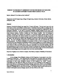
Fragility curves have been derived for four mechanical damage states, two of which are identified from the response of a single masonry pier, while the other two are found from the global pushover curve of the structure (Figure 1). The first damage state, DS1, corresponds to the attainment of the yield displacement δy of the bilinear approximation to the capacity curve of a single masonry pier. The bilinear approximation is obtained by fixing the initial stiffness as the secant to the point corresponding to 70% of the maximum resistance and the equivalent resistance so as to impose the coincidence of the area below the bilinear curve and the area below the capacity curve up to the ultimate limit state [3]. The δy obtained is always larger than the drift corresponding to 70% of the shear resistance and hence it is likely that some cracks have already occurred at such deformation value. The second damage state, DS2, is identified by the drift corresponding to the first shear cracking of the pier, δs. In this work, values of δs have been obtained from experimental results and in particular they were indicated in the experimental test report. Sometimes the first cracking is not easy to detect during experimental tests, especially if the wall surface is not painted or covered by plaster. For this reason experimental values associated with δs are typically larger than those of δy . The damage levels to DS3 and DS4 have been derived from global pushover curves of the building. In particular, DS3 corresponds to the the maximum shear resistance, while DS4 corresponds to 80% of that value.

90

60

30

8

0

Displacement [mm]

0

1

2

3

4

5

6

7

displacement [mm]

Figure 1. Left: identification of the damage states on a pushover curve; right: identification of the yield, cracking and ultimate drifts on the pushover curve of a single pier and its bilinear approximation.

258

Stochastic seismic assessment of unreinforced masonry buildings

3 STOCHASTIC MONTE CARLO SIMULATIONS To take into account the different sources of uncertainty involved in the seismic assessment of masonry buildings, a prototype building with a deterministic geometry and random material properties is defined. This randomness allows one to take into account both the fact that in most real cases, building properties are not well known and also the variability intrinsic in the definition of building typologies, grouping together buildings with different characteristics and mechanical properties. The uncertainty associated with modelling assumptions and incomplete knowledge of structural details has been neglected. A large number of Monte Carlo analyses are then performed, until convergence of both the input and output variables to their mean is reached and the value of standard deviation becomes stable. The uncertain parameters are sampled from their associated Gaussian probability distributions, which were previously defined based on experimental results. The sampled values are combined to define a series of structures with different characteristics, all nominally representing the same prototype building. Two sets of Monte Carlo analyses have been carried out. In the first type, values of the mechanical properties have been varied within the selected ranges and randomly assigned uniformly over the entire building model. In the second type, an additional randomness was introduced, with the creation of a library of randomly defined materials, which are then randomly assigned to the different structural elements of the model. This accounts for the fact that material properties of masonry buildings can vary significantly from element to element, even within the same structure. Monte Carlo stochastic simulations have been performed using a software called STAC, developed at the International Centre for Numerical Methods in Engineering (CIMNE) of Barcelona [4]. The software allows one to extract values from predefined probability distributions of the input variables of interest, then calls the structural program which runs the analysis and returns values of the output variables.

4 CASE STUDY BUILDING 4.1

Building description and model

The case study building is a 3-storey masonry building, typical of the construction typologies of the neighbourhood called Rione Libertà in Benevento (southern Italy), where it is located. It was constructed in 1952 and has plan dimensions of 17.7 x 14.3m and a height of 11.05m. The bearing walls are formed from masonry tuff units, with reinforced concrete floors and reinforced concrete tie beams guaranteeing the connection between floors and walls. Note that the geometry of the structure has been considered deterministic, whilst material characteristics are assumed as random variables, since this building is a prototype considered to be representative of a class of similar buildings. Figure 2 shows a picture and the typical plan of the building, together with a view of the 3D model obtained with the program TREMURI, which allows one to perform nonlinear seismic analyses of entire unreinforced masonry buildings. The capabilities of this software and the algorithms embedded in it are described in detail in several literature works (e.g. [5], [6], [7]). The program is based on the nonlinear macro-element model proposed by Gambarotta and Lagomarsino [8] and modified by Penna [5], representative of a whole masonry panel (pier or spandrel beam). 3D modelling of the building is based on the identification of the seismically resistant structure, constituted by walls and floors. The walls are the bearing elements, while the floors, apart from imparting vertical loads to the walls, are considered as planar stiffening elements (orthotropic 3-4 node membrane elements), on which the horizontal distribution of actions between the walls depends. The model is based on the hypothesis that the seismic response of the building is governed by a global box-type behaviour, assuming that local mechanisms (mainly out-of-plane) are prevented by appropriate structural details and/or connecting devices (e.g. tie rods or tie beams). With this assumption, the local flexural behaviour of the floors and the local out-of-plane wall response are not computed because they are considered negligible with respect to the global building response, governed by their in-plane behaviour. This is acceptable for this type of building, where stiff 259

Rota M., Penna A., Magenes G.

diaphragms and low height/thickness ratios for the walls render out-of-plane response a secondary phenomenon. Notice that a global seismic response is possible only if vertical and horizontal elements are properly connected. A frame-type representation of the in-plane behaviour of masonry walls is adopted, with each wall of the building subdivided into piers and lintels (2 node macro-elements) connected by rigid nodes. 0,6

0,3

0,75

17,7

Figure 2. Case study building located in Benevento: a picture (left), the plan of a storey (centre) and the building model (right).

4.2

Ranges of variation of the mechanical parameters

The mechanical parameters needed for the numerical model have been defined based on the experimental results of the tests carried out by Faella et al. [9] on tuff specimens. In particular, meaningful ranges of variation of the different parameters were defined by simulating, with the program TREMURI, the experimental results of the tests carried out on walls of type T1 and T2. Different cyclic pushover analyses were carried out, calibrating the model parameters until the fit with the experimental results was deemed to be satisfactory. Two examples of the comparison of experimental and numerical cyclic force-displacement curves are shown in Figure 3. 175 150

175

V [kN]

150

125

125

100

100

75

75

50

50

25

25

0

0

-25

-25

-50

-50

-75

-75

-100

-100

-125

-125

V [kN]

-150

-150

d [mm]

-175 -10

-9

-8

-7

-6

-5

-4

-3

-2

-1

0

1

2

3

4

5

6

7

8

9

d [mm]

-175 -10

10

-9

-8

-7

-6

-5

-4

-3

-2

-1

0

1

2

3

4

5

6

7

8

9

10

Figure 3. Comparison of experimental test results (grey thin curve) and numerical simulations (black thick curve) for two specimens: T1-1 (left) and T2-6 (right). Based on this comparison, only the parameters related to shear failure modes could be calibrated, since all tested specimens failed in shear: shear modulus G, initial shear resistance for zero compression (cohesion) fvo, friction coefficient µ, nonlinear shear deformability ratio Gc, softening parameter β, ultimate shear drift δv. The parameters that could not be obtained from experimental tests have been derived from the indications reported in Annex 11.D of the OPCM 3274 [3]. For what concerns the ultimate flexural drift δf, a mean value of 0.8% has been adopted, as also suggested in EC8-3 [10], with an assumed coefficient of variation of 10%. Table 1 summarises the range of values 260

Stochastic seismic assessment of unreinforced masonry buildings

and the parameters of the probability density function (pdf) for each mechanical quantity needed for the numerical analysis. Normal distributions have been assumed for all the mechanical parameters, with the mean value corresponding to the central value of the interval and the standard deviation such that the extreme values of the interval approximately correspond to the 95% percentile. Table 1 also shows the parameters of the pdf of the values of drift corresponding to first cracking. In particular, two sets of drift values are reported: δs corresponds to the first evidence of shear cracking and is obtained directly from the experimental tests; δy is the drift associated with the elastic limit of the equivalent bilinear approximation of the envelope capacity curve. The drift values directly obtained from the experimental tests can be found in [1]. Table 1.

Values of the parameters used in stochastic analyses E [MPa]

G [MPa]

fm [MPa]

fvo [MPa]

µ [-]

Gc [-]

β [-]

δv [%]

δf [%]

δs [‰]

δy [‰]

Min

1350

500

1.2

0.105

0.05

4

0.2

0.52

-

-

-

Max

1890

750

2.7

0.2

0.08

10

0.4

0.78

-

-

-

Mean

1620

625

1.95

0.1525

0.065

7

0.3

0.65

0.8

1.825

0.905

St. dev.

135

62.5

0.375

0.02375

0.0075

1.5

0.05

0.065

0.08

0.1125

0.128

Min

1350

500

1.2

0.105

0.05

4

0.2

0.52

-

-

-

5 NONLINEAR STATIC ANALYSES Nonlinear static (pushover) analyses have been carried out only in the x direction, since it appears the weak direction of the building and the first vibration mode is along the x direction. A force distribution proportional to the first vibration mode has been considered. In some cases, results of pushover analyses may be strongly affected by the choice of the control node; however, this is not an issue for this building, since rigid floors guarantee the same displacement at all nodes of the top storey. Two sets of 1000 stochastic pushover analyses have been carried out. In this paper only the second set will be discussed, in which the mechanical parameters are random variables and also the material associated with each macro-element is randomly selected from a predefined library of materials. In particular, each of the 30 different materials defined for the 165 structural elements is characterised by values of the mechanical parameters randomly selected from the intervals. Materials are then redefined for each analysis. The number of analyses performed was sufficient to observe convergence of each input and output variable to its mean value and stabilisation of the standard deviations. Some of the pushover curves obtained are shown in the left part of Figure 4 and the mean curve and the mean plus or minus one standard deviation are identified. Each pushover curve allows one to identify the two global limit states corresponding to the attainment of the maximum base shear resistance and to the ultimate condition, identified by a value of base shear equal to 80% of the maximum value. The mean value and the mean plus or minus one standard deviation values obtained form the 1000 analyses available are identified in the left part of Figure 4 by vertical lines. Notice that damage states were identified with reference to masonry piers. This is reasonable since the model accounts for coupling in the spandrel beams and the available experimental tests seem to allow one to exclude the necessity to impose specific drift limits for spandrel beams. The right part of Figure 4 shows the probabilistic relationship between global structural displacement and corresponding maximum element drift, which is necessary to derive the probability distribution associated with the damage state DS2.

261

Rota M., Penna A., Magenes G.

7

4000

6

Elements max drift [10-3]

Base Shear [kN]

3500 3000 2500 2000 1500 1000 500

5 4 3 2 1

0 0

0.5

1

1.5

2

2.5

3

3.5

4

4.5

5

5.5

6

6.5

7

7.5

0 0

Top Displacement [cm]

0.5

1

1.5

2

2.5

3

3.5

4

Global displacement [cm]

Figure 4. Left: Some of the obtained pushover curves, with identification of the mean and mean plus or minus one standard deviation curves. Vertical lines show global damage states. Right: relationship between global structural displacement and maximum element drift, with indication of the average and average plus or minus one standard deviation curves. Once the probability distribution of the maximum drift in the elements is known for each value of global displacement, the probability that this maximum drift exceeds the drift threshold associated to each damage state can be computed. Since the drift threshold of each damage level is also defined in terms of a probability distribution, the probability distribution relating DS1 and DS2 to the global structural displacement needs to be calculated by convolution of the two probability distributions. This procedure is shown qualitatively in Figure 5. For each global displacement value, the drift demand on the elements is evaluated and represented by a probability distribution of values (right part of Figure 5). The complementary cumulative distribution function (CDF) of such values (dashed line in the left part of the figure) is then convolved with the pdf of the two limit state thresholds (two bell curves in the left part of the figure). The result of the convolution for each DS is represented by the shaded areas in the figure. Such areas correspond to the integral of the joint probability distributions. Global displacement [cm] 2.5

2

2.25

1.5

1.75

1

1.25

0.5

0.75

0 0.0

0.5

1.0

1.5

2.0

2.5

3.0

3.5

0.25

pdf

0

0

0.25

0.25

0.5

0.5

1 1.25

δmax

1.25

1.5

1.5

1.75

1.75

Maximum element drift [%]

0.75

1

Maximum element drift [%]

0.75

2

2

2.25

2.25

2.5

2.5

Figure 5. Scheme of the procedure used for the identification of drift-dependent limit state probabilities.

262

Stochastic seismic assessment of unreinforced masonry buildings

6 INCREMENTAL DYNAMIC ANALYSES 6.1

Selection of accelerograms

Seven real accelerograms have been selected with the constraint of spectrum-compatibility with the target response spectrum of EC8, which corresponds to the one in the Italian seismic code [3], for a seismic zone 2, with an associated PGA of 0.25g. These records have been selected from strong motion record databases (www.isesd.cv.ic.ac.uk/, peer.berkeley.edu/smcat/, db.cosmos-eq.org/), through an algorithm that is described in detail in Dall’Ara et al. [2006], based on a Monte Carlo random selection of the groups of accelerograms better fitting the target spectrum. The selected accelerograms have been scaled linearly in order to match their PGA with the PGA of the target response spectrum. The scale factors applied to the accelerograms were all quite close unit, between 0.6 and 1.1. Notice that if a minimum of 7 accelerograms are applied to the structure, average results can be used instead of the most unfavourable ones, as suggested by several modern seismic codes ([3], [12], [13]) and research works [e.g. 14].

6.2

Results of incremental dynamic analyses

Incremental dynamic analyses have been carried out by applying to the structural model the accelerograms defined in the previous section, with a value of Rayleigh critical damping equal to 2%. A very large number of analyses would be required to take into account both the variability due to different ground motions (7 accelerograms) and the variability of mechanical parameters in the structural model. It is necessary to reduce the number of analyses, since each nonlinear time history analysis requires a significant computational time. A first set of time history analyses has been carried out using the mean value of each mechanical parameter and applying the 7 accelerograms scaled to a mean PGA of 0.05, 0.1, 0.15, 0.2, 0.25 and 0.3g. A second set of analyses has been carried out taking into account the variability due to material parameters and neglecting the variability induced by the different ground motion records. In this case, 100 realisations of each material parameter have been generated through Monte Carlo simulations and a corresponding number of analyses has been carried out, for a mean PGA of 0.1, 0.2 and 0.3g, by applying only the first accelerogram. For each considered PGA level, the total standard deviation associated to displacement demand has been calculated as the square root of the sum of the squares of the two standard deviations associated respectively to ground motion and mechanical parameter’s variability. To check the assumption that the variability related to ground motion has a stronger influence on displacement demand than the one due to mechanical parameters, the total standard deviation obtained with mean mechanical parameters and 7 accelerograms is compared in Figure 6 with that obtained with stochastic mechanical parameters and a single accelerogram. The figure shows that, for this prototype and with the selected accelerograms, the variability due to mechanical properties is significantly smaller then the variability induced by applying different ground motions. Hence, the assumption of neglecting the variability associated to different values of material parameters and work with the mean values seems acceptable. However, further analyses for different building prototypes and ground motion records are needed to confirm this finding. The probability density functions of maximum displacement demand at different values of PGA have been obtained from time history analyses with the 7 accelerograms scaled to each PGA value. The parameters of the corresponding lognormal distributions of the displacement demand have been derived from the hysteretic cycles obtained from these time history analyses, by identifying the mean and the standard deviation of the maximum displacement demand. As an example, the right part of Figure 6 shows the hysteretic cycles obtained from all the time history analyses with the 7 accelerograms scaled to a PGA of 0.1g: the mean and mean plus or minus one standard deviation value of the Figure 7 maximum displacement demand obtained from the different analyses are indicated by vertical lines. shows the complementary cumulative distributions of displacement demand, which will be convolved with the distributions of each damage state, in order to derive fragility curves. 263

Rota M., Penna A., Magenes G.

4000 3000

Base shear [kN]

PGA [g]

0.3

0.2 Total st.dev. Mean parameters, 7 acc. st.dev. Stochastic parameters, 1 acc. st.dev.

0.1 0

0.5

1

1.5

2

2.5

3

2000 1000 0 -1.5

-1

-0.5

-1000

0

0.5

1

1.5

-2000 -3000

Standard deviation of max. displacement [cm]

-4000

Top displacement [cm]

Figure 6. Left: comparison of standard deviations obtained with mean mechanical parameters and 7 accelerograms, with stochastic parameters and only 1 accelerogram and combining the two cases. Right: identification of maximum displacement demand (mean and mean plus or minus one standard deviation) for a PGA of 0.1g. 1.0

0.3g

1 - CDF

0.8 0.6

0.25g

0.15g

0.4 0.2

0.05g

0.2g

0.1g

0.0 0

1

2

3

4

5

6

7

8

Displacement [cm]

Figure 7. Complementary cdfs of the displacement demand at different PGA levels.

7 SEISMIC RELIABILITY ASSESSMENT Fragility curves have been obtained with the procedure shown in Figure 8.

1-Cdf(0.25g) Pdf(DS1) Pdf(DS2) Pdf(DS3) Pdf(DS4) Pf(DS1) Pf(DS2) Pf(DS3) Pf(DS4)

Probability [-]

2.5

2.0

1.5

1.0

0.5

0.0 0

1

2

3

4

5

6

7

8

Displacement [cm]

Probability of exceeding damage states

PGA = 0.25 g

3.0

1 DS1

0.9 0.8

DS2 DS3

0.7

DS4

0.6 0.5 0.4 0.3 0.2 0.1 0

0

0.05

0.1

0.15

0.2

0.25

0.3

PGA [g]

Figure 8. Derivation of the fragility points for a PGA = 0.25g, from convolution of pdf of the different limit states and complementary CDF of demand..

264

Stochastic seismic assessment of unreinforced masonry buildings

Probability of exceeding damage states

The top part of figure 8 shows the complementary cumulative distribution function of the displacement demand obtained from time history analyses (dashed-dotted line) and the probability density functions of the various damage states obtained from pushover analyses (continuous bell curves), for a PGA of 0.25g. These curves are convolved and the obtained curves are shown, for each damage state, with a dashed bell curve under the corresponding continuous bell curve. The integral of the area below the curve representing the result of the convolution gives a value of probability, i.e. the probability of exceedence of that damage state for a PGA of 0.25g. These values are then reported as points in the right part of figures and represent the fragility points corresponding to this PGA level. This procedure has been repeated for all the considered PGA values, and the various fragility points obtained have been fitted using a lognormal probability distribution function. The lognormal curves fitting them are plotted in the left part of Figure 9, while the parameters (µ and σ) of the lognormal curves are summarised in Table 2. 1

Table 2.

DS1

0.9

DS2

0.8

DS3

0.7

DS4

0.6 0.5 0.4 0.3 0.2 0.1 0

0

0.05

0.1

0.15

0.2

0.25

Parameters of the lognormal distributions

DS

µ

σ

DS1

-2.026

0.362

DS2

-1.645

0.273

DS3

-1.351

0.218

DS4

-1.169

0.175

0.3

PGA [g]

Figure 9. Lognormal fragility curves fitting the analytically derived fragility corresponding parameters of the lognormal curves are reported in Table 2.

points.

The

8 CONCLUSIONS The paper presents an innovative methodology for the assessment of seismic reliability of single masonry buildings, based on detailed 3D nonlinear dynamic analyses of the entire structure. In order to illustrate the procedure, application to a case study building is presented. It is modelled with deterministic geometry but considering all mechanical properties of the structure as random variables, with normal probability distributions defined based on experimental results and other sources of information. Monte Carlo simulation is used to extract values of each parameter from the corresponding probability distribution and randomly assign them to each structural element. Nonlinear static analyses are carried out to define the probability density functions of selected damage thresholds, which are then convolved with the probability distribution of maximum displacement demand obtained from nonlinear incremental dynamic analyses. Lognormal fragility curves representative of the seismic reliability of the building are hence obtained, by fitting the fragility points, i.e. the probability of exceeding different damage levels for discrete PGA levels. Although the proposed approach still needs to be further tested and improved by applying it to different building prototypes, it represents a step forward in the definition of analytical models for the seismic reliability assessment of masonry buildings. Being based on advanced nonlinear analyses of entire buildings, it is also rather different from the other approaches available in the literature, which are often based on very simplified models of the buildings and/or approximate analysis types (linear or nonlinear static analyses).

265

Rota M., Penna A., Magenes G.

ACKNOWLEDGEMENTS The authors would like to thank Prof. Alex Barbat of the Universitat Politècnica de Catalunya, Barcelona, for kindly providing the program STAC used to perform Monte Carlo simulations. The financial support of the Reluis Project (Line 10) "Definition and development of databases for risk evaluation and emergency management and planning” is also acknowledged.

REFERENCES [1]

[2] [3]

[4]

[5] [6]

[7] [8]

[9]

[10] [11]

[12] [13] [14]

Rota, M., Penna, A. & Magenes, G. A methodology for deriving analytical fragility curves for masonry buildings based on stochastic nonlinear analyses. Engineering Structures (2010), doi:10.1016/j.engstruct.2010.01.009 Galasco, A., Lagomarsino, S. & Penna, A. TREMURI Program: Seismic Analyses of 3D Masonry Buildings, University of Genoa, Italy, 2006. OPCM 3274. Ordinanza del Presidente del Consiglio dei Ministri n. 3274 del 20 Marzo 2003: Primi elementi in materia di criteri generali per la classificazione sismica del territorio nazionale e di normative tecniche per le costruzioni in zona sismica. GU n. 72 del 8-5-2003, with further modifications in OPCM 3431, 2005 – in Italian. Zárate, F., Hurtado, J., Oñate E. & Rodríguez, J. STAC program: stochastic analysis computational tool, CIMNE, Centro Internacional de Métodos Numéricos en la Ingeniería, Barcelona, España, 2002. Penna, A. A macro-element procedure for the non-linear dynamic analysis of masonry buildings. Ph.D. Thesis, Politecnico of Milan, Italy – in Italian. Lagomarsino, S. & Penna, A. A nonlinear model for pushover and dynamic analysis of masonry buildings, In: Proc. Int. Conf. on Computational and Experimental Engineering and Sciences, Corfu, Greece, 2003. Galasco, A., Lagomarsino, S., Penna, A. & Resemini, S. Nonlinear seismic analysis of masonry structures, In: Proc. 13th WCEE, Vancouver, Canada, 2004, Paper No. 843. Gambarotta, L. & Lagomarsino, S. On dynamic response of masonry panels. In: Proc. Nat. Conf. “La meccanica delle murature tra teoria e progetto”, ed. L. Gambarotta, Messina, Italy, 1996 - in Italian. Faella, G., Manfredi, G. & Realfonzo, R. Comportamento sperimentale di pannelli in muratura di tufo sottoposti ad azioni orizzontali di tipo ciclico. In: Proc. 5th It. Conf. Earthquake Engineering, Palermo, 1991 – in Italian. EC8-3 ENV 1998-3 Eurocode 8: Design of structures for earthquake resistance - Part 3: Assessment and retrofitting of buildings, 2005. Dall’Ara, A., Lai, C.G. & Strobbia, C. Selection of spectrum-compatible real accelerograms for seismic response analyses of soil deposits. In: Proc. 1st ECEES, Geneva, Switzerland, 2006, Paper No. 1240. UBC Uniform Building Code. Structural engineering design provisions, Vol. 2, International Conference of Building Officials, California, U.S.A, 1997. EC8-1 ENV 1998-1 Eurocode 8: Design of structures for earthquake resistance – Part 1: General rules, seismic actions and rules for buildings, 2005. Bommer, J.J., Acevedo, A.B. & Douglas, J. The selection and scaling of real earthquake accelerograms for use in seismic design and assessment. In: Proc. ACI Int. Conf. Seismic Bridge Design and Retrofit, California, 2003.

266