Stock price direction prediction by directly using prices data - arXiv
Recommend Documents
A novel approach to predict future market direction has been introduced based on chart patterns .... analysis mainly focuses on the chart and quantitative data.
Stock Price Prediction Using the ARIMA Model. 1Ayodele A. Adebiyi., 2Aderemi
O. Adewumi. 1,2School of Mathematic, Statistics & Computer Science. University
...
The prediction was done by a nonlinear fuzzy-neural network model using exogenous variable of stock market. General Terms. Artificial Intelligence, Artificial ...
Apr 25, 2017 - Data Mining algorithms together with Text Mining techniques and. Linguistics started to be applied in financial market. Supported by Behavioral ...
The prediction was done by a nonlinear fuzzy-neural network model using exogenous variable of stock market. General Terms. Artificial Intelligence, Artificial ...
domain knowledge which was encoded in them using Rough Sets. The pool of ... despite a downtrend in stock prices and low turnover in stock exchanges.
Apr 29, 2016 - conditions, investors' sentiments towards a particular company, political ..... we trained a random forest using the Apple Dataset for a time ...
technical analysis and using advanced math and science. Extensive attention has been dedicated to the field of artificial intelligence and data mining techniques ...
Investments in stock markets involve very high risk due to its complexity and ... Analysis, 2) Time Series Forecasting, 3) Machine Learning and 4) Modeling and ...
Apr 29, 2016 - current stock prices fully reflect all the relevant information. It implies that if someone ...... 0.96120. 0.92341. Fig 7: Results for Apple Inc. dataset.
Apr 29, 2016 - Luckyson Khaidem, Snehanshu Saha and Sudeepa Roy Dey. (Received 00 Month 20XX; accepted 00 Month 20XX). Abstract Predicting trends ...
Comparison between support vector machine and fuzzy Kernel C-Means as ... In this study, two models of machine learning applied to predict stock price.
DIRECTION BASED ON NEWS ARTICLES. Hakan Gunduz ... this study, we got news articles from three big financial .... they used the Support Vector Machines.
May 17, 2015 - Predicting stock price movement is generally accepted to be challenging such that until today it is continuously ... Instead of making a comparison between classification models, .... Suppose for the unit cube integration domain. [ ].
researchers over the years to develop better predictive models. The autoregressive ... Keywords- ARIMA model, Stock Price prediction, Stock market, Short-term ...
The advances of data mining and text mining techniques for this ... in terms of investment recommendation for financial market, and the successful use of.
alignment between news articles and stock prices, pre-processing, and classifier ...... found out the interaction effect between Twitter and news sentiment has a ...
The focus of this paper is to present a generic stock price prediction model ..... W. Ziarko, R. Golan and D. Edwards (1993) An application of datalogic/R ... International Workshop on Intelligent Systems Design and Applications, Com- putational ...
Mar 6, 1998 - movements in the stock market for the 30 companies listed in the Down Jones Industrial. Index (DJIA) ...... Travelers Companies Inc. 1,001.
Mar 1, 2018 - Considering the importance of stock price prediction, this study tends to predict ... 2.2 Genetic Algorithms: Genetic algorithm [8] is a biological ...
analysis based on a modified kNN to determine where correlated areas fall in the .... advanced predicting models to help the financial markets and brokerage ...
May 17, 2015 - Potchefstroom, Republic of South Africa ... Sciences, Muizenberg, Cape Town, Republic of South Africa ...... Anglo American Platinum Plc.
Index TermsâTime series, Stock market, RNN,LSTM,CNN. I. INTRODUCTION. Forecasting can be defined as the prediction of some future event or events by ...
of both linear (AR,MA,ARIMA) and non-linear algorithms. (ARCH,GARCH ... Index TermsâTime series, Stock market, RNN,LSTM,CNN. I. INTRODUCTION.
Stock price direction prediction by directly using prices data - arXiv
the KOSPI and HSI', Int. J. Business Intelligence and Data Mining, Vol. ... of a stock market and yet reported that the best prediction performance that he could ..... and Osburn, L. (1993) 'Forecasting S&P and gold futures prices: an application of.
Market Index and Stock Price Direction Prediction using Machine Learning Techniques: An empirical study on the KOSPI and HSI Yanshan Wang∗ School of Industrial Management Engineering, Korea University
Abstract The prediction of a stock market direction may serve as an early recommendation system for short-term investors and as an early financial distress warning system for long-term shareholders. In this paper, we propose an empirical study on the Korean and Hong Kong stock market with an integrated machine learning framework that employs Principal Component Analysis (PCA) and Support Vector Machine (SVM). We try to predict the upward or downward direction of stock market index and stock price. In the proposed framework, PCA, as a feature selection method, identifies principal components in the stock market movement and SVM, as a classifier for future stock market movement, processes them along with other economic factors in training and forecasting. We present the results of an extensive empirical study of the proposed method on the Korean composite stock price index (KOSPI) and Hangseng index (HSI), as well as the individual constituents included in the indices. In our experiment, ten years data (from January 1st, 2002 to January 1st, 2012) are collected and schemed by rolling windows to predict one-day-ahead directions. The experimental results show notably high hit ratios in predicting the movements of the individual constituents in the KOSPI and HSI. The results also imply the co-movement effect between the Korean (Hong Kong) stock market and the American stock market. c 2013
Keywords: stock direction prediction, principal component analysis (PCA), support vector machine (SVM), KOSPI, HSI
1. Introduction Nowadays investors have been more keenly aware of risk than any time in the past due to the non-stationary and chaotic stock markets under the impact of the US subprime crisis. Simultaneously, they hope to gain a great profit from the investments. But, it is extraordinarily difficult to perform better than skilled and knowledgeable competitors in a stock market. Better stock prices direction prediction is a key reference for better trading strategy and decision making by ordinary investors and financial experts [1]. Apart from the stock price direction prediction, the stock market index direction prediction is regarded as one of the crucial issues in recent financial analysis studies. The stock market index measures overall market behavior through selected stocks representing the market. Accurate index direction prediction provides investors with information regarding the expectations about the movement behavior of the economy and return obtained by a specific investing portfolio [2]. Also it is an early warning system for investors, notably for short-term investors, against sudden drops in the market.
The emergence of machine learning and artificial intelligence algorithms has made it possible to tackle computationally demanding mathematical models in stock price direction prediction. Frequently adopted methods include Artificial Neural Networks (ANNs), Bayesian Networks, and Support Vector Machine (SVM). Amongst them, ANNs have drawn significant interests from several researchers in the stock price forecasting in the past decades. The ANNs are robust in model specification compared to parametric models, which makes it frequently applied in forecasting stock prices and financial derivatives. Guresen, et al. [3] reported the validity of ANNs in stock market index prediction. Cheng, et al. [4] forecasted US treasury bond with a ANNs-based system. Grudnitski & Osburn [5] applied ANNs to predict gold futures prices.The drawback of the price prediction is that the price is highly volatile so as to result in large regression errors. Compared to the price prediction, the stock direction prediction is less complex and more accurate [6]. The stock direction prediction has been recently addressed in several research articles, which consider different variants of ANNs [7]. However, one drawback of ANNs is that the efficiency of predicting unexplored samples decreases rapidly when the neural network model is too over-fitted by available observations. In other words, the noisy stock information may lead ANNs to a complex model, which might result in the over-fitting problem. The predominant methods in the stock market direction prediction are the approaches based on Support Vector Machine (SVM) [8–10]. Since the SVM implements the structural risk minimization principle, it often achieves better generalization performance and lower risk of overfitting than the ANNs [11]. This point in regard to stock prediction is well braced by Kim [9]. His experiment showed that the SVM outperformed the ANNs in predicting future direction of a stock market and yet reported that the best prediction performance that he could obtain with SVM was 57.8% in the experiment with the Korean composite stock price index 200 (KOSPI 200). Huang et al [8] reported remarkable performance of 75% hit ratio by using a SVM-based model to predict Nihon Keizai Shimbun Index 225 (NIKKEI 225) in a single period. However, the shortcoming in the most of literature is that the testing used was conducted within the in-sample datasets, or that the out-of-sample testing was on small data sets which were unlikely to represent the full range of market behaviors. Thus it is difficult to assess the average performances of their models in multiple periods such as Kim nor Huang et al conducted the experiment in that setting. In order to refrain from limited sample selection, our experiments computed the one-day-ahead predictions using rolling windows of data to ensure that the predictions are made using all the information available at that time, while not incorporating old data that are probably no longer relevant in the context of a dynamic, rapidly evolving stock market. A major drawback of SVM for the direction prediction is that the input variables lie in a high-dimensional feature space, ranging from hundreds to thousands. The storage of the variables requires a lot of memory and computation time. Specifically, a stock market consists of several hundreds of stocks, which leads to the high dimensionality of the variables. Therefore, it is of considerable importance to conduct dimension reduction to acquire an efficient and discriminative representation before classification. Under the dimensionality reduction, curse of dimensionality could be effectively managed [11]. A common unsupervised feature extraction method is Principal Component Analysis (PCA) [12] by which principal components are obtained through the manipulation of original data. The PCA has been widely used to deal with high dimensional data sets in many areas, such as protein dynamics reduction, spectral data reduction, and face patterns reduction. Interestingly, the adaptation of the PCA feature selection to stock prices data analysis is rarely found, to the best of our knowledge. In stock prices data, there exits a common phenomenon that is called co-movement between stocks due to the institutional investors common ownership of subsets of stocks in their portfolios [13]. The co-movement implies that the utilization of PCA is essential for finding principal components among high correlated stock prices data. So the PCA is considerable for pre-using as a feature selection method for the SVM to obtain principal components amongst internal factors in the stock market. As a matter of fact, the co-movement exits not only between stocks in a domestic market but also between two tightly connected stock markets. For example, Shiller showed the co-movements of returns between the U.S. and U.K. markets [14]. The same phenomenon also exists between the U.S. stock market the Asian markets, as reported by Liu et al. [15]. These facts stimulate us to consider both internal and external factors for predicting individual stocks and market index directions. The macroeconomic indicators (such as CPI (consumer price index), GNP (gross national product) and GDP (gross domestic product)) may be high impact factors in the prediction. However, daily data of those macroeconomic factors are impossible to obtain and analyze in reality. For simplicity and generality, we only handle stock prices data which are timely and easy to access. Thus the process in this article is more practical than 2
3
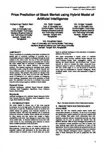
most of the state-of-the-art approaches. This paper is organized as follows. In the next section, we provide a brief overview of PCA and SVM and describe how they are integrated in our model. In Section 3, we present detail descriptions on the empirical experiment, which includes the detailed design of experimental data and experiment results. The last section concludes this paper with some discussions. 2. An Integrated Model The structure of the proposed model is shown below in Fig. 1. Let xi ∈ R p denote a column vector of the daily rates of return of stock i, i = 1, ..., n, which is obtained from p daily market observations. The matrix X = (xi )T can be reduced to the principal component matrix Y = (yk )T , k = 1, ..., m, m n by minimizing the variance of the linear transformation of X. Define the contribution rate of the kth principal component as Pnλk λi where λk represents the variance of yk . The cumulative rate of the first m principal components is
Pm λ Pni=1 i . i=1 λi
i=1
Along with these principal components, internal factors and external factors F = (F1 , F2 , ..., Fh )T are utilized as input data, i.e. {Y, F}. Considering the co-movement property in a market, we find that the co-moved stocks are informative as internal factors. Besides, since the market index itself is a beacon of the domestic economy and tread, it is also informative for forecasting. In addition to the internal factors, external factors also play important role in the Asia stock markets. Here we consider two foremost economic phenomenons. The U.S. is the largest cooperative partner for Asian countries, including Korea and Hong Kong, thus the conditions of the U.S. financial market have significant impacts on Asian stock market. The other is the exchange rates (EXR) that also has strong influence on the imports and exports of products. The changes of trading relations in turn affect the domestic stock markets. Thus, the external factors used in our study include the S&P 500 Index in the U.S. stock market, the best representation of the U.S. economy, and the exchange rate, the symbol of trades between countries. Details of the data are explained in Section 3. The input to SVM is the data set R = (r j , w j ), where r j = (Y j , F j )( j = 1, ..., p) is a row vector denoting jth daily data in p observation days. w j ∈ 0, 1 is a binary variable that represents the upward or downward direction of the stock market movement of the jth day. The downward direction is represented by 0 and the upward by 1. The input data is carefully divided into two parts, i.e. training data and testing data. As addressed by financial analysis recently, the data periods in most computer technique related articles are selected limitedly. In order to refrain from limited sample selection, the training data and testing data are goes parallel using rolling windows of ten years data to ensure that the predictions are made using all the information available at that time. Besides, unlike several studies testing in-sample data, we compute the one-day-ahead predictions, i.e. out-sample data. The details of data periods and how they are divided into training and testing data are explained in the next section. The training data is utilized to acquire a classifier by training SVM. The classifier function of stock movement directions is defined as p X ∗ ∗ T dir = f (r) = sgn w j α j r j r + ν , (1) j=1
where α s and ν s are optimal values of Lagrange multipliers and intercepts of the corresponding hyperplanes, respectively. By introducing kernel tricks, the nonlinear decision function for a stock direction prediction becomes p X dir = f (r) = sgn w j α∗j K(r j , r) + ν∗ . (2) ∗
∗
j=1
The selection of kernel function is addressed in Section 3. The testing data is used to test the model according to the classifier f (r). In reality, the training model can be designed to update real-timely so as to make full use of the present information. 3
4
Stocks Data:
X Factors Data:
F
PCA
{
Data Pool for SVM: Y j , F j
Training part
}.
Testing part
Training Data
Testing Data
SVM
SVM Classifier
Results
Figure 1. Procedure of the proposed PCA-SVM integrated model.
4
5
3. Empirical Experiment In this section, we present the empirical stock price data sets, time periods and data designs for the proposed method. In order to avoid the fact that some markets are less efficient than others, we test empirical experiments on two representative Asia stock markets: the Korean stock market and the Hong Kong stock market. The experiments aim to forecast the directions of daily movements of the stock price indices and of individual stocks. 3.1. Experiment Data 3.1.1. Stock Market Indices The Korea composite stock prices index 200 (KOSPI 200) and the Hang Seng index (HSI) are utilized since they represent the overall performance of the Korean and the Hong Kong stock market. As an underlying index for stock index futures and options, KOSPI 200 consists of the two-hundred companies chosen from all stocks in the KRXStock Market. The KOSPI 200 represents a broad cross-section of Korean industries and provides an effective means for investors to avoid potential market risks. Thus, the 200 individual stocks daily rates of return are utilized. Similarly the HSI is the main indicator of the overall market performance in Hong Kong and the 48 constituents are processed in our empirical approach. We note that all the data are collected from publicly available sources in the internet. The KOSPI 200 data set are collected from KRX Korea Exchange 1 . HIS data set are collected from YAHOO! Finance 2 . 3.1.2. Factors As addressed in the preceding and the structure of the method (Fig. 1), internal factors co-movement stocks considered amongst the stock market and the market index. For forecasting indices, we use the lagged daily prices for indices and the overall constituents. As for individual stock prediction, we use the lagged daily prices for the target-excluded constituents besides indices. The external factors used in our study include the S&P 500 Index in the US stock market and the exchange rate of US dollars to Korean Won (USDKRW) or Hong Kong Dollar (USDHKD). The S&P 500 Index data and USDKRW (USDHKD) data are downloaded from YAHOO! Finance 2 and International Monetary Fund 3 , respectively. Because the opening days of the markets in Asia markets and US are different, the data are aligned based on the Asia markets timeline. The dealing strategy is that redundant daily data are deleted while missing daily data are filled by the previous closing price. 3.1.3. Time Periods In order to avoid limited sample selection, the data sets tested in our empirical experiment are gathered for the time periods of 2002 to 2011. Unlike most of the studies that tested machine learning methods within in-sample data, we tested the proposed method using out-sample data. Besides, a rolling window design of data was used so as to fully check the performance of the method and ensure that the predictions were made using all the information available at that time. The time periods of the rolling window data are shown in Table 1. In short, we treat three years training data and the following years testing data as a window which slides from the first year until the end of the ten years period. 3.1.4. Data Pre-process Instead of using the daily rate of return directly, we transform it into an n-day relative difference in percentage of price (RDP). The advantage of the transformation is that the distribution of the transformed data will be more symmetrical and close to a normal distribution [10]. In this paper, the RDP values are determined based on three-day-lagged values (RDP-3) for the indices and EXR, and one-day-lagged (RDP-1) for the constituents of KOSPI and HSI. The reason of choosing three-day-lagged values for the formers is that market indices and EXR changes always have delayed-effects on the index values [14]. Since the constituents serve as market comprising elements, the co-movements between the elements affect the market itself immediately. Therefore, a shorter lagged period is selected. The direction to forecast is the sign of one-day-ahead RDP, which is denoted as RDP+1. The detailed calculations for all the indicators are given in Table 2. 1 available
at: http://eng.krx.co.kr at: http://finance.yahoo.com 3 available at: http://www.imf.org 2 available
5
6
Table 1. Corresponding time period of training and testing data.
Iteration 1 2 3 4 5 6 7
Training Period 2002-1-1 2005-1-1 2003-1-1 2006-1-1 2004-1-1 2007-1-1 2005-1-1 2008-1-1 2006-1-1 2009-1-1 2007-1-1 2010-1-1 2008-1-1 2011-1-1
3.2. Direction Forecasting for indices and individual stocks Our task is to forecast the daily direction of KOSPI (or HSI) and the movement directions of the constituent stocks in KOSPI (or HSI). From equation (2), the direction function can be written as follows RDP−3 RDP−3 RDP−3 dirRDP+1 = f (FIndex , FS&P500 , FEXR , Y1RDP−1 , Y2RDP−1 , ..., YkRDP−1 ),
(3)
RDP−3 RDP−3 RDP−3 are the RDF-3 values of the KOSPI (or HSI), the S&P 500 Index and the exchange where FIndex , FS&P500 , FEXR rates of USD against KRW (or HKD), respectively. Y1RDP−1 , Y2RDP−1 , ..., YkRDP−1 are principal components of all the constituents with the input defined by RDF-1 value of the stocks in KOSPI (HSI). dirRDP+1 is a categorical variable that is obtained from the SVM classifier and represents the movement directions of the prices, i.e. 1, price increases, RDP+1 dir = (4) 0, price decreases,
Note that the direction is assigned to 1 if the closing value is the same as the previous closing value. 3.3. Experiment Results 3.3.1. Results of the PCA Fig. 2 and Fig. 3 depict the contribution rate (histogram) and cumulative distribution (line) of the first several components of the constituents in KOSPI and HSI over the whole time period respectively. The cumulative contribution is plotted by accumulating the contribution rate. From the following figures we find that the first component has over 70% contribution for the KOSPI and the first 10 components have over 70% for the HSI. Thus the first 1 while the first 10 components are chosen as principal components for the KOSPI and HIS to predict the dirRDP+1 , respectively . 3.3.2. Interpretations and Hints of the PCA In this subsection, a 2-dimensional illustrative example of the PCA is given for visualizing the principal components, as shown in Fig. 4. The first two stocks in KOSPI, SamsungElec and HyundaiMtr, are selected under observations over the whole periods. All the data are scaled to have a mean of zero. So the principal components can be represented by two orthogonal arrows passing through the origin with greatest variance. The thick line represents the first principal component and the dashed line represents the second principal component. Both arrows are the vectors that are derived from the eigenvectors of the covariance matrix that are scaled by the corresponding eigenvalue. 6
Rate
7
90
90%
80
80%
70
70%
60
60%
50
50%
40
40%
30
30%
20
contribution rate cumulative rate
10 0
1
2
3
4
5 6 7 Principal Component
20% 10% 0%
8
Rate
Figure 2. Contribution rates of principle components for the KOSPI.
90
90%
80
80%
70
70%
60
60%
50
50%
40
40%
30
30%
20
contribution rate cumulative rate
10 0
1
2
3
4
5 6 7 Principal Component
8
9
Figure 3. Contribution rates of principle components for the HSI.
7
10
20% 10% 0%
8
0.15
0.1
HyundaiMtr
0.05
0
−0.05
−0.1 PC 1 PC 2
−0.15
−0.15
−0.1
−0.05 0 SamsungElec
0.05
0.1
0.15
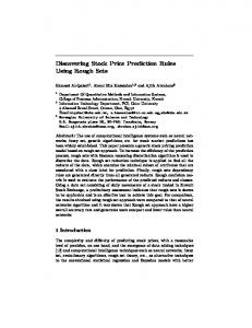
Figure 4. The plots of the first two principal components in KOSPI: Samsung Elec. and Hyundai Mtr..
Then the space is rotated so that principal components are aligned with the coordinate axes. In doing so, the data are uncorrelated in the principal component space. A biplot is helpful in digging some hints of the PCA. The biplot plots the projection of the loadings of the stocks on to the first two principal components. The biplot figure for the KOSPI and HIS are shown in Fig. 5 and Fig. 6, respectively. The plots reflect the phenomenon of co-movements, because the co-moved constituent stocks are near to each other and construct to a cluster. Empirically, we observe that those highly correlated stocks in one cluster are from the companies in a similar domain area (e.g. SKTelecom, KT and KT&G) or that some of the correlated companies are sub-companies and sub-branches of the other companies (e.g. Samsung braches and Samsung Co., LG branches and LG Co.). 3.3.3. Results of the direction forecasting on the KOSPI and HSI There are two decisions to make for SVM classifier. One is the choice of a kernel function to use, i.e. linear, polynomial or radial basis function (RBF). The other is the selection of parameter C. Several studies have suggested the RBF kernel function [8–10] which is also used in our experiment. As for the parameter C, a small value causes under-fitting of the training data and a large value causes over-fitting. Therefore, a value between 0.1 and 1000 is known to be the appropriate choice for the parameter C. In our experiment, C = 100 is used since it is tested in the previous studies [9, 10]. Given the RBF kernel and C = 100 for the SVM classifier, we examine the effectiveness of the proposed method in forecasting indices. Comparisons of the accuracies are shown in Table 3 and Table 4 for the KOSPI and HIS respectively. To compare with the performance of the SVM, we also test the ANN and Random Walk (RW) as the benchmark. Besides, we input identical principal components for both the SVM and ANN to verify the influence of the PCA. From the tables, the RW model performs moderately. The influence of the PCA is obvious positive since both the 8
9
0 0
1
2
3
4
5
−3
x 10
0.005
KT&G
KT
SKTelecom
0.01
Samsung;SDI;Co.
SamsungElec
LGCHEM
LG;Corp.
HHI
KorZinc
0.015 Component 1
SamsungHvyInd
0.02
HyundaiSteel
HyundaiMtr
HyundaiMercMar
SamsungC&T Mobis
HyundaiEng&Const
Samsung F&Mlns DHICO
POSCO
S−Oil
KiaMtr
SamsungElecMech
DSME
OCI
0.025
SamsungSecu
0.03
SamsungEng
GS;E&C
Figure 5. Biplot of the KOSPI. The horizontal and vertical axes represent the first and the second principal components, respectively. The co-moved stocks are circled by the red ellipses.
Component 2
6
9
10
−0.3 0
−0.2
−0.1
0
0.1
0.2
0.3
0.4
CNOOC CHINA MRCH.HDG.INTL. COSCO PACIFIC CHINA RES.ENTERPRISE HONG KONG EXS.& CLEAR.
CITIC PACIFIC
CHINA PTL.& CHM PETROCHINA
0.05
0.1
0.15 0.2 Component 1
0.25
CHINA MOBILE HSBC HDG. (ORD $0.50) CHINA UNICOM CLP HOLDINGS POWER ASSETS HOLDINGS BANK OF EAST ASIA HANG SENG BANK HONG KONG AND CHINA GAS CATHAY PACIFIC AIRWAYS MTR HUTCHISON WHAMPOA HANG LUNG PROPERTIES CHEUNG KONG HOLDINGS SWIRE PACIFIC WHARF HOLDINGS SUN HUNG KAI PROPERTIES ESPRIT HOLDINGS HENDERSON LD.DEV. LI & FUNG NEW WORLD DEV SINO LAND
TINGYI CYMN.ISLE.HLDG. HENGAN INTL.GP.
KUNLUN ENERGY
CHINA OS.LD.& INV
0.3
ALUMINUM CORP.OF CHINA
CHINA RESOURCES LAND
0.35
Figure 6. Biplot of the HSI. The horizontal and vertical axes represent the first and the second principal components, respectively. The co-moved stocks are circled by the red ellipses.
PCA-SVM and PCA-ANN outperforms the original SVM and ANN respectively. The average hit ratios of the proposed PCA-SVM on forecasting the KOSPI and HIS are minorly better than the PCA-ANN. However the derivations of the ANN based methods are bigger than the SVM. This fact reflects the drawbacks of the ANN that refer to the volatility and over-fitting problems, which is clearer from the tables. On the other hand, we analyze the iteration 4, the period of 2008, when the subprime crisis occurred. The PAC-SVM performs moderately during that period but still better than the RW model. However, the ANN is untrustworthy because of the enormous difference between two indices forecasting results.
3.3.4. Results of the direction forecasting on the constituents The second experiment of forecasting directions of the constituents of the KOSPI and HSI is carried out with the proposed PCA-SVM, ANN and RW. In this paper, we report four sample constituents from the KOSPI (SamsungElec (SAEL), HyundaiMtr (HYMT)) and the HIS (BANK OF EAST ASIA (BOEA), CITIC PACIFIC (CIPA)), as shown in Table 5, 6, 7, and 8. Unlike the market indices direction prediction, the hit ratios of forecasting individual constituents are averagely better. The influence of the PCA is also noticeable as well as that of the previous section. The PCA-SVM gives higher average hit ratios with lower standard derivation compared with the PCA-ANN. All the testing experiments show that the methods using the PCA perform better. To summarize, the proposed method are considerably trustworthy in forecasting movement directions. 4. Conclusions and Future Research In this paper, we have proposed a PCA-SVM integrated model to forecast the directions of the stock market indices and the individual stock prices. In the model, the principal components identified by the PCA are used along with internal and external financial factors in SVM for forecasting. We have also presented an extensive empirical experiment based on the KOSPI and HSI. The results of the empirical experiments show that the proposed method provides markedly high hit ratios for forecasting movement directions of the constituents in the KOSPI and HSI. Since 11
our experiments computed the one-day-ahead predictions using rolling windows data of a long period, the results are not the product of limited sample selection but reliable with all the available information at that time. Our results also verifies the co-movement effect between the Korean (or Hong Kong) stock market and the American stock market because of the usage of S&P 500 and exchange rates. As a future study, a theoretical study on the performance of the proposed method is of worth. The clustering of the co-moved stocks according to the biplot needs a further investigation. The theoretical analysis of the better performance on forecasting the constituents is also worth studying. Moreover, other feature selection methods, for example, deep belief networks (DBN), may be also efficient to extract the features of the stock prices for classifiers, which is subject to another future research. References [1] L.-J. Kao, C.-C. Chiu, C.-J. Lu, J.-L. Yang, Integration of nonlinear independent component analysis and support vector regression for stock price forecasting, Neurocomputing. [2] B. V. Pathak, et al., The Indian Financial System: Markets, Institutions and Services, Pearson Education India, 2011. [3] E. Guresen, G. Kayakutlu, T. U. Daim, Using artificial neural network models in stock market index prediction, Expert Systems with Applications 38 (8) (2011) 10389–10397. [4] W. Cheng, W. Wagner, C.-H. Lin, Forecasting the 30-year us treasury bond with a system of neural networks, Journal of Computational Intelligence in Finance (1996) 10–16. [5] G. Grudnitski, L. Osburn, Forecasting s&p and gold futures prices: an application of neural networks, Journal of Futures Markets 13 (6) (1993) 631–643. [6] P. Ou, H. Wang, Prediction of stock market index movement by ten data mining techniques, Modern Applied Science 3 (12) (2009) P28. [7] E. W. Saad, D. V. Prokhorov, D. C. Wunsch, et al., Comparative study of stock trend prediction using time delay, recurrent and probabilistic neural networks, IEEE Transactions on Neural Networks 9 (6) (1998) 1456–1470. [8] W. Huang, Y. Nakamori, S.-Y. Wang, Forecasting stock market movement direction with support vector machine, Computers & Operations Research 32 (10) (2005) 2513–2522. [9] K.-j. Kim, Financial time series forecasting using support vector machines, Neurocomputing 55 (1) (2003) 307–319. [10] F. E. Tay, L. Cao, Application of support vector machines in financial time series forecasting, Omega 29 (4) (2001) 309–317. [11] C. Cortes, V. Vapnik, Support-vector networks, Machine learning 20 (3) (1995) 273–297. [12] K. Pearson, Liii. on lines and planes of closest fit to systems of points in space, The London, Edinburgh, and Dublin Philosophical Magazine and Journal of Science 2 (11) (1901) 559–572. [13] R. S. Pindyck, J. J. Rotemberg, The comovement of stock prices, The quarterly journal of economics 108 (4) (1993) 1073–1104. [14] R. J. Shiller, Comovements in stock prices and comovements in dividends, The Journal of Finance 44 (3) (1989) 719–730. [15] Y. A. Liu, M. S. Pan, J. C. Shieh, International transmission of stock price movements: Evidence from the us and five asian-pacific markets, Journal of Economics and Finance 22 (1) (1998) 59–69.