Stopping Criteria for Single-Objective Optimization. Karin Zielinski, Dagmar Peters, and Rainer Laur. Institute for Electromagnetic Theory and Microelectronics ...
Stopping Criteria for Single-Objective Optimization Karin Zielinski, Dagmar Peters, and Rainer Laur Institute for Electromagnetic Theory and Microelectronics (ITEM) University of Bremen, P.O. Box 330 440, 28334 Bremen, Germany {zielinski,peters,rlaur}@item.uni-bremen.de Abstract In most literature dealing with evolutionary algorithms the stopping criterion consists of reaching a certain number of objective function evaluations (or a number of generations, respectively). A disadvantage is that the number of function evaluations that is necessary for convergence is unknown a priori, so trialand-error methods have to be applied for finding a suitable number. By using other stopping criteria that include knowledge about the state of the optimization run this process can be avoided. In this work a promising new criterion is introduced and compared with criteria from literature. Examinations are realized using two relatively new algorithms, Differential Evolution and Particle Swarm Optimization. The study is performed on the basis of eight well-known single-objective unconstrained test functions. Depending on the applied stopping criterion considerable performance variations are observed. Recommendations concerning suitable stopping criteria for both algorithms are given.
1
Introduction
The most commonly used stopping criterion in evolutionary algorithms literature is reaching a certain number of objective function evaluations f estop . The appropriate setting for f estop is highly dependent on the optimization problem and is furthermore subject to considerable fluctuations due to the randomness of the algorithms. Usually it is determined by trial-anderror methods. The identified value must also include a safety margin because of the fluctuations. As realworld problems usually incorporate computationally intensive objective functions this process should be avoided. Instead, other stopping criteria should be investigated that include knowledge about the state of the optimization run. Up to now no extensive examinations about stopping criteria are available in the literature. In this work eleven stopping criteria are studied, among them a promising new criterion. Two rela-
tively new optimization algorithms, Differential Evolution and Particle Swarm Optimization, are used for the examinations. It is shown that due to different characteristics of the algorithms different stopping criteria are required to achieve a good convergence behavior. The remainder of this paper is organized as follows: in Section 2 the applied optimization algorithms are introduced. Section 3 describes the stopping criteria and sorts them into six classes. The experimental settings are given in Section 4. Results are presented in Section 5 and Section 6 provides conclusions.
2
Algorithms
Two methods are used that can be categorized as global stochastic population-based evolutionary optimization algorithms: Differential Evolution (DE) and Particle Swarm Optimization (PSO) 1 . A short introduction of both is given in the following. For more information see [1] and [2].
2.1
Differential Evolution
In DE the population members consist of vectors. Their dimension D is equivalent to the number of objective function parameters. Each generation G contains NP individuals ~xi , i = 0, . . . , NP − 1. NP is a control parameter that has to be chosen by the user. In this work NP is set to 20 since a common recommendation is to use NP = 10 · D. The first generation is initialized randomly. Successive generations emerge by applying mutation, recombination and selection until a stopping criterion is satisfied. DE is used here in the variant DE/rand/1/bin (see [1]). Mutation is conducted by adding the weighted difference of two randomly chosen population vectors to another individual: ~v = ~xr1 + F · (~xr2 − ~xr3 ) 1 The
(1)
classification of PSO is disputed by some authors ([2]).
F belongs to the control parameters of DE. It is a real number and is called the amplification constant. The indices r1 , r2 , r3 are integers that are chosen randomly from the interval [0, NP −1] and have to be different from the running index i and from each other. Recombination is carried out by calculating the trial vector ~ui with ( vi,j if randj ≤ CR or j = k (2) ui,j = xi,j otherwise where i = 0, . . . , NP − 1 and j = 0, . . . , D − 1. k is chosen randomly from the interval [0, . . . , D−1] once for each i to ensure that ~ui gets as least one element from ~vi . CR is the crossover constant. It is a control parameter of the DE algorithm with CR ∈ [0, 1]. The goal here is not the best tuning of parameter values but robust convergence for all test functions. CR and F are chosen in a way that the algorithm is able to converge for all test functions (although some exceptions in terms of premature convergence occur). CR = 0.5 and F = 0.9 turned out to be a good choice. For selection the trial vector ~ui is compared with the target vector ~xi . The vector yielding the smaller objective function value is inserted into the next generation. Therefore only improvement but no deterioration with regard to the objective function value is possible (greedy selection scheme).
2.2
Particle Swarm Optimization
Using PSO the population members are called particles. The particles are characterized by their current position ~xi , their current velocity ~vi and their personal best position p~i (the position that yields the smallest objective function value found so far by the respective particle). Positions and velocities are represented as vectors with dimension D which equals the number of objective function variables. Furthermore the particles possess a memory for the best position p~g that was found so far in a certain neighborhood. In this work the lbest variant is used (see [2]). The algorithm is described by two equations that update the velocity and position of the particles: ~vi,G+1 = w~vi,G + c1 r1 [~ pi,G − ~xi,G ] + c2 r2 [~ pg,G − ~xi,G ] (3) ~xi,G+1 = ~xi,G + ~vi,G+1
(4)
The parameter w is called the inertia weight. The second term in Equation 3 is the so-called cognitive component and the last term represents the social component. The amount of their influence is adjusted by the
user-defined parameters c1 and c2 and also affected by the random numbers r1 and r2 that are redetermined in the interval [0,1] for each particle in every generation. Parameter values were chosen that lead to convergence for all test functions: w = 0.8, c1 = 1.8 and c2 = 1.7 (as using DE some exceptions due to premature convergence are noticed). Additional parameters of the PSO algorithm are the number of individuals NP and the maximum velocity Vmax . Like for the DE algorithm NP is set to 20. Vmax is assigned to one half of the search space in every dimension, respectively.
3
Stopping Criteria
Eleven stopping criteria are examined. To provide a structure six classes of criteria are introduced in this work: Reference, exhaustion-based, improvementbased, movement-based, distribution-based and combined criteria. In the following these classes and the corresponding criteria are described. The examined values of the stopping criteria parameters are displayed in Table 1. 1. Reference criteria: In real-world problems the optimum is generally not known, thus these criteria are only applicable for test functions. However, criteria can be derived that are adapted to real-world problems (see class 5). In this work the following reference criterion is used: RefCrit: The algorithm terminates when a certain percentage p of the population converged to the optimum (see [3]) 2. Exhaustion-based criteria: Due to limited computational resources stopping criteria might be reaching a certain generation, number of objective function evaluations or CPU time. Although these criteria are the most commonly used in evolutionary algorithms literature they are not investigated here since they are highly dependent on the objective function. 3. Improvement-based criteria: If only small improvements are accomplished over some time an optimization run should be stopped. The following variants exist: (a) ImpBest: Improvement of the best objective function value is below a threshold t for a number of generations g (see [4]) (b) ImpAv : Improvement of the average objective function value is below a threshold t for a number of generations g (see [5])
(c) NoAcc: No acceptance or no improvement in the neighborhood occurred in a specified number of generations g This is the only criterion that is different for DE and PSO, respectively, due to their different characteristics (see [6]). For DE the criterion is no acceptance in a number of generations g (note that acceptance equals improvement for DE). Because every move is accepted using PSO the criterion is altered to be no improvement in any neighborhood in a number of generations g. 4. Movement-based criteria: Instead of improvement the movement of individuals can be used as basis for stopping criteria. The authors expect this to be especially beneficial for PSO since in contrast to DE its selection scheme allows not only improvement but deterioration as well. The following variants are examined: (a) MovObj : Movement in the population with respect to the average objective function value (objective space) is below a threshold t for a number of generations g (b) MovPar : Movement in the population with respect to positions (parameter space) is below a threshold t for a number of generations g 5. Distribution-based criteria: For both DE and PSO usually all individuals converge to the optimum. Therefore it can be concluded that convergence is reached when the individuals are close to each other. Since the optimum is not known as for the reference criterion the distances to the best population member are examined. The first three criteria are applied in parameter space while the forth relates to objective space. (a) MaxDist: Maximum distance from every vector to the best population vector is below threshold m (see [4]) (b) MaxDistQuick : The best p percent of the population individuals are checked if the maximum distance to the best vector is below threshold m, respectively This criterion is newly presented here. It is inspired by the observation of different optimization algorithms: during an optimization run a state may occur where most populations members have already converged to the optimum but some individuals are
still searching. Using the MaxDist criterion the algorithm would not terminate until all population members are converged. However, if the optimum is already found computational resources are wasted. Instead the population is rearranged due to the individual’s objective function values using a quicksort algorithm. Further the best p% individuals are checked for their maximum distance to the best population member. (c) StdDev : Standard deviation of the vectors is below threshold m The standard deviation is calculated using s PN −1 2 ¯) i=0 (xi,r − x s= N −1 with the radius of the population members qP D−1 2 xi,r = j=0 xi,j and the average radius PN −1 1 x ¯ = N i=0 xi,r . A similar criterion is used in [7]. (d) Diff : Difference of best and worst objective function value is below threshold m (see [8]) 6. Combined criteria: Functions possess various features resulting in different reactions to stopping rules. Therefore it is supposed to be advantageous to use several criteria in combination. Here the following combined criterion is applied: ComCrit: If the average improvement is below threshold t for a number of generations g, check if maximum distance is below threshold m Criterion
Parameter
RefCrit ImpBest, ImpAv
p t g g t g m m p m t g m
NoAcc MovObj, MovPar MaxDist, StdDev MaxDistQuick Diff ComCrit
Start value 0.1 1e-2 5 1 1e-2 5 1e-1 1e-1 0.1 1e-1 1e-2 5 1e-1
Stop value 1.0 1e-6 20 5 1e-6 20 1e-4 1e-4 1.0 1e-6 1e-6 20 1e-4
Modifier + 0.1 · 1e-1 +5 +1 · 1e-1 +5 · 1e-1 · 1e-1 + 0.1 · 1e-1 · 1e-1 +5 · 1e-1
Table 1: Parameter values of the stopping criteria
4
Experimental Settings
Eight well-known single-objective unconstrained test functions are used for the comparison of stopping criteria: Sphere (f1 ), Rosenbrock (f2 ), Rastrigin (f3 ), Griewank (f4 ), Ackley (f5 ), Goldstein-Price (f6 ), Easom (f7 ) and Schwefel (f8 ). Functions f1 , f2 and f7 are unimodal while the other functions are multimodal. Especially f3 and f4 include many local optima. Function f7 is another rather difficult problem because the function value is constant over most part of the search space. For more information about the functions see [9, 10]. Every function is considered in D = 2 dimensions. A low dimensionality is used because the focus is not on using problems that are as difficult as possible but to be able to draw general conclusions. Two performance measures are chosen: the percentage of successful runs and the average number of function evaluations (f e) for converged runs. A successful run is characterized here by a distance in objective space of less than 10−3 from the best population member to the optimum. The average is computed from 100 independent runs, respectively.
5
Results
5.1
Reference Criterion
The examinations using criterion RefCrit reflect the ability of the algorithms to detect the global optimum. It can be seen in Table 2 that convergence was reached in most cases. DE PSO
f1 100 100
f2 100 100
f3 100 100
f4 94 100
f5 100 100
f6 100 100
f7 100 100
f8 99 95
Table 2: Convergence rates for criterion RefCrit in % When the number of function evaluations f e depending on the required converged percentage of the population p is considered the two algorithms show different behavior. While using DE f e(p) increases approximately linearly with growing p, PSO leads to linear behavior for small p that passes into a quadratic function for p > 0.6.
5.2
Improvement-based Criteria
None of the improvement-based criteria worked well when optimizing function f7 . Because of its flat surface improvement was always low and the algorithms
stopped too early. For the other functions no reliable convergence behavior could by noticed, either. Hence it is concluded that improvement-based criteria provide no suitable stopping rules for the used algorithms.
5.3
Movement-based Criteria
The movement-based criterion in objective space (MovObj ) is the same as the improvement-based criterion ImpAv for the DE algorithm since movement equals improvement for DE because of the greedy selection scheme. Therefore criterion MovObj is also unsuitable for the DE algorithm. Applying PSO criterion MovObj yields better results than for DE but again convergence is not reached using function f7 . The explanation is again that due to the flatness of its surface a change in the objective function value occurs rarely. Using the movement-based criterion in parameter space (MovPar ) the DE algorithm does not converge as well for f7 . The reason is again the greedy selection scheme: because the surface of f7 is flat improvements occur rarely, so the position of the individuals does not change and the algorithm terminates too early. In contrast using criterion MovPar the PSO algorithm always reaches convergence rates like with the reference criterion for each function, including f7 . This change in performance is caused by considering parameter space instead of objective space. Contrary to DE the particles move in the search space although no improvement can be achieved.
5.4
Distribution-based Criteria
Using the criteria MaxDist, MaxDistQuick and StdDev the convergence rates of the reference criterion are reached for the parameter values displayed in Table 3. Applying criterion Diff convergence occurs hardly Criterion MaxDist MaxDistQuick
DE m ≤ 10−3 m = 10−3 , p ≥ 0.6 m = 10−4 , p ≥ 0.2
StdDev
m = 10−4
PSO m ≤ 10−1 m = 10−1 , m = 10−2 , m = 10−3 , m = 10−4 , m ≤ 10−1
p ≥ 0.8 p ≥ 0.6 p ≥ 0.3 p ≥ 0.2
Table 3: Parameter values for convergence ever for function f7 using both PSO or DE. An explanation is again provided by the flat surface of f7 because when all individuals yield the same objective function value the algorithm terminates using criterion Diff, regardless of the distribution in parameter
5.5
Combined Criteria
With the ComCrit criterion the convergence rates of the reference criterion are reached for every parameter combination using both PSO and DE.
5.6
Comparison of Criteria from Different Classes
The examinations show that the maximum distance criterion (MaxDist) and the combined criterion (ComCrit) are the most promising stopping rules for DE. Using PSO the movement-based criterion in parameter space (MovPar ), the newly introduced maximum distance criterion using quicksort (MaxDistQuick ) and the combined criterion (ComCrit) are the best choices. In Figs. 1 (DE) and 2 (PSO) the average, maximum and minimum function evaluations of these criteria are displayed together with the reference criterion. They
12000 10000
fe
8000 6000 4000 2000 0 f1
f2
f3
f4
f5
f6
f7
f8
function
Figure 1: Function evaluations for criteria RefCrit, MaxDist and ComCrit (from left to right) using DE
are calculated omitting parameter values that do not lead to convergence. Furthermore parameter values are disregarded that induce an above average increase in the number of function evaluations (see Sections 5.1 and 5.4). Therefore the parameters given in Table 4 are used for the calculation. 100000 90000 80000 70000 60000
fe
space. Convergence can only be obtained if at least one objective function value is initialized differently from the other ones. For the other test functions criterion Diff results in reliable convergence behavior for m ≤ 10−3 (DE) or m ≤ 10−1 (PSO), respectively. As a consequence it can be concluded that monitoring the distribution in objective space is not enough for providing a suitable stopping criterion if the optimized function has a flat surface. For other functions it is reliable and easy to calculate. In future work a combination of distribution-based criteria in objective and parameter space could be investigated. Using the DE algorithm criteria MaxDist, MaxDistQuick and StdDev yield similar results concerning the number of function evaluations. Criterion MaxDist should be preferred for use because it is the least computationally expensive. Parameter values of m ≤ 10−3 induced convergence for all applied test functions. In contrast to DE the PSO algorithm generally needs less function evaluations for convergence if criterion MaxDistQuick is applied instead of MaxDist or StdDev, therefore criterion MaxDistQuick is recommended for use with PSO. The additional computational effort is negligible as the evaluation of the objective function usually is the most computationally expensive process in real-world problems. Parameter values of m ≤ 10−3 resulted in convergence for all test functions. As for the reference criterion (see Section 5.1) f e(p) exhibits linear behavior for small p and changes into quadratic behavior for p > 0.6. Therefore p ≤ 0.6 is recommended. If p < 0.3 is used premature convergence may occur so it is suggested to set p ≥ 0.3, resulting in a recommendation of 0.3 ≤ p ≤ 0.6.
50000 40000 30000 20000 10000 0 f1
f2
f3
f4
f5
f6
f7
f8
function
Figure 2: Function evaluations for criteria RefCrit, MovPar, MaxDistQuick and ComCrit (from left to right) using PSO
It can be seen in Fig. 1 that using DE criterion MaxDist yields a lower number of function evaluations than criterion ComCrit for f1−5 . Both criteria produce similar average results for f6−8 but the range is smaller for criterion MaxDist. As a result MaxDist is considered superior. For PSO criterion MaxDistQuick yields the lowest
Criterion RefCrit MaxDist MaxDistQuick
DE 0.1 ≤ p ≤ 1.0 m = 10−3 , 10−4 -
MovPar
-
ComCrit
10−2 ≥ t ≥ 10−6 5 ≤ g ≤ 20 10−1 ≥ m ≥ 10−4
PSO 0.1 ≤ p ≤ 0.6 m = 10−3 , 10−4 0.1 ≤ p ≤ 0.6 10−2 ≥ t ≥ 10−5 5 ≤ g ≤ 20 10−2 ≥ t ≥ 10−6 5 ≤ g ≤ 20 10−1 ≥ m ≥ 10−4
Table 4: Parameters for calculations in Figs. 1 and 2
average number of function evaluations. Furthermore the range of function evaluations is mostly smaller when using criterion MaxDistQuick instead of MovPar or ComCrit, so it is regarded as superior.
6
Conclusions
An extensive examination of stopping criteria is presented using two algorithms and eleven stopping criteria. A distribution-based criterion that regards only a percentage of the whole population incorporating a quicksort algorithm is newly introduced. The maximum distance criterion (MaxDist) and the combined criterion (ComCrit) are the most promising stopping criteria for DE while for PSO the movementbased criterion in parameter space (MovPar ), the maximum distance criterion using the quicksort algorithm (MaxDistQuick ) and the combined criterion (ComCrit) lead to a reliable convergence behavior. If not only reliability but also the number of function evaluations is considered as a performance measure the maximum distance criterion (MaxDist) yields the best results using DE. For the applied test functions parameter settings of m ≤ 10−3 were suitable. For PSO the newly introduced maximum distance criterion incorporating quicksort (MaxDistQuick ) is recommended for use. For parameter m the same values were appropriate as for DE (m ≤ 10−3 ). Furthermore 0.3 ≤ p ≤ 0.6 is recommended. MaxDistQuick leads also to reliable convergence using DE but to a similar number of function evaluations as criterion MaxDist while being computationally more expensive. For both algorithms distribution-based criteria that operate in parameter space are recommended. By monitoring the distribution of individuals the state of the optimization run is taken into consideration when deciding when to terminate the algorithm. For future work a combination of distribution-based criteria in objective and parameter space should be tried also.
The main cause for the different results of the two algorithms is that in contrast to PSO DE incorporates a greedy selection scheme. Thereby (and because of the way new individuals are created) fast convergence of all individuals is promoted whereas using PSO some particles still wander through the search space while the majority of individuals has already converged.
References [1] K. V. Price, An Introduction to Differential Evolution, New Ideas in Optimization, McGraw-Hill, 1999. [2] J. Kennedy and R. C. Eberhart, Swarm Intelligence, Morgan Kaufmann Publishers, 2001. [3] F. P. Espinoza, B. S. Minsker, and D. E. Goldberg, Optimal Settings for a Hybrid Genetic Algorithm Applied to a Groundwater Remediation Problem, Proceedings of the World Water and Environmental Resources Congress, 2001. [4] F. van den Bergh, An Analysis of Particle Swarm Optimizers, Ph.D. Thesis, 2001. [5] F. P. Espinoza, A Self-Adaptive Hybrid Genetic Algorithm for Optimal Groundwater Remediation Design, Ph.D. Thesis, 2003. [6] W. Jakob, Eine neue Methode zur Erhöhung der Leistungsfähigkeit Evolutionärer Algorithmen durch die Integration lokaler Suchverfahren, Ph.D. Thesis, 2004. [7] D. Zaharie and D. Petcu, Parallel implementation of multi-population differential evolution, Proceedings of the 2nd Workshop on Concurrent Information Processing and Computing, 2003. [8] B. V. Babu and R. Angira, New Strategies of Differential Evolution For Optimization Of Extraction Process, Proceedings of International Symposium & 56th Annual Session of IIChE, 2003. [9] H. Pohlheim, GEATbx: Genetic and Evolutionary Algorithm Toolbox for use with MATLAB Documentation Version 3.5, 2004. [10] J. G. Digalakis and K. G. Margaritis, An experimental study of benchmarking functions for Genetic Algorithms, International Journal of Computer Mathematics, Vol. 79(4), pp.403-416, 2002.