Streaming Variational Bayes

arXiv:1307.6769v2 [stat.ML] 20 Nov 2013

Streaming Variational Bayes Tamara Broderick, Nicholas Boyd, Andre Wibisono, Ashia C. Wilson, Michael I. Jordan November 22, 2013 Abstract We present SDA-Bayes, a framework for (S)treaming, (D)istributed, (A)synchronous computation of a Bayesian posterior. The framework makes streaming updates to the estimated posterior according to a user-specified approximation batch primitive. We demonstrate the usefulness of our framework, with variational Bayes (VB) as the primitive, by fitting the latent Dirichlet allocation model to two largescale document collections. We demonstrate the advantages of our algorithm over stochastic variational inference (SVI) by comparing the two after a single pass through a known amount of data—a case where SVI may be applied—and in the streaming setting, where SVI does not apply.

1

Introduction

Large, streaming data sets are increasingly the norm in science and technology. Simple descriptive statistics can often be readily computed with a constant number of operations for each data point in the streaming setting, without the need to revisit past data or have advance knowledge of future data. But these time and memory restrictions are not generally available for the complex, hierarchical models that practitioners often have in mind when they collect large data sets. Significant progress on scalable learning procedures has been made in recent years [e.g., 1, 2]. But the underlying models remain simple, and the inferential framework is generally non-Bayesian. The advantages of the Bayesian paradigm (e.g., hierarchical modeling, coherent treatment of uncertainty) currently seem out of reach in the Big Data setting. An exception to this statement is provided by [3–5], who have shown that a class of approximation methods known as variational Bayes (VB) [6] can be usefully deployed for large-scale data sets. They have applied their approach, referred to as stochastic variational inference (SVI), to the domain of topic modeling of document collections, an area with a major need for scalable inference algorithms. VB traditionally uses the variational lower bound on the marginal likelihood as an objective function, and the idea of SVI is to apply a variant of stochastic gradient descent to this objective. Notably, this objective is based on the conceptual existence of a full data set involving D data points (i.e., documents in the topic model setting), for a fixed value of D. Although the stochastic gradient is computed for a single, small subset of data points

1

(documents) at a time, the posterior being targeted is a posterior for D data points. This value of D must be specified in advance and is used by the algorithm at each step. Posteriors for D0 data points, for D0 6= D, are not obtained as part of the analysis. We view this lack of a link between the number of documents that have been processed thus far and the posterior that is being targeted as undesirable in many settings involving streaming data. In this paper we aim at an approximate Bayesian inference algorithm that is scalable like SVI but is also truly a streaming procedure, in that it yields an approximate posterior for each processed collection of D0 data points—and not just a pre-specified “final” number of data points D. To that end, we return to the classical perspective of Bayesian updating, where the recursive application of Bayes theorem provides a sequence of posteriors, not a sequence of approximations to a fixed posterior. To this classical recursive perspective we bring the VB framework; our updates need not be exact Bayesian updates but rather may be approximations such as VB. This approach is similar in spirit to assumed density filtering or expectation propagation [7–9], but each step of those methods involves a moment-matching step that can be computationally costly for models such as topic models. We are able to avoid the moment-matching step via the use of VB. We also note other related work in this general vein: MCMC approximations have been explored by [10], and VB or VB-like approximations have also been explored by [11, 12]. Although the empirical success of SVI is the main motivation for our work, we are also motivated by recent developments in computer architectures, which permit distributed and asynchronous computations in addition to streaming computations. As we will show, a streaming VB algorithm naturally lends itself to distributed and asynchronous implementations.

2

Streaming, distributed, asynchronous Bayesian updating

Streaming Bayesian updating. Consider data x1 , x2 , . . . generated iid according to a distribution p(x | Θ) given parameter(s) Θ. Assume that a prior p(Θ) has also been specified. Then Bayes theorem gives us the posterior distribution of Θ given a collection of S data points, C1 := (x1 , . . . , xS ): p(Θ | C1 ) = p(C1 )−1 p(C1 | Θ) p(Θ), QS where p(C1 | Θ) = p(x1 , . . . , xS | Θ) = s=1 p(xs | Θ). Suppose we have seen and processed b − 1 collections, sometimes called minibatches, of data. Given the posterior p(Θ | C1 , . . . , Cb−1 ), we can calculate the posterior after the bth minibatch: p(Θ | C1 , . . . , Cb ) ∝ p(Cb | Θ) p(Θ | C1 , . . . , Cb−1 ).

(1)

That is, we treat the posterior after b − 1 minibatches as the new prior for the incoming data points. If we can save the posterior from b − 1 minibatches and calculate the normalizing constant for the bth posterior, repeated application of Eq. (1) is streaming; it automatically gives us the new posterior without needing to revisit old data points. 2

In complex models, it is often infeasible to calculate the posterior exactly, and an approximation must be used. Suppose that, given a prior p(Θ) and data minibatch C, we have an approximation algorithm A that calculates an approximate posterior q: q(Θ) = A(C, p(Θ)). Then, setting q0 (Θ) = p(Θ), one way to recursively calculate an approximation to the posterior is p(Θ | C1 , . . . , Cb ) ≈ qb (Θ) = A (Cb , qb−1 (Θ)) .

(2)

When A yields the posterior from Bayes theorem, this calculation is exact. This approach already differs from that of [3–5], which we will see (Sec. 3.2) directly approximates p(Θ | C1 , . . . , CB ) for fixed B without making intermediate approximations for b strictly between 1 and B. Distributed Bayesian updating. The sequential updates in Eq. (2) handle streaming data in theory, but in practice, the A calculation might take longer than the time interval between minibatch arrivals or simply take longer than desired. Parallelizing computations increases algorithm throughput. And posterior calculations need not be sequential. Indeed, Bayes theorem yields "B # "B # Y Y −1 p(Θ | C1 , . . . , CB ) ∝ p(Cb | Θ) p(Θ) ∝ p(Θ | Cb ) p(Θ) p(Θ). (3) b=1

b=1

That is, we can calculate the individual minibatch posteriors p(Θ | Cb ), perhaps in parallel, and then combine them to find the full posterior p(Θ | C1 , . . . , CB ). Given an approximating algorithm A as above, the corresponding approximate update would be "B # Y −1 p(Θ | C1 , . . . , CB ) ≈ q(Θ) ∝ A(Cb , p(Θ)) p(Θ) p(Θ), (4) b=1

for some approximating distribution q, provided the normalizing constant for the righthand side of Eq. (4) can be computed. Variational inference methods are generally based on exponential family representations [6], and we will make that assumption here. In particular, we suppose p(Θ) ∝ exp{ξ0 · T (Θ)}; that is, p(Θ) is an exponential family distribution for Θ with sufficient statistic T (Θ) and natural parameter ξ0 . We suppose further that A always returns a distribution in the same exponential family; in particular, we suppose that there exists some parameter ξb such that qb (Θ) ∝ exp{ξb · T (Θ)}

for

qb (Θ) = A(Cb , p(Θ)).

When we make these two assumptions, the update in Eq. (4) becomes (" # ) B X p(Θ | C1 , . . . , CB ) ≈ q(Θ) ∝ exp ξ0 + (ξb − ξ0 ) · T (Θ) ,

(5)

(6)

b=1

where the normalizing constant is readily obtained from the exponential family form. In what follows we use the shorthand ξ ← A(C, ξ0 ) to denote that A takes as input 3

a minibatch C and a prior with exponential family parameter ξ0 and that it returns a distribution in the same exponential family with parameter ξ. So, to approximate p(Θ | C1 , . . . , CB ), we first calculate ξb via the approximation primitive A for each minibatch Cb ; note that these calculations may be performed in parallel. Then we sum together the quantities ξb − ξ0 across b, along with the initial ξ0 from the prior, to find the final exponential family parameter to the full posterior approximation q. We previously saw that the general Bayes sequential update can be made streaming by iterating with the old posterior as the new prior (Eq. (2)). Similarly, here we see that the full posterior approximation q is in the same exponential family as the prior, so one may iterate these parallel computations to arrive at a parallelized algorithm for streaming posterior computation. We emphasize that while these updates are reminiscent of prior-posterior conjugacy, it is actually the approximate posteriors and single, original prior that we assume belong to the same exponential family. It is not necessary to assume any conjugacy in the generative model itself nor that any true intermediate or final posterior take any particular limited form. Asynchronous Bayesian updating. Performing B computations in parallel can in theory speed up algorithm running time by a factor of B, but in practice it is often the case that a single computation thread takes longer than the rest. Waiting for this thread to finish diminishes potential gains from distributing the computations. This problem can be ameliorated by making computations asynchronous. In this case, processors known as workers each solve a subproblem. When a worker finishes, it reports its solution to a single master processor. If the master gives the worker a new subproblem without waiting for the other workers to finish, it can decrease downtime in the system. Our asynchronous algorithm is in the spirit of Hogwild! [1]. To present the algorithm we first describe an asynchronous computation that we will not use in practice, but which will serve as a conceptual stepping stone. Note in particular that the following scheme makes the computations in Eq. (6) asynchronous. Have each worker continuously iterate between three steps: (1) collect a new minibatch C, (2) compute the local approximate posterior ξ ← A(C, ξ0 ), and (3) return ∆ξ := ξ − ξ0 to the master. The master, in turn, starts by assigning the posterior to equal the prior: ξ (post) ← ξ0 . Each time the master receives a quantity ∆ξ from any worker, it updates the posterior synchronously: ξ (post) ← ξ (post) + ∆ξ. If A returns the exponential family parameter of the true posterior (rather than an approximation), then the posterior at the master is exact by Eq. (4). A preferred asynchronous computation works as follows. The master initializes its posterior estimate to the prior: ξ (post) ← ξ0 . Each worker continuously iterates between four steps: (1) collect a new minibatch C, (2) copy the master posterior value locally ξ (local) ← ξ (post) , (3) compute the local approximate posterior ξ ← A(C, ξ (local) ), and (4) return ∆ξ := ξ − ξ (local) to the master. Each time the master receives a quantity ∆ξ from any worker, it updates the posterior synchronously: ξ (post) ← ξ (post) + ∆ξ. The key difference between the first and second frameworks proposed above is that, in the second, the latest posterior is used as a prior. This latter framework is more in line with the streaming update of Eq. (2) but introduces a new layer of approximation. Since ξ (post) might change at the master while the worker is computing ∆ξ, it is no longer the case that the posterior at the master is exact when A returns the exponential 4

family parameter of the true posterior. Nonetheless we find that the latter framework performs better in practice, so we focus on it exclusively in what follows. We refer to our overall framework as SDA-Bayes, which stands for (S)treaming, (D)istributed, (A)synchronous Bayes. The framework is intended to be general enough to allow a variety of local approximations A. Indeed, SDA-Bayes works out of the box once an implementation of A—and a prior on the global parameter(s) Θ—is provided. In the current paper our preferred local approximation will be VB.

3

Case study: latent Dirichlet allocation

In what follows, we consider examples of the choices for the Θ prior and primitive A in the context of latent Dirichlet allocation (LDA) [13]. LDA models the content of D documents in a corpus. Themes potentially shared by multiple documents are described by topics. The unsupervised learning problem is to learn the topics as well as discover which topics occur in which documents. More formally, each topic (of K total topics) is a distribution over the V words in the vocabulary: βk = (βkv )Vv=1 . Each document is an admixture of topics. The words in document d are assumed to be exchangeable. Each word wdn belongs to a latent topic zdn chosen according to a document-specific distribution of topics θd = (θdk )K k=1 . The full generative model, with Dirichlet priors for βk and θd conditioned on respective parameters ηk and α, appears in [13]. To see that this model fits our specification in Sec. 2, consider the set of global pad rameters Θ = β. Each document wd = (wdn )N n=1 is distributed iid conditioned on the global topics. The full collection of data is a corpus C = w = (wd )D d=1 of documents. The posterior for LDA, p(β, θ, z | C, η, α), is equal to the following expression up to proportionality: "K # "D # "D N # d Y Y YY ∝ Dirichlet(βk | ηk ) · Dirichlet(θd | α) · θdzdn βzdn ,wdn . (7) k=1

d=1 n=1

d=1

The posterior for just the global parameters p(β|C, η, α) can be obtained from p(β, θ, z|C, η, α) by integrating out the local, document-specific parameters θ, z. As is common in complex models, the normalizing constant for Eq. (7) is intractable to compute, so the posterior must be approximated.

3.1

Posterior-approximation algorithms

To apply SDA-Bayes to LDA, we use the prior specified by the generative model. It remains to choose a posterior-approximation algorithm A. We consider two possibilities here: variational Bayes (VB) and expectation propagation (EP). Both primitives take Dirichlet distributions as priors for β and both return Dirichlet distributions for the approximate posterior of the topic parameters β; thus the prior and approximate posterior are in the same exponential family. Hence both VB and EP can be utilized as a choice for A in the SDA-Bayes framework.

5

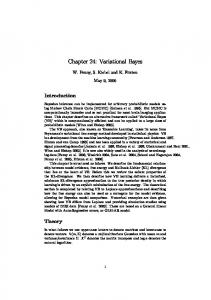
Algorithm 1: VB for LDA Input: Data (nd )D d=1 ; hyperparameters η, α Output: λ Initialize λ while (λ, γ, φ) not converged do for d = 1, . . . , D do (γd , φd ) ← LocalVB(d, λ) PD ∀(k, v), λkv ← ηkv + d=1 φdvk ndv Subroutine LocalVB(d, λ) Output: (γd , φd ) Initialize γd while (γd , φd ) not converged do ∀(k, v), set φdvk ∝ exp (Eq [log θdk ] + Eq [log βkv ]) (normalized across k) PV ∀k, γdk ← αk + v=1 φdvk ndv Subroutine 2: SVI for LDA Input: Hyperparameters η, α, D, (ρt )Tt=1 Output: λ Initialize λ for t = 1, . . . , T do Collect new data minibatch C foreach document indexed d in C do (γd , φd ) ← LocalVB(d, λ) ˜ kv ← ηkv + D P ∀(k, v), λ φdvk ndv |C|

d in C

˜ kv ∀(k, v), λkv ← (1 − ρt )λkv + ρt λ Subroutine 3: SSU for LDA Input: Hyperparameters η, α Output: A sequence λ(1) , λ(2) , . . . (0) Initialize ∀(k, v), λkv ← ηkv for b = 1, 2, . . . do Collect new data minibatch C foreach document indexed d in C do (γd , φd ) ← LocalVB(d, λ) P (b) (b−1) ∀(k, v), λkv ← λkv + d in C φdvk ndv Figure 1: Algorithms for calculating λ, the parameters for the topic posteriors in LDA. VB iterates multiple times through the data, SVI makes a single pass, and SSU is streaming. Here, ndv represents the number of words v in document d.

6

Mean-field variational Bayes. We use the shorthand pD for Eq. (7), the posterior given D documents. We assume the approximating distribution, written qD for shorthand, takes the form qD (β, θ, z | λ, γ, φ) "K # "D # "D N # d Y Y YY = qD (βk | λk ) · qD (θd | γd ) · qD (zdn | φdwdn ) k=1

(8)

d=1 n=1

d=1

for parameters (λkv ), (γdk ), (φdvk ) with k ∈ {1, . . . , K}, v ∈ {1, . . . , V }, d ∈ {1, . . . , D}. Moreover, we set qD (βk | λk ) = DirichletV (βk | λk ), qD (θd | γd ) = DirichletK (θd | γd ), and qD (zdn | φdwdn ) = CategoricalK (zdn | φdwdn ). The subscripts on Dirichlet and Categorical indicate the dimensions of the distributions (and of the parameters). The problem of VB is to find the best approximating qD , defined as the collection of variational parameters λ, γ, φ that minimize the KL divergence from the true posterior: KL (qD k pD ). Even finding the minimizing parameters is a difficult optimization problem. Typically the solution is approximated by coordinate descent in each parameter [6, 13] as in Alg. 1. The derivation of VB for LDA can be found in [4, 13] and Sup. Mat. A.1. Expectation propagation. An EP [7] algorithm for approximating the LDA posterior appears in Alg. 6 of Sup. Mat. B. Alg. 6 differs from [14], which does not provide an approximate posterior for the topic parameters, and is instead our own derivation. Our version of EP, like VB, learns factorized Dirichlet distributions over topics.

3.2

Other single-pass algorithms for approximate LDA posteriors

The algorithms in Sec. 3.1 pass through the data multiple times and require storing the data set in memory—but are useful as primitives for SDA-Bayes in the context of the processing of minibatches of data. Next, we consider two algorithms that can pass through a data set just one time (single pass) and to which we compare in the evaluations (Sec. 4). Stochastic variational inference. VB uses coordinate descent to find a value of qD , Eq. (8), that locally minimizes the KL divergence, KL (qD k pD ). Stochastic variational inference (SVI) [3, 4] is exactly the application of a particular version of stochastic gradient descent to the same optimization problem. While stochastic gradient descent can often be viewed as a streaming algorithm, the optimization problem itself here depends on D via pD , the posterior on D data points. We see that, as a result, D must be specified in advance, appears in each step of SVI (see Alg. 2), and is independent of the number of data points actually processed by the algorithm. Nonetheless, while one may choose to visit D0 6= D data points or revisit data points when using SVI to estimate pD [3, 4], SVI can be made single-pass by visiting each of D data points exactly once and then has constant memory requirements. We also note that two new parameters, τ0 > 0 and κ ∈ (0.5, 1], appear in SVI, beyond those in VB, to determine a learning rate ρt as a function of iteration t: ρt := (τ0 + t)−κ . Sufficient statistics. On each round of VB (Alg. 1), update the local paramePwe D ters for all documents and then compute λkv ← ηkv + d=1 φdvk ndv . An alternative 7

single-pass (and indeed streaming) option would be to update the local parameters for each minibatch of documents as they arrive and then add the corresponding terms φdvk ndv to the current estimate of λ for each document d in the minibatch. This essential idea has been proposed previously for models other than LDA by [11, 12] and forms the basis of what we call the sufficient statistics update algorithm (SSU): Alg. 3. This algorithm is equivalent to SDA-Bayes with A chosen to be a single iteration over the global variable λ of VB (i.e., updating λ exactly once instead of iterating until convergence).

4

Evaluation

We follow [4] (and further [15, 16]) in evaluating our algorithms by computing (approximate) predictive probability. Under this metric, a higher score is better, as a better model will assign a higher probability to the held-out words. We calculate predictive probability by first setting aside held-out testing documents C (test) from the full corpus and then further setting aside a subset of held-out testing words Wd,test in each testing document d. The remaining (training) documents C (train) are used to estimate the global parameter posterior q(β), and the remaining (training) words Wd,train within the dth testing document are used to estimate the documentspecific parameter posterior q(θd ).1 To calculate predictive probability, an approximation is necessary since we do not know the predictive distribution—just as we seek to learn the posterior distribution. Specifically, we calculate the normalized predictive distribution and report “log predictive probability” as P (train) , Wd,train ) d∈C (test) log p(Wd,test | C P d∈C (test) |Wd,test | P P (train) , Wd,train ) d∈C (test) wtest ∈Wd,test log p(wtest | C P , = d∈C (test) |Wd,test | where we use the approximation p(wtest | C (train) , Wd,train ) ! Z Z K X = θdk βkwtest p(θd | Wd,train , β) p(β | C (train) ) dθd dβ β

θd

Z Z ≈ β

θd

k=1 K X

! θdk βkwtest

q(θd ) q(β) dθd dβ =

k=1

K X

Eq [θdk ] Eq [βkwtest ].

k=1

To facilitate comparison with SVI, we use the Wikipedia and Nature corpora of [3, 5] in our experiments. These two corpora represent a range of sizes (3,611,558 training documents for Wikipedia and 351,525 for Nature) as well as different types of topics. We expect words in Wikipedia to represent an extremely broad range of topics 1 In all cases, we estimate q(θ ) for evaluative purposes using VB since direct EP estimation takes d prohibitively long.

8

Wikipedia Log pred prob Time (hours)

Nature

32-SDA

1-SDA

SVI

SSU

32-SDA

1-SDA

SVI

SSU

−7.31 2.09

−7.43 43.93

−7.32 7.87

−7.91 8.28

−7.11 0.55

−7.19 10.02

−7.08 1.22

−7.82 1.27

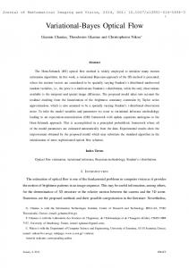
Table 1: A comparison of (1) log predictive probability of held-out data and (2) running time of four algorithms: SDA-Bayes with 32 threads, SDA-Bayes with 1 thread, SVI, and SSU. whereas we expect words in Nature to focus more on the sciences. We further use the vocabularies of [3, 5] and SVI code available online at [17]. We hold out 10,000 Wikipedia documents and 1,024 Nature documents (not included in the counts above) for testing. In the results presented in the main text, we follow [3, 4] in fitting an LDA model with K = 100 topics and hyperparameters chosen as: ∀k, αk = 1/K, ∀(k, v), ηkv = 0.01. For both Wikipedia and Nature, we set the parameters in SVI according to the optimal values of the parameters described in Table 1 of [3] (number of documents D correctly set in advance, step size parameters κ = 0.5 and τ0 = 64). Figs. 3(a) and 3(b) demonstrate that both SVI and SDA are sensitive to minibatch size when ηkv = 0.01, with generally superior performance at larger batch sizes. Interestingly, both SVI and SDA performance improve and are steady across batch size when ηkv = 1 (Figs. 3(a) and 3(b)). Nonetheless, we use ηkv = 0.01 in what follows in the interest of consistency with [3, 4]. Moreover, in the remaining experiments, we use a large minibatch size of 215 = 32,768. This size is the largest before SVI performance degrades in the Nature data set (Fig. 3(b)). Performance and timing results are shown in Table 1. One would expect that with additional streaming capabilities, SDA-Bayes should show a performance loss relative to SVI. We see from Table 1 that such loss is small in the single-thread case, while SSU performs much worse. SVI is faster than single-thread SDA-Bayes in this single-pass setting. Full SDA-Bayes improves run time with no performance cost. We handicap SDA-Bayes in the above comparisons by utilizing just a single thread. In Table 1, we also report performance of SDA-Bayes with 32 threads and the same minibatch size. In the synchronous case, we consider minibatch size to equal the total number of data points processed per round; therefore, the minibatch size equals the number of data points sent to each thread per round times the total number of threads. In the asynchronous case, we analogously report minibatch size as this product. Fig. 2 shows the performance of SDA-Bayes when we run with {1, 2, 4, 8, 16, 32} threads while keeping the minibatch size constant. The goal in such a distributed context is to improve run time while not hurting performance. Indeed, we see dramatic run time improvement as the number of threads grows and in fact some slight performance improvement as well. We tried both a parallel version and a full distributed, asynchronous version of the algorithm; Fig. 2 indicates that the speedup and performance improvements we see here come from parallelizing—which is theoretically justified by Eq. (3) when A is Bayes rule. Our experiments indicate that our Hogwild!-style

9

log predictive probability

log predictive probability

sync async

−7.3 −7.35 −7.4 −7.45 1

−7.1 −7.15 −7.2

2 4 8 16 32 number of threads

1

(a) Wikipedia

run time (hours)

run time (hours)

20 10 1

2 4 8 16 number of threads

sync async

10

30

0

2 4 8 16 32 number of threads (b) Nature

sync async

40

sync async

8 6 4 2 0

32

(c) Wikipedia

1

2 4 8 16 number of threads

32

(d) Nature

Figure 2: SDA-Bayes log predictive probability (two upper plots) and run time (two lower plots) as a function of number of threads. asynchrony does not hurt performance. In our experiments, the processing time at each thread seems to be approximately equal across threads and dominate any communication time at the master, so synchronous and asynchronous performance and running time are essentially identical. In general, a practitioner might prefer asynchrony since it is more robust to node failures. SVI is sensitive to the choice of total data size D. The evaluations above are for a single posterior over D data points. Of greater concern to us in this work is the evaluation of algorithms in the streaming setting. We have seen that SVI is designed to find the posterior for a particular, pre-chosen number of data points D. In practice, when we run SVI on the full data set but change the input value of D in the algorithm, we can see degradations in performance. In particular, we try values of D equal to {0.01, 0.1, 1, 10, 100} times the true D in Fig. 3(c) for the Wikipedia data set and in Fig. 3(d) for the Nature data set. A practitioner in the streaming setting will typically not know D in advance, or multiple values of D may be of interest. Figs. 3(c) and 3(d) illustrate that an estimate may not be sufficient. Even in the case where D is known in advance, it is reasonable to imagine a new influx of further data. One might need to run SVI again from the start

10

(and, in so doing, revisit the first data set) to obtain the desired performance. SVI is sensitive to learning step size. [3, 5] use cross-validation to tune step-size parameters (τ0 , κ) in the stochastic gradient descent component of the SVI algorithm. This cross-validation requires multiple runs over the data and thus is not suited to the streaming setting. Figs. 3(e) and 3(f) demonstrate that the parameter choice does indeed affect algorithm performance. In these figures, we keep D at the true training data size. [3] have observed that the optimal (τ0 , κ) may interact with minibatch size, and we further observe that the optimal values may vary with D as well. We also note that recent work has suggested a way to update (τ0 , κ) adaptively during an SVI run [18]. EP is not suited to LDA. Earlier attempts to apply EP to the LDA model in the non-streaming setting have had mixed success, with [19] in particular finding that EP performance can be poor for LDA and, moreover, that EP requires “unrealistic intermediate storage requirements.” We found this to also be true in the streaming setting. We were not able to obtain competitive results with EP; based on an 8-thread implementation of SDA-Bayes with an EP primitive2 , after over 91 hours on Wikipedia (and 6.7 × 104 data points), log predictive probability had stabilized at around −7.95 and, after over 97 hours on Nature (and 9.7 × 104 data points), log predictive probability had stabilized at around −8.02. Although SDA-Bayes with the EP primitive is not effective for LDA, it remains to be seen whether this combination may be useful in other domains where EP is known to be effective.

5

Discussion

We have introduced SDA-Bayes, a framework for streaming, distributed, asynchronous computation of an approximate Bayesian posterior. Our framework makes streaming updates to the estimated posterior according to a user-specified approximation primitive. We have demonstrated the usefulness of our framework, with variational Bayes as the primitive, by fitting the latent Dirichlet allocation topic model to the Wikipedia and Nature corpora. We have demonstrated the advantages of our algorithm over stochastic variational inference and the sufficient statistics update algorithm, particularly with respect to the key issue of obtaining approximations to posterior probabilities based on the number of documents seen thus far, not posterior probabilities for a fixed number of documents. Acknowledgments We thank M. Hoffman, C. Wang, and J. Paisley for discussions, code, and data and our reviewers for helpful comments. TB is supported by the Berkeley Fellowship, NB by a Hertz Foundation Fellowship, and ACW by the Chancellor’s Fellowship at UC Berkeley. This research is supported in part by NSF CISE Expeditions award CCF-1139158, DARPA XData Award FA8750-12-2-0331, and AMPLab sponsor donations from Amazon Web Services, Google, SAP, Blue Goji, Cisco, Clearstory Data, 2 We chose 8 threads since any fewer was too slow to get results and anything larger created too high of a memory demand on our system.

11

log predictive probability

log predictive probability

−7 −7.3 −7.6 −7.9 SVI, η = 1.0 SVI, η = 0.01 SDA, η = 1.0 SDA, η = 0.01

−8.2 −8.5

5

10 15 log batch size (base 2)

−7.3 −7.35 −7.4 −7.45 −7.5 0

D = 361155800 D = 36115580 D = 3611558 D = 361155 D = 36115

1e6 2e6 3e6 number of examples seen

log predictive probability

log predictive probability

−7.35 −7.4

−7.5 0

−7.9 SDA, η = 1.0 SDA, η = 0.01 SVI, η = 0.01 SVI, η = 1.0

−8.2 −8.5

5

10 15 log batch size (base 2)

−7 −7.2 −7.4 −7.6 D = 3515250 D = 35152500 D = 351525 D = 35152 D = 3515

−7.8 −8

1e5 2e5 3e5 number of examples seen

(d) SVI sensitivity to D on Nature

−7.3

−7.45

−7.6

0

(c) SVI sensitivity to D on Wikipedia

τ0 τ0 τ0 τ0 τ0 τ0

−7.3

(b) Sensitivity to minibatch size on Nature

log predictive probability

log predictive probability

(a) Sensitivity to minibatch size on Wikipedia

−7

= 16, κ = 1.0 = 256, κ = 0.5 = 64, κ = 1.0 = 256, κ = 1.0 = 64, κ = 0.5 = 16, κ = 0.5

1e6 2e6 3e6 number of examples seen

(e) SVI sensitivity to stepsize parameters on Wikipedia

−7 −7.2 −7.4 −7.6 −7.8 −8 0

τ0 τ0 τ0 τ0 τ0 τ0

= 16, κ = 0.5 = 64, κ = 0.5 = 256, κ = 1.0 = 16, κ = 1.0 = 64, κ = 1.0 = 256, κ = 0.5

1e5 2e5 3e5 number of examples seen

(f) SVI sensitivity to stepsize parameters on Nature

Figure 3: Sensitivity of SVI and SDA-Bayes to some respective parameters. Legends have the same top-to-bottom order as the rightmost curve points.

12

Cloudera, Ericsson, Facebook, General Electric, Hortonworks, Intel, Microsoft, NetApp, Oracle, Samsung, Splunk, VMware and Yahoo!. This material is based upon work supported in part by the Office of Naval Research under contract/grant number N00014-11-1-0688.

References [1] F. Niu, B. Recht, C. R´e, and S. J. Wright. Hogwild!: A lock-free approach to parallelizing stochastic gradient descent. In Neural Information Processing Systems, 2011. [2] A. Kleiner, A. Talwalkar, P. Sarkar, and M. Jordan. The big data bootstrap. In International Conference on Machine Learning, 2012. [3] M. Hoffman, D. M. Blei, and F. Bach. Online learning for latent Dirichlet allocation. In Neural Information Processing Systems, volume 23, pages 856–864, 2010. [4] M. Hoffman, D. M. Blei, J. Paisley, and C. Wang. Stochastic variational inference. Journal of Machine Learning Research, 14:1303–1347. [5] C. Wang, J. Paisley, and D. M. Blei. Online variational inference for the hierarchical Dirichlet process. In Artificial Intelligence and Statistics, 2011. [6] M. J. Wainwright and M. I. Jordan. Graphical models, exponential families, and variational inference. Foundations and Trends in Machine Learning, 1(1-2):1–305, 2008. [7] T. P. Minka. Expectation propagation for approximate Bayesian inference. In Uncertainty in Artificial Intelligence, pages 362–369. Morgan Kaufmann, 2001. [8] T. P. Minka. A family of algorithms for approximate Bayesian inference. PhD thesis, Massachusetts Institute of Technology, 2001. [9] M. Opper. A Bayesian approach to on-line learning. [10] K. R Canini, L. Shi, and T. L Griffiths. Online inference of topics with latent Dirichlet allocation. In Artificial Intelligence and Statistics, volume 5, 2009. [11] A. Honkela and H. Valpola. On-line variational Bayesian learning. In International Symposium on Independent Component Analysis and Blind Signal Separation, pages 803–808, 2003. [12] J. Luts, T. Broderick, and M. P. Wand. Real-time semiparametric regression. Journal of Computational and Graphical Statistics, to appear. Preprint arXiv:1209.3550. [13] D. M. Blei, A. Y. Ng, and M. I. Jordan. Latent Dirichlet allocation. Journal of Machine Learning Research, 3:993–1022, 2003. [14] T. Minka and J. Lafferty. Expectation-propagation for the generative aspect model. In Uncertainty in Artificial Intelligence, pages 352–359. Morgan Kaufmann, 2002. [15] Y. Teh, D. Newman, and M. Welling. A collapsed variational Bayesian inference algorithm for latent Dirichlet allocation. In Neural Information Processing Systems, 2006. [16] A. Asuncion, M. Welling, P. Smyth, and Y. Teh. On smoothing and inference for topic models. In Uncertainty in Artificial Intelligence, 2009.

13

[17] M. Hoffman. Online inference for LDA (Python code) at http://www.cs.princeton.edu/˜blei/downloads/onlineldavb.tar, 2010. [18] R. Ranganath, C. Wang, D. M. Blei, and E. P. Xing. An adaptive learning rate for stochastic variational inference. In International Conference on Machine Learning, 2013. [19] W. L. Buntine and A. Jakulin. Applying discrete PCA in data analysis. In Uncertainty in Artificial Intelligence. [20] M. Seeger. Expectation propagation for exponential families. Technical report, University of California at Berkeley, 2005.

14

A A.1

Variational Bayes Batch VB

As described in the main text, the idea of VB is to find the distribution qD that best approximates the true posterior, pD . More specifically, the optimization problem of VB is defined as finding a qD to minimize the KL divergence between the approximating distribution and the posterior: KL (qD k pD ) := EqD [log (qD /pD )] Typically qD takes a particular, constrained form, and finding the optimal qD amounts to finding the optimal parameters for qD . Moreover, the optimal parameters usually cannot be expressed in closed form, so often a coordinate descent algorithm is used. For the LDA model, we have qD in the form of Eq. (8) and pD defined by Eq. (7). We wish to find the following variational parameters (i.e., parameters to qD ): λ (describing each topic), γ (describing the topic proportions in each document), and φ (describing the assignment of each word in each document to a topic). A.1.1

Evidence lower bound

Finding qD to minimize the KL divergence between qD and pD is equivalent to finding qD to maximize the evidence lower bound (ELBO), ELBO := EqD [log p(Θ, x1:D )] − EqD [log qD ] = EqD [log pD ] + p(x1:D ) − EqD [log qD ] = −KL (qD k pD ) + p(x1:D ), since p(x1:D ) is constant in qD . The VB optimization problem is often phrased in terms of the ELBO instead of the KL divergence. The ELBO for LDA can be written as follows, where the model parameters are β, θ, z and the data is w; η and α are fixed hyperparameters. ELBO(λ, γ, φ) = Eq [log p(β, θ, z, w | η, α)] − Eq [log q(β, θ, z | λ, γ, φ)] =

K X

Eq [log Dirichlet(βk | ηk )] +

k=1

+

D X

Eq [log Dirichlet(θd | α)]

d=1 Nd D X X

Eq [log Multinomial(zdn | θd )] +

d=1 n=1

−

K X

Eq [log Dirichlet(βk | λk )] −

Nd D X X

Eq [log Multinomial(wdn | βzdn )]

d=1 n=1

k=1

−

Nd D X X

D X

Eq [log Dirichlet(θd | γd )]

d=1

Eq [log Multinomial(zdn | φdwdn )] .

d=1 n=1

15

The expectations in q in the previous equation can be evaluated as follows. The equations below make use of the digamma function ψ and trigamma function ψ1 . Here,   d d ψ(x) = log Γ(x) = Γ(x) /Γ(x) dx dx d d2 ψ1 (x) = 2 log Γ(x) = ψ(x). dx dx Then, Eq [log Dirichlet(βk | ηk )] ! V V V X X X = log Γ ηkv − log Γ(ηkv ) + (ηkv − 1) Eq [log βkv ] v=1

= log Γ

V X

v=1

! ηkv

−

v=1

V X

v=1 V V X  X log Γ(ηkv ) + (ηkv − 1) ψ(λkv ) − ψ λku

v=1

v=1

u=1

Eq [log Dirichlet(θd | α)] ! K K K X X X = log Γ αk − log Γ(αk ) + (αk − 1) Eq [log θdk ] k=1

= log Γ

K X

! αk

k=1

−

k=1

k=1

K X

K X

log Γ(αk ) +

k=1

 (αk − 1) ψ(γdk ) − ψ

K X j=1

k=1

Eq [log Multinomial(zdn | θd )] =

K X

φdwdn k Eq [log θdk ]

k=1

=

K X

 φdwdn k ψ(γdk ) − ψ

K X

 

γdj 

j=1

k=1

Eq [log Multinomial(wdn | βzdn )] =

V X

1{wdn = v} Eq [log βzdn ,v ]

v=1

=

V X

1{wdn = v}

v=1

=

K X

φdwdn k Eq [log βkv ]

k=1

V X K X

1{wdn = v} φdwdn k ψ(λkv ) − ψ

v=1 k=1

V X

λku



!

u=1

Eq [log Dirichlet(βk | λk )] ! V V V X X X = log Γ λkv − log Γ(λkv ) + (λkv − 1) Eq [log βkv ] v=1

v=1

v=1

16

 

γdj 

!

= log Γ

V X

! −

λkv

v=1

V X

V V X  X log Γ(λkv ) + (λkv − 1) ψ(λkv ) − ψ λku

v=1

v=1

!

u=1

Eq [log Dirichlet(θd | γd )] ! K K K X X X = log Γ γdk − log Γ(γdk ) + (γdk − 1) Eq [log θdk ] k=1

= log Γ

K X

! γdk

−

k=1

k=1

k=1

K X

K X

log Γ(γdk ) +

k=1

 (γdk − 1) ψ(γdk ) − ψ

K X

 

γdj 

j=1

k=1

Eq [log Multinomial(zdn | φdn )] =

K X

φdwdn k log φdwdn k .

k=1

A.1.2

Coordinate ascent

We maximize the ELBO via coordinate ascent in each dimension of the variational parameters: λ, γ, and φ. Variational parameter λ. Choose a topic index k. Fix γ, φ, and each λj for j 6= k. Then we can write the ELBO’s functional dependence on λk as follows, where “const” is a constant in λk . ! V V X  X ELBO(λk ) = (ηkv − 1) ψ(λkv ) − ψ λku v=1

+

u=1 Nd X V D X X

1{wdn = v} φdwdn k ψ(λkv ) − ψ

− log Γ

! λkv

+

v=1

V X

log Γ(λkv )

ηkv − λkv +

v=1

− log Γ

! + const

u=1

v=1

=

!

v=1

V V X  X λku (λkv − 1) ψ(λkv ) − ψ − V X

λku



u=1

d=1 n=1 v=1 V X

V X

Nd D X X

1{wdn = v} φdwdn k

!

d=1 n=1 V X v=1

! λkv

+

ψ(λkv ) − ψ

V X

λku

u=1

V X

log Γ(λkv ) + const

v=1

The partial derivative of ELBO(λk ) with respect to one of the dimensions of λk , say λkv , is ∂ ELBO(λk ) ∂λkv 17

! 

= − ψ(λkv ) − ψ

V X

λku



!

u=1

ηkv − λkv +

+

Nd D X X

1{wdn = v} φdwdn k

! ψ1 (λkv ) − ψ1

d=1 n=1

X

−

= ψ1 (λkv )

1{wdn = t} φdwdn k

! ψ1

d=1 n=1

t:t6=v

Nd D X X

ηkv − λkv +

λku



!

u=1

Nd D X X

ηkt − λkt +

V X

V X

V  X  λku − ψ λku + ψ(λkv )

u=1

1{wdn = v} φdwdn k

u=1

!

d=1 n=1

−ψ

V X

λku

V  X

u=1

ηku − λku +

u=1

Nd D X X

!

1{wdn = u} φdwdn k .

d=1 n=1

From the last line of the previous equation, we see that one can set the gradient of ELBO(λk ) to zero by setting λkv ← ηkv +

Nd D X X

1{wdn = v} φdwdn k

for v = 1, . . . , V.

d=1 n=1

Equivalently, if ndv is the number of occurrences (tokens) of word type v in document d, then the update may be written λkv ← ηkv +

D X

ndv φdvk

for v = 1, . . . , V.

d=1

Variational parameter γ. Now choose a document d. Fix λ, φ, and γc for c 6= d. Then we can express the functional dependence of the ELBO on γd as follows.     Nd X K K K K X  X  X X γdj  + φdwdn k ψ(γdk ) − ψ γdj  ELBO(γd ) = (αk − 1) ψ(γdk ) − ψ j=1

k=1

− log Γ

K X

! γdk

+

k=1

K X

log Γ(γdk ) −

k=1

n=1 k=1 K X

j=1

 (γdk − 1) ψ(γdk ) − ψ

j=1

k=1

+ const =

K X

αk − γdk +

! φdwdn k

ψ(γdk ) − ψ

K X

n=1

k=1

− log Γ

Nd X

K X k=1

j=1

! γdk

+

K X

log Γ(γdk ) + const

k=1

18

K X

 

γdj 

 

γdj 

The partial derivative of ELBO(γd ) with respect to one of the dimensions of γd , say γdk , is ∂ ELBO(γd ) ∂γdk  = − ψ(γdk ) − ψ

K X

 

αk − γdk +

γdj  +

−

αi − γdi +

Nd X

! φdwdn i

ψ1

K X

n=1

i:i6=k

= ψ1 (γdk ) αk − γdk +

! φdwdn k

ψ1 (γdk ) − ψ1

n=1

j=1

X

Nd X

Nd X



γdj − ψ

φdwdn k

− ψ1

γdj 

K X

 γdj + ψ(γdk )

j=1

K X

n=1



j=1

j=1

!



K X

γdj

K X

j=1

αj − γdj +

j=1

Nd X

! φdwdn j

n=1

As for the λ case above, one obvious way to achieve a gradient of ELBO(γd ) equal to zero is to set Nd X γdk ← αk + φdwdn k for k = 1, . . . , K. n=1

Equivalently, γdk ← αk +

V X

ndv φdvk

for k = 1, . . . , K.

v=1

Variational parameter φ. Finally, consider fixing λ, γ, and φcu for (c, u) 6= (d, v). In this case, the dependence of the ELBO on φdv can be written as follows. ELBO(φdv ) =

K X

 ndv φdvk ψ(γdk ) − ψ

+

K X

ndv φdvk

γdj 

ψ(λkv ) − ψ

V X

λku



! −

u=1

k=1

=

 

j=1

k=1

K X

K X

 ndv φdvk − log φdvk + ψ(γdk ) − ψ

ndv φdvk log φdvk + const

k=1 K X j=1

k=1

K X



γdj + ψ(λkv ) − ψ

V X

 

λku 

u=1

+ const The partial derivative of ELBO(φdv ) with respect to one of the dimensions of φdv , say φdvk , is ∂ ELBO(φdv ) ∂φdvk

19

.

 = ndv − log φdvk + ψ(γdk ) − ψ

K X



γdj + ψ(λkv ) − ψ

V X

 

λku − 1 .

u=1

j=1

Using the method of Lagrange multipliers to incorporate the constraint that 1, we wish to find ρ and φdvk such that " !# K X ∂ ELBO(φdv ) − ρ φdvk − 1 . 0= ∂φdvk

PK

k=1

φdvk =

(9)

k=1

Setting  φdvk ∝k exp ψ(γdk ) − ψ

K X



γdj + ψ(λkv ) − ψ

V X

 

λku 

u=1

j=1

achieves the desired outcome in Eq. (9). Here, ∝k indicates that the proportionality is across k. The optimal choice of ρ is expressed via this proportionality. The above assignment may also be written as φdvk ∝k exp (Eq [log θdk ] + Eq [log βkv ]) The coordinate-ascent algorithm iteratively updates the parameters λ, γ, and φ. In practice, we usually iterate the updates for the “local” parameters φ and γ until they converge, then update the “global” parameter λ, and repeat. The resulting batch variational Bayes algorithm is presented in Alg. 1.

A.2

SDA-Bayes VB

For a fixed hyperparameter α, we can think of BatchVB as an algorithm that takes input in the form of a prior on topic parameters β and a minibatch of documents. In particular, let Cb be the bth minibatch of documents; for documents with indices in Db , these documents can be summarized by the word counts (nd )d∈Db . Then, in the notation of Eq. (2), we have Θ = β, A = BatchVB, and q0 (β) =

K Y

Dirichlet(βk |ηk ).

k=1

In general, the bth posterior takes the same form and therefore can be summarized by its parameters λ(b) : qb (β) =

K Y

(b)

Dirichlet(βk |λk ).

k=1

20

(0)

In this case, if we set the prior parameters to λk following algorithm.

:= ηk , Eq. (2) becomes the

Algorithm 4: Streaming VB for LDA Input: Hyperparameter η Initialize λ(0) ← η foreach Minibatch C b of documents  do λ(b) ← BatchVB Cb , λ(b−1) QK (b) qb (β) = k=1 Dirichlet(βk |λk )

Next, we apply the asynchronous, distributed updates described in the “Asynchronous Bayesian updating” portion of Sec. 2 to the batch VB primitive and LDA model. In this case, λ(post) is the posterior parameter estimate maintained at the master, and each worker updates this value after a local computation. The posterior after seeing a colQK (post) lection of minibatches is q(β) = k=1 Dirichlet(βk |λk ). Algorithm 5: SDA-Bayes with VB primitive for LDA Input: Hyperparameter η Initialize λ(post) ← η foreach Minibatch Cb of documents, at a worker do   Copy master value locally: λ(local) ← λ(post) λ ← BatchVB Cb , λ(local) ∆λ ← λ − λ(local) Update the master value synchronously: λ(post) ← λ(post) + ∆λ

B B.1

Expectation Propagation Batch EP

Our batch expectation propagation (EP) algorithm for LDA learns a posterior for both the document-specific topic mixing proportions (θd )D d=1 and the topic distributions over . By contrast, the algorithm in [14] learns only the former and so is not words (βk )K k=1 appropriate to the model in Sec. 3. For consistency, we also follow [14] in making a distinction between token and type word updates, where a token refers to a particular word instance and a type refers to all words with the same vocabulary value. Let C = (wd )D d=1 denote the set of documents that we observe, and for each word v in the vocabulary, let ndv denote the number of times v appears in document d. Collapsed posterior. We begin by collapsing (i.e., integrating out) the word assignments z in the posterior (7) of LDA. We can express the collapsed posterior as "K # D " !ndv # V K X Y Y Y p(β, θ | C, η, α) ∝ DirichletV (βk | ηk ) · DirichletK (θd | α) · θdk βkv . k=1

d=1

21

v=1

k=1

PK For each document-word pair (d, v), consider approximating the term k=1 θdk βkv above by "K # Y DirichletV (βk | χkdv + 1V ) · DirichletK (θd | ζdv + 1K ), k=1

where χkdv ∈ RV , ζdv ∈ RK , and 1M is a vector of all ones of length M . This proposal serves as inspiration for taking the approximating variational distribution for p(β, θ | C, η, α) to be of the form "K # D Y Y q(β, θ | λ, γ) := q(βk | λk ) · q(θd | γd ), (10) k=1

d=1

where q(βk | λk ) = Dirichlet(βk | λk ) and q(θd | γd ) = Dirichlet(θd | γd ), with the parameters λ k = ηk +

V D X X

ndv χkdv ,

γd = α +

V X

ndv ζdv ,

(11)

v=1

d=1 v=1

and the constraints λk ∈ RV+ and γd ∈ RK + for each k and d. We assume this form in the remainder of the analysis and write q(β, θ | χ, ζ) for q(β, θ | λ, γ), where χ = (χkdv ), ζ = (ζdv ). Optimization problem. We seek to find the optimal parameters (χ, ζ) by minimizing the (reverse) KL divergence: min KL (p(β, θ | C, η, α) k q(β, θ | χ, ζ)) . χ,ζ

This joint minimization problem is not tractable, and the idea of EP is to proceed iteratively by fixing most of the factors in Eq. (10) and minimizing the KL divergence over the parameters related to a single word. More formally, suppose we already have a set of parameters (χ, ζ). Consider a document d and word v that occurs in document d (i.e., ndv ≥ 1). We start by removing the component of q related to (d, v) in Eq. (10). Following [7], we subtract out the effect of one occurrence of word v in document d, but at the end of this process we update the distribution on the type level. In doing so, we use the following shorthand for the remaining global parameters: X \(d,v) λk = λk − χkdv = ηk + (ndv − 1)χkdv + nd0 v0 χkd0 v0 (d0 ,v 0 ):(d0 ,v 0 )6=(d,v) \(d,v)

γd

= γd − ζdv = α + (ndv − 1)ζdv +

X

ndv0 ζdv0 .

v 0 :v 0 6=v

PK We replace this removed part of q by the term k=1 θdk βkv , which corresponds to the contribution of one occurrence of word v in document d to the true posterior p. Call

22

\(d,v)

the resulting normalized distribution q˜dv , so q˜dv (β, θ | λ\(d,v) , γ\d , γd ) satisfies  "K #  K Y Y X \(d,v) \(d,v) ∝ Dirichlet(βk | λk ) · Dirichlet(θd0 | γd0 ) · Dirichlet(θd | γd )· θdk βkv . d0 6=d

k=1

k=1

We obtain an improved estimate of the posterior q by updating the parameters from ˆ γˆ ), where (λ, γ) to (λ,   ˆ γˆ ) = arg min KL q˜dv (β, θ | λ\(d,v) , γ\d , γ \(d,v) ) k q(β, θ | λ0 , γ 0 ) . (λ, (12) d 0 0 λ ,γ

Solution to the optimization problem. First, note that for d0 : d0 6= d, we have γˆd0 = γd0 . Now consider the index d chosen on this iteration. Since β and θ are Dirichletdistributed under q, the minimization problem in Eq. (12) reduces to solving the momentmatching equations [7, 20] Eq˜dv [log βku ] = Eλˆ k [log βku ]

for 1 ≤ k ≤ K, 1 ≤ u ≤ V,

Eq˜dv [log θdk ] = Eγˆd [log θdk ]

for 1 ≤ k ≤ K.

These can be solved via Newton’s method though [7] recommends solving exactly for the first and “average second” moments of βku and θdk , respectively, instead. We choose the latter approach for consistency with [7]; our own experiments also suggested taking the approach of [7] was faster than Newton’s method with no noticeable performance loss. The resulting moment updates are  PV  2 y=1 Eq˜dv [βky ] − Eq˜dv [βky ] ˆ ku =  · Eq˜dv [βku ] (13) λ PV  2 2 y=1 Eq˜dv [βky ] − Eq˜dv [βky ]  PK  2 E [θ ] − E [θ ] q˜dv dj q˜d,n dj j=1   · Eq˜dv [θdk ]. γˆdk = P (14) K 2 2 j=1 Eq˜dv [θdj ] − Eq˜dv [θdj ] K We then set (χkdv )K k=1 and ζdv such that the new global parameters (λk )k=1 and γd are K ˆk ) equal to the optimal parameters (λ ˆd . The resulting algorithm is presented k=1 and γ

23

below (Alg. 6). Algorithm 6: EP for LDA Input: Data C = (wd )D d=1 ; hyperparameters η, α Output: λ Initialize ∀(k, d, v), χkdv ← 0 and ζdv ← 0 while (χ, ζ) not converged do foreach (d, v) with ndv ≥ 1 do /* Variational distribution without the word token (d, v) P \(d,v) ∀k, λk ← ηk + (ndv − 1)χkdv + (d0 ,v0 )6=(d,v) nd0 v0 χkd0 v0 P \(d,v) γd ← α + (ndv − 1)ζdv + v0 6=v ndv0 ζdv0 \(d,v)

*/

\(d,v)

If any of λku or γdk are non-positive, skip updating this (d, v) (†) /* Variational parameters from moment-matching */ ˆ ku from Eq. (13) ∀(k, u), compute λ ∀k, compute γˆdk from Eq. (14) /* Type-level values */  updates to parameter
\(d,v) −1 ˆ −1 ∀k, χkdv ← ndv λk − λk + 1 − ndv χkdv  
\(d,v) −1 ζdv ← ndv γˆd − γd + 1 − n−1 dv ζdv Other χ, ζ remain unchanged /* Global variational parameters PD PV ∀k, λk ← ηk + d=1 v=1 ndv χkdv

*/

The results in the main text (Sec. 4) are reported for Alg. 6. We also tried a slightly modified EP algorithm that makes token-level updates to parameter values, rather than type-level updates. This modified version iterates through each word placeholder in document d; that is, through pairs (d, n) rather than pairs (d, v) corresponding to word values. Since there are always at least as many (d, n) pairs as (d, v) pairs with ndv ≥ 1 (and usually many more of the former), the modified algorithm requires many more iterations. In practice, we find better experimental performance for the modified EP algorithm in terms of log predictive probability as a function of number of data points in the training set seen so far: e.g., leveling off at about −7.96 for Nature vs. −8.02. However, the modified algorithm is also much slower, and still returns much worse results than SDA-Bayes or SVI, so we do not report these results in the main text.3

B.2

SDA-Bayes EP

Putting a batch EP algorithm for LDA into the SDA-Bayes framework is almost identical to putting a batch VB algorithm for LDA into the SDA-Bayes framework. This 3 Here and in the main text we run EP with η = 1. We also tried EP with η = 0.01, but the positivity \(d,v) \(d,v) check for λku and γdk on line (†) in Algorithm 6 always failed and as a result none of the parameters were updated.

24

similarity is to be expected since SDA-Bayes works out of the box with a batch approximation algorithm in the correct form. For a fixed hyperparameter α, we can think of BatchEP as an algorithm (just like BatchVB) that takes input in the form of a prior on topic parameters β and a minibatch of documents. The same setup and notation from Sup. Mat. A.2 applies. In this case, Eq. (2) becomes the following algorithm. Algorithm 7: Streaming EP for LDA Input: Hyperparameter η Initialize λ(0) ← η foreach Minibatch Cb of documents  do λ(b) ← BatchEP Cb , λ(b−1) QK (b) qb (β) = k=1 Dirichlet(βk |λk )

This algorithm is exactly the same as Alg. 4 but with a batch EP primitive instead of a batch VB primitive. Next, we apply the asynchronous, distributed updates described in the “Asynchronous Bayesian updating” portion of Sec. 2 to the batch EP primitive and LDA model. Again, the setup and notation from Sup. Mat. A.2 applies, and we find the following algorithm. Algorithm 8: SDA-Bayes with EP primitive for LDA Input: Hyperparameter η Initialize λ(post) ← η foreach Minibatch Cb of documents, at a worker do   Copy master value locally: λ(local) ← λ(post) λ ← BatchEP Cb , λ(local) ∆λ ← λ − λ(local) Update the master value synchronously: λ(post) ← λ(post) + ∆λ Indeed, the recipe outlined here applies more generally to other primitives besides EP and VB.

25