We present an extension of the variational Bayesian nonlinear state-space model ... than in [1] by using new linearisation [2] and state inference techniques [3].
Variational Bayes for Continuous-Time Nonlinear State-Space Models
Antti Honkela, Matti Tornio, and Tapani Raiko Adaptive Informatics Research Centre, Helsinki University of Technology P.O. Box 5400, FI-02015 TKK, Finland {Antti.Honkela, Matti.Tornio, Tapani.Raiko}@tkk.fi http://www.cis.hut.fi/projects/bayes/
Abstract We present an extension of the variational Bayesian nonlinear state-space model introduced by Valpola and Karhunen in 2002 [1] for continuous-time models. The model is based on using multilayer perceptron (MLP) networks to model the nonlinearities. Moving to continuous-time requires solving a stochastic differential equation (SDE) to evaluate the predictive distribution of the states, but otherwise all computation happens as in the discrete-time case. The close connection between the methods allows utilising our new improved state inference method for both discrete-time and continuous-time modelling.
1 Introduction The two major types of dynamical systems are discrete time systems modelled with difference equations and continuous-time systems modelled with differential equations. Much of machine learning research in dynamical systems and time series has focused on the the discrete time case because it is often easier to handle. The restriction is often not too severe as regularly sampled continuous-time systems can be modelled as discrete time systems at the sample times. Not all data sets are, however, regularly sampled and often it would be convenient to know what happens between the sample times, hence the need for continuous-time models. The variational Bayesian nonlinear state-space model introduced by Valpola and Karhunen in [1] uses a general nonlinear state-space model for the observations x(t) s(t + 1) = s(t) + gdt (s(t), θ g ) + m(t) x(t) = f (s(t), θ f ) + n(t)
(1) (2)
with states s(t), Gaussian innovation m and noise n, and multi-layer perceptron (MLP) networks to model the nonlinearities f and gdt . Inference and learning in the model can be made more reliable and efficient than in [1] by using new linearisation [2] and state inference techniques [3]. In this work we outline an extension of the model for continuous-time systems along with preliminary experimental results. The method can effectively utilise new developments for the discrete-time case, such as the improved state inference method [3], which is presented as well.
2 Continuous-time nonlinear state-space model The general formulation of the state evolution in a continuous-time nonlinear state-space model is given by a stochastic differential equation (SDE) √ ds = g(s)dt + ΣdW, (3)
where dW is the differential of a Wiener process [4]. The continuous-time nonlinear state-space model is obtained by using Eq. (3) to model state evolution instead of Eq. (1). The nonlinear mapping g is again modelled by a MLP network. The observation equation Eq. (2) remains unchanged.
3 Variational learning Variational Bayesian learning is based on approximating the posterior distribution p(θ, S|X, H) with a tractable approximation q(θ, S|ξ), where X = {x(ti )|i = 1, . . . , N } is the data, S = {s(ti )|i = 1, . . . , N } are the latent state values at the times of the observations, θ are the parameters of the model H, and ξ are the (variational) parameters of the approximation. The approximation is fitted by maximising a lower bound on marginal log-likelihood � � p(X, S, θ|H) = log p(X|H) − DKL (q(S, θ|ξ)||p(S, θ|X, H)), (4) B = log q(S, θ|ξ) where h·i denotes expectation over q. This is equivalent to minimising the Kullback–Leibler DKL (q||p) divergence between q and p [5, 6]. The nonlinear state-space model is learned by numerically maximising the bound (4) with a conjugate gradient method. This requires evaluating the value of the bound and its gradient with respect to all the variational parameters ξ. Given a Gaussian approximation similar to the one used in [1], the most difficult part is to evaluate the expectation hlog p(S|θ)i = hlog p(s(t1 )|θ)i +
N X i=2
hlog p(s(ti )|s(ti−1 )θ)i ,
(5)
where the Markov property of the state sequence has been used. Because a Gaussian variational approximation is used, only the mean and variance of s are needed to evaluate the bound for the continuous-time model. Writing the differential equations for the mean and covariance of a corresponding Gaussian process s satisfying Eq. (3) and using a first order Taylor approximation of g about the mean of s yields two separate equations for the mean µ(t) and covariance P(t) of s as d µ(t) = g(µ(t)) dt
� d P(t) = hG(µ(t))i PT (t) + P(t) GT (µ(t)) + Σ, dt
(6) (7)
where G denotes the Jacobian matrix of g [7]. The expected value of g and the expected Jacobian are evaluated using the linearisation technique presented in [2]. These equations can be solved numerically using a simple Euler method to find required statistics of p(s(ti+1 )|s(ti )). Eq. (6) yields the posterior mean and variance of the predicted mean of s(ti+1 ) that correspond to the mean and variance of gdt (s(t)) in the discrete-time case. Eq. (7), in turn, yields the expected covariance of p(s(ti+1 )|s(ti )), corresponding to the expected covariance of the innovation process m(t) in the discrete-time case. The main difference here is that the covariance of the predictive distribution arises from the process and not from simple additive Gaussian noise. When a simple Euler method is used, gradients of the cost with respect to the variational parameters governing the distributions of the network weights and the state values can be derived from the prediction equations in a similar manner as in the discrete-time case. All these parameters are updated using the same conjugate-gradient algorithm as in the discrete-time case. Higher order parameters such as the number of hidden units in the MLP networks are optimised by comparing the marginal likelihood values resulting from runs with different values, but more automated methods like automatic relevance determination could easily be used as well.
4 State inference Variational Bayesian inference of the state S happens by maximising B in Eq. (4). Doing this directly with a gradient or a conjugate gradient method leads to suboptimal performance. This is because the terms in B that depend on a particular s(t) include only the neighbouring states in time. Information spreads around slowly because the states of different time slices affect each other only between updates. Variants of the Kalman smoother propagate information very fast, but we have found the lack of convergence prohibitive in some cases. In [3], we proposed a novel update algorithm for the posterior means s(t). The marginal posterior approximation is Gaussian s(t))) , q(s(t) | ξ) = N (s(t); s(t), diag(e
(8)
where diag(e s(t)) is a diagonal covariance matrix. We replaced partial derivatives of B w.r.t. state means s(t) for each t = 1, . . . , T by (approximated) total derivatives: T
X ∂B ∂s(τ ) dB = . ds(t) τ =1 ∂s(τ ) ∂s(t)
(9)
The approximation involves linearising the nonlinear mappings around the current state estimates. Assuming linearisations, the optimal state mean sopt (t) as a function of neighbouring state means can be solved analytically1 , but we are especially interested in the dependencies: ∂sopt (t) = diag(e s(t))Σ−1 m Jg (t − 1) ∂s(t − 1) ∂sopt (t) −1 = diag(e s(t))JT g (t)Σm , ∂s(t + 1)
(10) (11)
where Jg is the linearisation matrix [2] of the mapping g and Σm is the noise covariance for m(t) in Eq. (1). The total derivative is then computed by propagating the gradient forward and backward through time assuming these dependencies. The computational overhead turns out to be rather small. Generalisation of the method to the continuous-time case is obvious with proper interpretations of Jg and Σm as the product of the corresponding Jacobians G for each step in the solution of Eq. (6) and as the proper value of P(ti ), respectively.
5 Experiments 5.1 Continuous-time NSSM The continuous-time NSSM is demonstrated with a data set generated by a Lorenz process [8]. A Lorenz process has a three-dimensional state-space with non-linear chaotic dynamics determined by the following set of differential equations: dz1 = σ(z1 − z2 ) dt dz2 = ρz1 − z2 − z1 z3 dt dz3 = z1 z2 − βz3 . dt
(12) (13) (14)
The parameter vector [σ, ρ, β] used in this experiment was [3, 26.5, 1]. The data set was generated by unevenly sampling the process at random time instants between 0 and 20. A data set with 201 samples was used, and the data was normalised to mean of 0 and standard deviation of 1. Additive Gaussian observation noise with a standard deviation of 0.2 was added to the data set. To make learning more challenging and to demonstrate the benefits of the latent statespace, only the two first components of the observations, z1 and z2 , were used in this experiment. 1
See [3] for derivation.
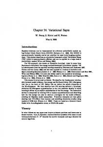
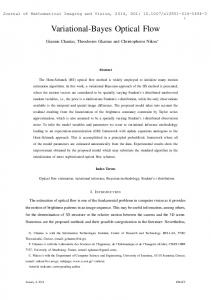
A three dimensional state-space was used to learn this data set. The MLPs for both the observation and the dynamical mapping had 10 hidden units. The original three-dimensional Lorenz process and the three-dimensional state-space can be seen in Fig. 1. Noiseless and noisy versions of the two-dimensional data set used to train the model and the reconstructions of this data set can be seen in Fig. 2. The latent states and their values predicted from the previous state are plotted against time in Fig. 3. The presented results are still preliminary, as the size of the data set used in this experiment is not large enough to properly form the correct state-space or to reliably predict even the short term behavior of the Lorenz process beyond a few time steps. However, the state-space representation was still able to capture the original three-dimensional nature of the Lorenz process using only the two observed data components.
50
2
0 0
−50 10
−2 −2
5 0
0
−5
4
−40
2
−20
−10
2 0
0 −15 20
4 −2
Figure 1: Left: The original three-dimensional Lorenz process without noise. Right: The threedimensional latent state-space of the model.
2
2
2
0
0
0
−2
−2
−2
−4 −4
−2
0
2
−4 −4
−2
0
2
−4 −4
−2
0
2
Figure 2: Left: The original data set without noise. Middle: The noisy data set used in the experiment. Right: The reconstruction of the data set by the model.
2 0 −2 0
20
2 0 −2 0
20
Figure 3: Top: The latent state values. Bottom: The values predicted from the previous time step. The tick marks on the x-axis correspond to sampling instants.
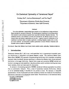
5.2 State inference The presented state inference was tested on a real world data set of speech spectra [3]. The data set consisted of 11200 21 dimensional samples which corresponds to 90 seconds of continuous human speech. The first 10000 samples were used to train a seven dimensional discrete-time state-space model and the rest of the data was used in the experiments. The test data set was divided into three parts each consisting of 300 samples and all the algorithms were run for each data set with four random initialisations. The final results represent an average over both the different data sets and initialisations. Since the true state is unknown, the mean square error of the reconstruction of missing data was used to compare the different algorithms. Experiments were done with sets of both 3 and 30 consecutive missing samples. The ability to cope with missing values is very important when only partial observations are available or in the case of failures in the observation process. It also has interesting applications in the field of control as reported in [9]. The results can be seen in Fig. 4. When large gaps of missing values are present, the proposed algorithm (NDFA+TD) performs clearly better than the rest of the compared algorithms. The compared methods of iterated extended Kalman smoother (IEKS) [10] and iterated unscented Kalman smoother (IUKS) [11,12] had some stability problems and neither of these methods could cope very well with long gaps of missing values.
6 Discussion Solving the differential equations governing state evolution requires finding a suitable discretisation of time. Finer discretisation provides more accuracy, but risks instability when the model of the dynamics is still poor. An adaptive scheme starting with long time steps and decreasing the step length as the model gets more reliable would most likely be very useful in learning problems with larger time gaps.
5 10 15 20
5 10 15 20 50
100
150 sample
200
250
50
300
120
200
250
300
NDFA + TD IEKS IUKS NDFA
220 RMSE
100 RMSE
150 sample
230 NDFA + TD IEKS IUKS NDFA
110
90 80
210 200 190
70 60
100
0
20
40
60 time s
80
100
180
0
50
100 time s
150
200
Figure 4: Inference with the speech data with missing values. On the top one of the data sets used in the experiments (missing values marked in black), on the bottom root mean square error plotted against computation time. Left side figures use a small gap size, right side figures a large gap size. (From [3].)
By moving from discrete time to a continuous-time framework, one can more easily model phenomena that have vastly different time scales. It would be an interesting extension to factor the state s into two (or more) parts s1 and s2 where it is a priori known that the dynamics of s1 are slow compared to the dynamics of s2 . The SDE can be factored into: p ds1 = g1 (s1 )dt + Σ1 dW (15) p (16) ds2 = g2 (s1 , s2 )dt + Σ2 dW, where one should note that the slow part s1 affects the dynamics of the fast part s2 directly but not the other way around. Such a model could in some cases be learned by first learning g1 with more coarsely sampled data and keeping that fixed when learning g2 .
7 Conclusion We have outlined an extension of the discrete-time variational Bayesian NSSM of Valpola and Karhunen [1] to continuous-time systems and presented preliminary experimental results with the method. Evaluation of the method with larger and more realistic examples is a very important item of further work. The main differences between continuous-time and discrete-time variational NSSMs are the different method needed to evaluate the predictions of the states and the different form of the dynamical noise or innovation. By abstracting these suitably, the same new faster state inference method may be applied to both of these methods. The same applies most likely to almost all improvements to the discrete time method, such as speedups of learning and alternative observation models such as ones including changing variance [13]. Acknowledgments This work was supported in part by the IST Programme of the European Community, under the PASCAL Network of Excellence, IST-2002-506778. This publication only reflects the authors’ views.
References [1] H. Valpola and J. Karhunen, “An unsupervised ensemble learning method for nonlinear dynamic statespace models,” Neural Computation, vol. 14, no. 11, pp. 2647–2692, 2002. [2] A. Honkela and H. Valpola, “Unsupervised variational Bayesian learning of nonlinear models,” in Advances in Neural Information Processing Systems 17 (L. Saul, Y. Weiss, and L. Bottou, eds.), pp. 593–600, Cambridge, MA, USA: MIT Press, 2005.
[3] T. Raiko, M. Tornio, A. Honkela, and J. Karhunen, “State inference in variational Bayesian nonlinear state-space models,” in Proceedings of the 6th International Conference on Independent Component Analysis and Blind Source Separation (ICA 2006), (Charleston, South Carolina, USA), pp. 222–229, March 2006. [4] B. Øksendal, Stochastic Differential Equations: An Introduction with Applications. Berlin: Springer, fifth ed., 2000. [5] Z. Ghahramani and M. Beal, “Propagation algorithms for variational Bayesian learning,” in Advances in Neural Information Processing Systems 13 (T. Leen, T. Dietterich, and V. Tresp, eds.), pp. 507–513, Cambridge, MA, USA: The MIT Press, 2001. [6] J. Winn and C. M. Bishop, “Variational message passing,” Journal of Machine Learning Research, vol. 6, pp. 661–694, April 2005. [7] S. S¨arkk¨a, Recursive Bayesian Inference on Stochastic Differential Equations. PhD thesis, Helsinki University of Technology, Espoo, Finland, 2006. [8] E. Lorenz, “Deterministic nonperiodic flow,” Journal of Atmospheric Sciences, vol. 20, pp. 130–141, 1963. [9] T. Raiko and M. Tornio, “Learning nonlinear state-space models for control,” in Proc. Int. Joint Conf. on Neural Networks (IJCNN’05), (Montreal, Canada), pp. 815–820, 2005. [10] B. Anderson and J. Moore, Optimal Filtering. Englewood Cliffs, NJ: Prentice-Hall, 1979. [11] S. Julier and J. Uhlmann, “A new extension of the Kalman filter to nonlinear systems,” in Int. Symp. Aerospace/Defense Sensing, Simul. and Controls, 1997. [12] E. A. Wan and R. van der Merwe, “The unscented Kalman filter,” in Kalman Filtering and Neural Networks (S. Haykin, ed.), pp. 221–280, New York: Wiley, 2001. [13] H. Valpola, M. Harva, and J. Karhunen, “Hierarchical models of variance sources,” Signal Processing, vol. 84, no. 2, pp. 267–282, 2004.