D47 (1993) 1715;. Ch. Schlichter, G.S. Bali and K. Schilling, Nucl.Phys.Proc.Suppl. 63 (1998) 519, hep-lat/9709114; preprint HLRZ-1998-53, hep-lat/9809039.
arXiv:hep-th/9809183v1 25 Sep 1998
ITEP-TH-52/98
String representation of SU(3) gluodynamics in the abelian projection M. N. Chernodub a and D. A. Komarov a,b a Institute of Theoretical and Experimental Physics, 117259, Moscow, B.Cheremushkinskaya, 25 b Moscow Institute of Physics and Technology, 141700, Moscow region., Dolgoprudny
ABSTRACT
A dual Ginzburg-Landau model corresponding to SU(3) gluodynamics in abelian projection is studied. A string theory describing QCD string dynamics is obtained in this model. The interaction of static quarks in mesons and baryons is investigated in an approximation to leading order. PACS numbers: 12.38.-t, 11.25.-w
One approach to the problem of color confinement in quantum SU(N) gluodynamics is the method of abelian projections, proposed by ’t Hooft [1]. This method is based on partial gauge fixing, which does not fix the abelian gauge subgroup [U(1)]N −1 . The diagonal elements of the gluon field transform under such abelian transformations as gauge fields, while the off-diagonal elements transform as matter vector fields. Since SU(N) group is compact, its abelian subgroup is also compact, and abelian monopoles exist in the system. If the monopoles are condensed, then confinement can be explained at the classical level [2, 3]: a string forms between color charges (quarks), which is a (dual) analog of the Abrikosov string [4] in a superconductor, the role of the Cooper pairs being played by the monopoles. The confinement mechanism described above, which is often called the ”dual superconductor mechanism,” has been confirmed by numerous computer calculations on a lattice (see, for example, the reviews in [5]). In particular, it has been shown that the contribution of abelian monopoles to the tension of the string is almost completely
2
JETP Lett., Vol. 68, No. 2, 25 July 1998, pp.117-123.
identical to the total SU(2) string tension [6], the monopole currents satisfy the London equation for a superconductor [7], and the condensate of abelian monopoles is different from zero in the confinement phase and strictly equals zero in the deconfinement phase [8]. Although these results were all obtained for SU(2) gluodynamics, one can believe that the dual superconductor model should also work in the more realistic case of SU(3) gluodynamics [5]. A substantial difference of the SU(3) theory from SU(2) theory is the presence of two independent string configurations — dual analogs of the Abrikosov string in a superconductor. In the present letter we study the string degrees of freedom and investigate interaction of quarks in SU(3) gluodynamics on the basis of the dual superconductor model (the dual Ginzburg-Landau model). In Euclidean space, the dual Ginzburg-Landau model corresponding to SU(3) gluodynamics is given by the lagrangian [9] 3 h i X 1 ~ µ )χi |2 + λ(|χi |2 − v 2 )2 . ~ ν − ∂ν B ~ µ )2 + LDGL = (∂µ B |(i∂µ − g~ǫi · B 4 i=1
(1)
~ µ = (B 3 , B 8 ), which are dual to the This lagrangian contains two abelian gauge fields, B µ µ gluon fields A3 and A8 , belonging to the Cartan subgroup of the SU(3) gauge group. The model (1) also contains three Higgs fields χk = ρk eiθk , k = 1, 2, 3, and the phases θk are related by condition θ1 + θ2 + θ3 = 0 .
(2)
The Higgs fields χi correspond to the monopole fields, the monopoles being condensed, since λ > 0 and v 2 > 0. The abelian charges of the Higgs fields with respect to the gauge fields Bµ3 and Bµ8 are determined by the root vectors of the group SU(3): √ √ ~ǫ1 = (1, 0) ,~ǫ2 = (−1/2, − 3/2) ,~ǫ3 = (−1/2, 3/2); we also used the notation (~a)2 = (~a,~a), where (~a, ~b) = a3 b3 + a8 b8 . The lagrangian (1) is invariant under [U(1)]2 gauge transformations: Bµa → Bµa + ∂µ αa , θi → θi + g(~ǫi , α ~ ) mod 2π ,
a = 3, 8 ; i = 1, 2, 3 ;
where α ~ = (α3 , α8 ) are the parameters of the gauge transformation. The model (1) contains vortex configurations, which are analogous to the Abrikosov– Nielsen–Olesen (ANO) strings [4, 10] in the Abelian Higgs Model (AHM). In the AHM, the electrically charged Higgs fields Φ are condensed and the ANO strings carry a quantized magnetic flux. In a circuit around such a string the phase θ = arg Φ of the Higgs field acquires an increment θ → θ + 2πn, where n is an integer (the number of elementary fluxes inside the string). Thus, at the center of the string the phase of the Higgs field is singular, and therefore the Higgs field equals zero: ImΦ = ReΦ = 0. These last two equations define a two-dimensional manifold in a four-dimensional space, which is the world surface of the center of the string.
3
JETP Lett., Vol. 68, No. 2, 25 July 1998, pp.117-123.
Three string degrees of freedom Σ(i) which correspond to three Higgs fields χi , i = 1, 2, 3 can be introduced in the model (1). Since in this model the condensed Higgs fields possess magnetic charge, the strings Σ(i) carry an electric flux and, as we shall see below, they possess nonzero tension, which results in color confinement. By analogy with the Abelian Higgs Model [11] the strings Σ(i) are determined by the equations 1 (i) ˜ (i) Σ µν = ǫµναβ Σαβ , 2 (i) Z (i) ∂ x ˜β (4) ∂ x˜ (i) δ [x − x˜(i) (σ)] , d2 σǫab α Σαβ (x, x˜(i) ) = (i) ∂σa ∂σb Σ
˜ (i) ∂[µ, ∂ν] θi (x, x˜) = 2π Σ ˜(i) ) , µν (x, x
(3)
where the vector x˜ = x˜(i) (σ) describes the singularities of the phases θi parameterized by σ1 and σ2 , and the tensor Σ(i) µν determines the position of the singularities. We note that ∂[µ ∂ν] θi 6= 0, since the phases θi are singular functions. The string world surfaces Σ(i) are not independent, since the phases of the Higgs fields are connected by relation (2): (2) (3) Σ(1) µν + Σµν + Σµν = 0 .
(4)
According to numerical estimates [12], the parameter λ in the lagrangian of the dual Ginzburg–Landau model (1) is quite large, λ ∼ 65 ≫ 1. For this reason we consider below the string degrees of freedom in the London limit λ → ∞, which corresponds to the leading approximation in λ−1 expansion. In the London limit, the radial degrees of freedom of the Higgs fields are frozen on their vacuum values, χi = v. Therefore the dynamical variables are the phases θi of the Higgs fields and the dual gauge fields B 3,8 . Then the path integral of the model is given by Z=
+∞ Z −∞
DB
Z+π −π
n
Dθi exp −
Z
o
d4 x LDGL (B, θ) ,
(5)
where 3 X 1 ~ µ )2 . ~ ν − ∂ν B ~ µ )2 + v 2 (∂µ θi + g~ǫi · B LDGL (B, θ) = (∂µ B 4 i=1
(6)
~ µ and θ(i) , in the manner of [11, 13], we obtain Integrating over the fields B Z =
Z
DΣµν δ 2 2
Sstr (Σ) = 2π v
Z
3 �X i=1
�
n
o
Σ(i) µν exp −Sstr (Σ) ,
d4 x d4 y
3 X i=1
(i) Σ(i) µν (x)DmB (x − y)Σµν (y) ,
(7) (8)
4
JETP Lett., Vol. 68, No. 2, 25 July 1998, pp.117-123.
where m2B = 3g 2v 2 is the mass of the gauge fields B 3 and B 8 , DmB is the propagator of the massive field: (∆ + m2B )DmB (x) = δ (4) (x), and we have introduced the notation for the string variables Σ = (Σ(1) , Σ(2) , Σ(3) ). The integration measure DΣ contains the Jacobian [11] of the transformation from the field variables (Bµa , θi ) to the string variables (Σ). It is useful to rewrite the string action (8) in terms of the independent string variables Σ(1) and Σ(2) , using relation (4): 2 2
Sstr (Σ) = 4π v
Z
n
(1) d4 xd4 y Σ(1) µν (x)DmB (x − y)Σµν (y)
o
(2) (2) (2) +Σ(1) µν (x)DmB (x − y)Σµν (y) + Σµν (x)DmB (x − y)Σµν (y) .
(9)
In this formulation one can see that the model contains two types of strings, which repel one another when the electric fluxes in them are parallel and attract one another when the fluxes are antiparallel. An interesting problem is to find the interaction potential of quarks at rest (infinitely heavy quarks). Since the Ginzburg-Landau model under study is dual to SU(3) gluodynamics, the interaction potential Vc (R) of quarks qc and qc¯ is determined by the average of the ’t Hooft loop: 1 ln < Hc (CR×T ) > , T →+∞ T
Vc (R) = − lim
(10)
+∞ Z+π n Z h1 1 Z ~ ν − ∂ν B ~µ − Q ~ (c) ΣCµν )2 < Hc (C) > = DB Dθi exp − d4 x (∂µ B Z 4 −∞
+v 2
3 X i=1
−π
~ µ )2 (∂µ θi + g~ǫα · B
io
,
(11)
where the contour CR×T is a rectangular loop of size R×T , representing the trajectories of the quark and antiquark. The surface ΣCµν is the string whose boundary is the trajectory C: ∂µ ΣCµν (x)
=
jνC (x) ,
jµC (x)
=
I C
dτ
∂ x˜µ (τ ) (4) δ (x − x˜(τ )) , ∂τ
(12)
where the vector x˜µ parameterizes the trajectory C. The quark qc (antiquark qc¯) carries ~ (c) , (Q ~ (¯c) = −Q ~ (c) , respectively), which take the values: color charges Q e e e e ~ (c) = (Q3(c) , Q8(c) ) = {( e , √ Q ), (− , √ ), (0, − √ )} , 2 2 3 2 2 3 3
(13)
for red (c = R), blue (c = B), and green (c = G) quarks, respectively. Here e = 4π/g is an elementary abelian electric charge.
5
JETP Lett., Vol. 68, No. 2, 25 July 1998, pp.117-123. ~ µ and θi , we obtain: Integrating in expression (11) over the fields B < Hc (C) >= 3 � X i=1
(c)
Z 3 � n �X 1 Z 2 2 d4 x d4 y exp −π v Σ(i) DΣCµν δ µν Z i=1 (c)
C,(i) ΣC,(i) µν (x; si )DmB (x − y)Σµν (y; si ) +
� 2 C (c) (c) C j (x; s )D (x − y)j (y; s ) , (14) mB i i µ m2B µ
where for string surfaces of the type i, which have the contour C as the boundary, we have introduced a notation: (c)
(c)
C (i) ΣC,(i) µν (x; si ) = si Σµν (x) + Σµν (x) ,
(c)
(c)
jµC (x; si ) = ∂ν ΣC,(i) µν (x; si ) .
(15)
These variables satisfy the relation 3 X
(c)
ΣC,(i) µν (x; si ) = 0 .
(16)
i=1
(c)
The quantities si possess a simple meaning: the quark of color c is the boundary for (c) (c) the si strings of type i. If si < 0, then the corresponding string carries a negative flux. The quantities s are presented in the Table 1, c (c) s1 (c) s2 (c) s3
R B G 1 -1 0 -1 0 1 0 1 -1
Table 1 according to which only colorless states can have a finite mass: if quarks form a colored combination, then there exists a string which carries off the flux of the color field from this configuration to infinity. The energy of such a string is infinite, since the string possesses nonzero tension. ¯ B−B ¯ and G − G ¯ As a result of the condition (16), the quarks in the pairs R − R, are connected to one another either by two oppositely directed strings of two different types or only by any one of these strings, depending on the type of the string integrated out to remove the δ–function in (14). This will not affect the physical quantities (for example, the interaction potential of the quarks), since the tension of two oppositely directed strings of the different types which are ”stuck together” will be identical to the tension of one string. Likewise, the interaction potential of the quarks qc and qc¯ does not depend upon color c. For this reason we shall find the potential between the
6
JETP Lett., Vol. 68, No. 2, 25 July 1998, pp.117-123. ¯ pair at rest, having integrated over the string i = 3 in (14). We get: G−G < Hc=G (C) > =
n 1 C,(2) DΣ(1) DΣ exp −2π 2 v 2 d4 x d4 y µν µν Z � (1) (1) C,(2) Σ(1) (17) µν (x)DmB (x − y)Σµν (y) + Σµν (x)DmB (x − y)Σµν (y) �o 2 C C,(2) C +ΣC,(2) (x)D (x − y)Σ (y) + j (x)D (x − y)j (y) , m m µν µν µ B B m2B µ Z
Z
C,(1) C,(1) where the string world surface Σ(1) µν (x) ≡ Σµν (x; 0) is closed, while the string Σµν (x) ≡ C,(1) Σµν (x; 1) has as its boundary the quark-antiquark trajectory. It is well known, that in the limit of large mass MH of the scalar particle the tension σ of an ANO string becomes large (σ increases as lnMH ∼ lnλ). Therefore it can be expected that in the London limit the potential Vc (R) is determined by the minimum of the action in (17). This minimum is reached on a configuration in which the string of type i = 1 is absent and the world surface of the string of type i = 2 forms a minimal surface stretched on the contour C:
Σ(1) (x) = 0 ,
ΣC,(2) (x) = δ(x2 ) δ(x3 ) θ(x1 ) θ(R − x1 ) ,
(18)
the quarks being at rest at the points (0,0,0) and (R,0,0). Substituting expressions (18) into (17) and using (10) we obtain in the momentum representation (the projection of the momentum on an axis connecting the quarks is denoted by p1 ): h 2e2 Z d3 p m2B 1 1i 2 p1 R Vcl (R) = − + sin ( ) . 3 (2π)3 2 p2 + m2B p2 + m2B p21
(19)
This expression is distinguished by a numerical factor from the expression obtained in [14] for the interaction potential of static quarks in the U(1) model, corresponding to the abelian projected SU(2) gluodynamics. The first term in (19) corresponds to an exchange of a massive vector boson and leads only to Yukawa potential; the second term is of string origin. Proceeding similarly to [14], we obtain (dropping an inconsequential additive constant) Vcl (R) = −
o e2 n e−mB r mχ ) + 4mB e−mB r + 4rm2B Ei(−mB r) , (20) + rm2B ln( 12π r mB
+∞ e where Ei(x) is an exponential integral function Ei(x) = − −x dt. In equation (20) t 2 2 2 we cut off the diverging integral at energies p ∼ mχ = 2λv , making the assumption that λ is finite (but large), which corresponds to taking into account the finite size of the string core [11, 13]. At small distances (r ≪ m−1 B ) this potential is of Coulomb type, while at large distances(r ≫ m−1 ) it is linearly increasing and therefore leads B to quark confinement. We note that the coefficient of the term which grows linearly
R
−t
JETP Lett., Vol. 68, No. 2, 25 July 1998, pp.117-123.
7
at large distances (the string tension) is identical to the result obtained in [15] by a different method. The representation introduced above makes it possible to analyze the case of a bound state of three quarks. In accordance with the Table 1, they are connected by strings of all three types, as shown in Fig. 1. The arrangement of the strings was chosen so that they would satisfy the condition (16). If the quarks are located at the vertices of an equilateral triangle, then the configuration where the point A lies at the center of the triangle gives a minimum of the energy. This is easy to see by integrating the δ-function in (14) and obtaining for the hadron the string action in the form (8). In this representation the quarks in a hadron are connected by only two of the three strings shown in Fig. 1. Thus, if the strings attract one another, then they will ”fuse together” on a certain segment RA. In leading approximation the energy of the system is proportional to the sum of the lengths of the segments RA + BA + GA. Therefore the classical configuration corresponds to the position of the point A at the center. This result is qualitatively in agreement with the conclusions drawn in [16] on the basis of numerical calculations. In summary, the classical limit of the string representation introduced for SU(3) gluodynamics in the present work on the basis of the dual [U(1)]2 Ginzburg-Landau model can serve as a good approximation for the description of quark–antiquark interaction in SU(3) gluodynamics. We thank M.I. Polikarpov for helpful remarks. The work was supported in part by Grants No. 96-02-17230a and No. 96-15-96740 of the Russian Fund for Fundamental Research and by Grants INTAS-RFBR-95-0681 and INTAS-94-0840.
Note Added After completing the present work we have learned about the paper [17] in which the string representation of SU(3) gluodynamics is also discussed.
References [1] G. ’t Hooft, Nucl. Phys. B190[FS3] (1981) 455. [2] S. Mandelstam, Phys. Rep. 23C (1976) 245. [3] G. ’t Hooft, in High Energy Physics, Proceedings of the EPS International Conference, Palermo, Italy, 23-28 July 1975, ed. by A. Zichichi, Editrice Compositori, Bologna, 1976.
JETP Lett., Vol. 68, No. 2, 25 July 1998, pp.117-123.
8
[4] A.A. Abrikosov, Zh. Eksp. Teor. Fiz. 32 (1957) 1442; [A.A. Abrikosov, Sov. Phys. JETP 5 (1974) 1174]. [5] M. I. Polikarpov, Nucl. Phys. B (Proc. Suppl.) 53 (1997) 134; M.N. Chernodub and M.I. Polikarpov, Lectures given at NATO Advanced Study Institute on Confinement, ”Duality and Nonperturbative Aspects of QCD”, Cambridge, England, 23 June - 4 July 1997, hep-th/9710205. [6] T. Suzuki and I. Yotsuyanagi, Phys.Rev. D42 (1990) 4257; G. Bali, V. G. Bornyakov, M. M¨ uller-Preussker and K. Schilling, Phys.Rev. D54 (1996) 2863. [7] V. Singh, R.W. Haymaker and D.A. Browne, Phys.Rev. D47 (1993) 1715; Ch. Schlichter, G.S. Bali and K. Schilling, Nucl.Phys.Proc.Suppl. 63 (1998) 519, hep-lat/9709114; preprint HLRZ-1998-53, hep-lat/9809039. [8] L. Del Debbio, A. Di Giacomo, G. Paffuti and P. Pieri, Phys. Lett. B355 (1995) 255; M.N. Chernodub, M.I. Polikarpov and A.I. Veselov, Phys. Lett. B399 (1997) 267. [9] S. Maedan and T. Suzuki, Prog. Theor. Phys. 81 (1989) 229. [10] H.B. Nielsen and P. Olesen, Nucl. Phys. B61 (1973) 45. [11] E.T. Akhmedov et.al., Phys.Rev. D53 2087 (1996). [12] Y. Koma, H. Suganuma and H. Toki, hep-ph/9804289; Talk at ”INNOCOM ’97, XVII RCNP the International Symposium on Innovative Computational Methods in Nuclear Many-Body Problems”, November 1997, Osaka, Japan. [13] P. Orland, Nucl. Phys. B428 (1994) 221. [14] F.V. Gubarev, M.I. Polikarpov and V.I. Zakharov, preprint ITEP-TH-28/98, hep-th/9805175. [15] H. Suganuma, S. Sasaki and H. Toki, Nucl. Phys. B435 (1995) 207. [16] S. Kamizawa, Y. Matsubara, H. Shiba and T. Suzuki, Nucl.Phys. B389 (1993) 563. [17] D. Antonov and D. Ebert, preprint HUB-EP-98/55, hep-th/9809018.
9
JETP Lett., Vol. 68, No. 2, 25 July 1998, pp.117-123.
Figure
R 2
1
A 3
B
G
Figure 1: Configuration of QCD strings in a baryon. The letters R,G, and B represent the colors of the quarks; the numbers enumerate the types of strings.