Structural system identification using Least Mean. Square (LMS) adaptive technique. Ming L. Wang & Fan Wu. Department of Civil Engineering, University of ...
0267-7261(95)00018-6
ELSEVIER
Soil Dynamics and Earthquake Engineering 14 (1995) 409-418 © 1995 Elsevier Science Limited Printed in Great Britain. All fights reserved 0267-7261/95/$09.50
Structural system identification using Least Mean Square (LMS) adaptive technique Ming L. Wang & Fan Wu Department of Civil Engineering, University of New Mexico, Albuquerque, N M 87131, USA
(Received 13 February 1995; accepted 27 June 1995) This paper presents an approach to identify structural parameters using the Least Mean Square (LMS) adaptive transversal filter. This method features easy computer simulation and fast data processing. This approach is effectiveeven in the presence of input noise when it is applied in communications; however, this advantage is not obvious when it is used in structural systems, since the signal bandwidth it deals with in communications is much wider than the bandwidth in structure systems. With a low-pass filter added to a data acquisition system, this approach functions effectivelyfor both linear and nonlinear structural systems. Numerical examplesand experimentaltests have been included to demonstrate the teclmique for both linear and nonlinear systems. useful communication signals from interfering signals. Since the LMS algorithm is a stoichastic adaptive algorithm, it is more difficult to analyze than the deterministic method of steepest descent. Detailed analysis, such as the convergence of LMS and steady-state properties, is illustrated thoroughly by Widrow 6 and Alexander8 in their books. The intention of this paper is to combine the LMS adaptive technique with structural engineering. Few, if any, researchers have used this technique to identify structural parameters. The proposed approach can be used for both linear and nonlinear structural system identifications.
INTRODUCTION One fundamental problem in structural dynamics is the determination of structural system parameters using experimental data. Many approaches have been applied for structural system identification; most of them have dealt with only linear systems. A few approaches have dealt with the nonlinear domain. 1-5 In this paper, the Least Mean Square (LMS) adaptive technique is introduced for both linear and nonlinear structural system identification. The adaptive signal processing technique is used widely in the communication field. It provides an approach for removing distortion in communications, as well as extracting information about unknown physical systems. The adaptive signal processing technique generally attempts to optimize a performance measure that is a function of the unknown parameters to be identified. The most pervasive of these performance measures are based upon squared prediction errors, and for stochastic signal processing, the measure is known as the mean square error (MSE). Minimization of the MSE is the objective of many currently used adaptive methods. The least mean square (LMS) algorithm is a very simple and effective method among them. The LMS algorithm was introduced by Widrow, 6 and has since been applied to a wide variety of areas. One of the most successful applications was adaptive noise canceling in communications, as developed by Widrow et al., 7 in which the linear prediction aspects of LMS were used to identify the physical system and to separate
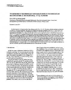
LEAST MEAN SQUARE (LMS) ADAPTIVE TECHNIQUE The standard structure for the adaptive filter is illustrated in Fig. 1. It is actually an adaptive linear combiner (ALC) shown in the form of a transversal filter with filter size L + 1, where the adjustable tap-weights have values at time n denoted by the tap-weight vector w(n) = [w0(n), wl(n),.., wz(n)] r
(1)
The vector of tap-inputs at time n is denoted by x(n) = Ix(n), x(n - 1)... (n - L)] T
(2)
where the superscript T stands for 'transpose'. During the adaptive filtering process, an additional signal d(n), called the desired response, provides a frame 409
410
M. L. Wang, F. Wu noise
(w,, e) = (0, o ~ ) ~ System
~:::,::...
2-~
,c)=
/____J I- o Y~~( )
error,
/
/
w~ adaptive filter
w2-axis
I
Fig. 1. Modeling for FIR (finite impulse response) system.
of reference for adjusting the tap-weights of the filter. The corresponding estimate of the desired filter output is y(n), which can be expressed as y(n) = wT (n)X(n) = xT (n)(n)
(3)
The estimated error due to comparing the actual values of output and the values of the desired response d(n) is given by e(n) = d(n) - y(n)
(4)
The assumptions for the input signal and the desired response state that both input signal and desired response are stationary, and input signal and desired response are correlated with each other and are jointly stationary. Then the mean-squared error function ~(n) at time n is a quadratic function of the tap-weight vector as illustrated below. ~(n) = E[e(n) 2] = Et(d(n ) - wT(n)x(n)) 2]
wl-axls
(5)
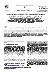
= E[d(n) 2] + 2wr(n)P + w r ( n ) R w ( n ) where E[.] is the expectation operator, and R and P are defined as follows. R = E[x(n)x(n) r] e = E[d(n)x(n) r] Therefore, the square matrix R is the input correlation matrix, and the vector P is the set of cross-correlation between the desired response and the input components. The mean-squared error function ~(n), depending on the tap-weight vector, is a bowl-shaped surface with a unique minimum if n for the tap-weight vector is equal to 2 (Fig. 2). This surface is called the error performance surface of the adaptive filter) It has a single global minimum. The adaptive process causes the tap-weight vector to seek the minimum of the error performance surface using the gradient method, and the minimum point of that surface can be found theoretically by obtaining an expression for the gradient and setting it
Fig. 2. Location of the minimum of the MSE surface.
equal to zero. The result is a weight vector which takes on the optimal Viener solution w*. It is expressed as s w* = R-1P
(6)
the minimum mean-squared error is then given by ~min = E[d(n2)] - Prw*
(7)
In order to find the minimum mean-squared error,
~min, Widrow & Stearns 6 proposed the simple and effective LMS algorithm based on an estimate of the gradient weight vector, V(n), as V(n) = Vw(n)[e(n)2] = Vw(n)[(d(n) - wr(n)x(n)) 2]
(8)
= -2e(n)x(n) where V(n) is the estimated gradient at time n, and Vw(,) is the gradient of e(n) 2 with respect to 2(n). With this simple estimate of the gradient, the LMS form for the steepest descent weight update becomes w(n + 1) = w(n) - #V(n)
(9)
= w(n) + 2#e(n)x(n) where # is a gain constant that regulates the speed and stability of the adaptive algorithm, or it can be expressed as a scalar update form for each weight: wi(n + 1) = wi(n ) + 2p,e(n)x(n - i); 0 < i < L
(10)
The bound on # for convergence of the weight vector mean is derived in the literature by, 6 as 0