proximate models for the fitness evaluation in evolution- ary design optimization.
To improve the quality of the neural network models, structure optimization of ...
Soft Computing (In press) Special Issue on Approximation and Learning in Evolutionary Computation.Guest Edited by Y. Jin et al
Published in: Soft Computing, 9(1), pp. 21-28, 2005
Structure Optimization of Neural Networks for Evolutionary Design Optimization Michael H¨ usken1 , Yaochu Jin2 , and Bernhard Sendhoff2 1 2
Institut f¨ ur Neuroinformatik, Ruhr-Universit¨ at Bochum, 44780 Bochum, Germany Honda Research Institute Europe 63073 Offenbach/Main, Germany
The date of receipt and acceptance will be inserted by the editor
Abstract We study the use of neural networks as approximate models for the fitness evaluation in evolutionary design optimization. To improve the quality of the neural network models, structure optimization of these networks is performed with respect to two different criteria: One is the commonly used approximation error with respect to all available data, and the other is the ability of the networks to learn different problems of a common class of problems fast and with high accuracy. Simulation results from turbine blade optimizations using the structurally optimized neural network models are presented to show that the performance of the models can be improved significantly through structure optimization. Keywords: Design optimization, neural networks, evolutionary algorithms, fitness approximation
1 Introduction In many real-world applications of evolutionary computation, fitness evaluations are highly time-consuming. One attempt to reduce the computation time is to replace the original fitness function, at least in part, by an approximate model with a much lower computational cost [10]. Such models are also known as meta-models or surrogates in optimization. In [9] a framework for evolutionary optimization using approximate models with application to design optimization has been proposed. In this framework, the approximate model is combined with the original fitness function to control the evolutionary process, i.e., to decide how often the approximate model should be used instead of the original fitness function, to ensure the convergence of the evolutionary algorithm to a correct optimum of the original problem and to reduce the computational expense as much as possible. The basic idea is that the higher the quality of the model is, the more often it should substitute the original fitness function. This has been termed as evolution control in [9],
also known as model management in design optimization with approximate models [2]. In many applications fully connected feed-forward neural networks have been used as approximate models, although it is well known that the approximation quality and learning efficiency of neural networks strongly depend on their architecture. The learning capability of the neural networks becomes particularly important when online learning needs to be performed during optimization. In this paper, structural optimization of neural networks is carried out before they are employed for fitness evaluations in evolutionary design optimizations. Since structure optimization based on the approximation error does not explicitly deal with the learning capability of neural networks, a method for learning problem classes suggested in [6] is also investigated. The quality of the neural network models is usually evaluated with the quadratic approximation error. However, the approximation task in the context of a metamodel is not the same as in the context of optimal prediction. For a meta-model a qualitative approximation is often sufficient, whereas prediction needs a minimal quantitative difference. The examples in Figure 1 (a) and (b) clarify what we mean by “qualitative”. The approximation accuracy of the neural networks shown might be quite unsatisfying, but nevertheless, these approximate models are still able to lead an optimization algorithm to the correct minimum of the fitness function. In this sense, the quality of the model as a meta-model is sufficient, although the approximation error is high. Thus, it is worth considering other quality measures to evaluate neural networks that are used as surrogates in design optimization. The remainder of the paper is organized as follows. In Section 2, the framework for model management in design optimization used in this paper is reviewed briefly. Several measures for the model quality are discussed in Section 3. Thereafter, two approaches to structure optimization of neural networks are presented in Sec-
2
Michael H¨ usken, Yaochu Jin, and Bernhard Sendhoff (b) original fitness neural network
fitness φ
fitness φ
(a)
neural network original fitness
i
2 The Framework for Model Management It is not trivial to decide when to use the computationally efficient approximate model instead of the timeconsuming original fitness function during the optimization. There are two basic issues that must be taken into account in applying approximate models in optimization. First, the optimization algorithm should converge to the global optimum of the original fitness function. As the empirical study in [8] indicates, the original fitness function should usually be used in over 50% of the fitness evaluations to guarantee the correct convergence of the evolutionary algorithm. Second, the approximate models should be used as often as possible to reduce the computation time. To this end, a framework for model management in design optimization has been proposed in [9, 10]. The basic idea of the framework is that the higher the model quality, the more often the approximate models should be used. As shown in Figure 2, the evolutionary design optimization process is divided into succeeding control cycles consisting of a sequence of ζ generations. In the figure, individuals evaluated using the original fitness function are denoted by a shaded rectangle, whereas the individuals evaluated using the approximate model are represented by an unfilled rectangle. In the first η generations of the control cycle, the individuals are evaluated using the original fitness function, in the remaining generations, fitness evaluations are performed using the approximate model. The individuals in these η generations are denoted as controlled individuals. During the first η generations, the model output is compared with the original fitness function to evaluate the model quality to adapt the frequency value η. Moreover, the generated data of the original fitness function can be used to train the neural network models during the design optimization.
i+eta
i+xi
i+eta+1
eta
...
Fig. 1 Although the approximation errors of the neural network models are quite large, the optimization by means of the approximate models leads to the desired minimum of the fitness.
tion 4. The optimized networks are applied as approximate models in the design optimization of turbine blades in Section 5, where comparative studies are carried out to show the influence of the different strategies for neural network structure optimization on the design optimization outcome. A brief discussion and the conclusion of the paper is provided in Section 6.
i+1
Model quality estimation
...
Model update
Fig. 2 A framework for model management in evolutionary design optimization. The gray and white boxes indicate individuals that are evaluated by means of the original fitness function or the approximate model, respectively. Each column of boxes indicate one generation.
3 Measures for the Quality of Approximate Models As previously mentioned one of the main issues in the design and use of approximate models is their quality. However, quality is not inevitably equivalent to a close quantitative approximation of the fitness function, but should reflect the purpose in the design of the model, i.e., to ensure the selection of the best individuals in terms of the original fitness function, see Figure 1. In the following, we define different measures based on these considerations. Some of these measures rely on the particular selection scheme of evolution strategies. However, the basic idea can straightforwardly be applied to any kind of evolutionary algorithms. 3.1 Definition of Quality Measures The most popular measure for model quality is the mean squared difference between the individual’s original fitness function φ(orig.) and the output of the approximate model φ(model) �2 1 � � (model) (orig.) φj − φj n j=1 n
E (mse) =
.
(1)
Here, the mean squared difference is averaged over n different individuals taken into account for the estimation of the quality measure, e.g., the n = λ offspring individuals in one generation or the n = η λ controlled individuals in one control cycle. When using (1) during training, additional mechanisms to avoid overfitting should be applied. Generally speaking, a model with good approximation quality ensures the correct evaluation and consequently the correct selection of the individuals. However, from the evolutionary optimization point of view, only the correct selection is of importance. In the following, we define a number of measures that focus primarily on the correct model-based selection and not on the approximation accuracy. The exact definitions of the first two
Structure Optimization of Neural Networks for Evolutionary Design Optimization
measures depend on the selection method. Although we only give expressions for the case of the (µ, λ)-selection with λ ≥ 2µ, which is of particular relevance in our design optimization algorithm, it is in principle possible to extend the ideas and expressions to other selection schemes. The first measure we suggest is based on the number of individuals that have been selected correctly using the approximate model: ρ(sel.) =
ξ − �ξ� µ − �ξ�
,
�ξ� =
µ �
� µ �� λ−µ � m
m=0 2
=
µ λ
m
µ−m
� λ� µ
.
(3)
of ξ in case of random selections is used as a normalization in (2). It can be seen that if all µ parent individuals are selected correctly, the measure reaches its maximum of ρ(sel.) = 1, and that negative values indicate that the selection based on the approximate model is worse than a random selection. The measure ρ(sel.) only evaluates the absolute number of correctly selected individuals. However, in case of ρ(sel.) < 1 the measure does not indicate, whether the (µ + 1)-th or the worst offspring individual has been selected, which may have significant influence on the evolution process. Therefore, the measure ρ(sel.) is extended to include the rank of the selected individuals, calculated based on the original fitness function. A model is assumed to be good, if the rank of the selected individuals based on the approximate model is above-average according to the rank based on the original fitness function. The definition of the extended measure ρ(∼sel.) is as follows: The approximate model gets a grade of λ−m, if the m-th best individual based on the original fitness function is selected. Thus, the quality of the approximate model can be indicated by summing up the grades of the selected individuals, which is denoted by π. It is obvious that π reaches its maximum, if all µ individuals are selected correctly: π
(max.)
=
µ �
as the expectation �π� = random selection: ρ(∼sel.) =
µλ 2
for the case of a purely
π − �π� π (max.) − �π�
.
(5)
Besides these two problem-dependent measures for evaluating the quality of the approximate model, two established measures — the rank correlation and the (continuous) correlation — partially fit the requirements formulated above. The rank correlation [13], given by
(2)
where ξ (0 ≤ ξ ≤ µ) is the number of correctly selected individuals, i.e., the number of individuals that would have also been selected if the original fitness function had been used for fitness evaluation. The expectation
3
ρ
(rank)
�λ 6 l=0 d2l =1− λ(λ2 − 1)
,
(6)
is a measure for the monotonic relation between the ranks of two variables. In our case, dl is the difference between the ranks of the l-th offspring individual based on the original fitness function and on the approximate model. The range of ρ(rank) is the interval [−1; 1]. The higher the value of ρ(rank) , the stronger the monotonic relation with a positive slope between the ranks of the two variables. In contrast to ρ(∼sel.) , the rank correlation does not only take the ranking of the selected individuals, but also the ranks of all individuals into account. This is more than needed for the model-based selection, however, it gives a good estimation of the ability of the model to distinguish between good and bad individuals, which is the basis for a correct model-based selection. Another possibility to quantify the idea that the approximate model should ensure correct selection, but not necessarily reproduce the correct fitness values, is given by the (continuous) correlation between the approximate model and the original fitness function: �n � (model) ¯(model) � � (orig.) ¯(orig.) � 1 −φ −φ φj j=1 φj n ρ(corr.) = σ (modell) σ (orig.) (7) Here, φ¯(model) and φ¯(orig.) are the mean values and σ (modell) and σ (orig.) the standard deviations of the approximate model output and original fitness function, respectively. The properties of the correlation is related to both the rank based measures introduced above and the mean squared error. It is not a measure for the difference between model output and original fitness, but evaluates a monotonic relation between them. In addition, the range of this measure is known and therefore ρ(corr.) is easier to evaluate than E (mse) . Besides, ρ(corr.) is differentiable, which allows to use gradient-based methods for the adaptation of the model.
(λ − m)
m=1
� � µ+1 = µ λ− 2
.
(4)
In analogy to (2) the measure ρ(∼sel.) is defined by transforming π linearly, using the maximum π (max.) as well
4 Evolutionary Optimization of Neural Networks The performance of neural networks does not only depend on the choice of the weights, but also strongly
.
4
Michael H¨ usken, Yaochu Jin, and Bernhard Sendhoff
on the choice of the architecture or structure1 , i.e., the graph describing the number of neurons and the way the neurons are connected. In particular, the task of fast learning or learning with a small amount of data demands a suitable architecture [5]. Evolutionary structure optimization of the neural networks has proven to be a very efficient approach to choosing the architecture as well as the weights, refer to [15] for a survey. In principle, it is possible to embed the structure optimization of the approximate model into the design optimization algorithm. In this work, we perform structure optimization of the neural networks offline, i.e., before the neural networks are employed as meta-models in the design optimization algorithm. The data for this offline optimization stems from previous design optimization runs. Only the weights will be adapted in every single control cycle during the design optimization as outlined in Section 2. Further details about the structure optimization of the neural networks, in particular the incorporation of life-time learning are given in the following.
4.1 Accuracy-Based Structure Optimization We employ a direct encoding scheme for the structure optimization of neural networks, i.e., every connection and the value of every weight of the networks are encoded in the individual’s genome. Taking into account the characteristics of the structure of neural networks, specific mutation operators have been chosen. Single connections and neurons can be inserted or deleted. Weights are mutated by adding normally distributed random numbers. After mutation, τ iterations of gradient-based learning are introduced using iRprop+ [7], an improved version of the Rprop-algorithm [12]. The purpose of the gradient learning is to fine tune the weights based on the mean squared error of the neural network. The modified weights are encoded back into the individual’s genome after learning, following the effective Lamarckian paradigm [14]. Finally, we use EP-tournament-selection based on fitness values representing the mean squared error of the individuals after learning. To avoid overfitting we use early stopping during learning as well as different data sets for learning and for fitness evaluations. A schematic illustration of the Lamarckian mechanism is shown in Figure 3. Note that the architecture aj of the network encoded by the j-th individual does not change during life-time learning, but that the weights do; here wj and w�j denote the weights before and after learning, respectively. The variable P denotes the problem the networks should learn. This kind of optimization searches for neural networks that represent the input-output mapping induced by a given set of data of the problem P with a minimum error, including the ability to generalize towards 1
We will use the terms architecture and structure synonymously throughout the paper.
P (Data)
w’
w NN(a ,w ) 1 1
NN(a ,w ) λ
λ
1
1
Life−time Learning
wλ
wλ ’ Life−time Learning
NN(a , w’ ) 1 1
NN(a ,w ’ ) λ
λ
t := t + 1
Mutation
Selection
Fig. 3 The Lamarckian mechanism for evolutionary structure optimization of neural networks. The variable N N (aj , w j ) stands for an individual encoding a neural network with architecture aj and weight vector w j .
other data stemming from the same problem P. Therefore, the result is one approximation model with one architecture and initial weight configuration for the whole fitness landscape, i.e. for the mapping from the design space into the performance space.
4.2 Structure Optimization for Problem Classes As discussed in Section 1, the learning capability of neural networks can be as important as the pure performance, the approximation error. This is particularly the case when neural networks are learned online based on a small amount of data, like in the design optimization application where the data is taken from single control cycles. Here the neural networks serving as approximate models are trained at the end of each control cycle, as illustrated in Figure 2. It is intuitive, that the optimal models for the data from one control cycle to the next will share some common architectural aspects, since the population of the design optimization algorithm moves slowly compared to the duration of one control cycle. Furthermore, it can be seen that even different design optimization runs share common aspects. In the last section, the different local approximation problems in each single control cycle were treated as one complex problem. The basic idea behind the approach outlined in this section is firstly to regard each single problem as unique and secondly to group these different problems in a problem class. Note that in general the definition of problem classes is difficult; no appropriate metric exists to define a proper notion of relatedness. In our application, we can circumvent an explicit definition by using the implicit one which we gain from the control framework outlined in Section 2. The approximation in each single control cycle is one problem, the group of all problems defines the class. The advantage of keeping
Structure Optimization of Neural Networks for Evolutionary Design Optimization
the problems separate is to give a clear definition to what we mean by the network’s capacity to learn: How good is the network prepared by the structure optimization task to learn new problems from the class. Thus, if the network meets new areas of the fitness landscape, which is very likely to happen during optimization, the structure which reflects the common aspects of the problem class, allows the network to adapt to this new approximation problem fast and based only on few data. This type of generalization has been termed second order generalization in [4] because instead of generalizing between different data sets, the network has to cope with varying problems. In [4], the authors investigate different structure optimization approaches in order to integrate common aspects of the problem class in the network’s structure such that the network is well prepared for learning the different particular problems, i.e. the models in different control cycles. We extend and apply these methods to the domain of approximate modeling. Assume that data from ν control cycles are available for offline structure optimization of the neural networks. Instead of learning the whole problem P during life-time in one generation of the structure optimization, the problem is divided into ν subproblems P1 , P2 , . . . , Pν according to the ν evolution control cycles. During the life-time learning of the j-th individual (1 ≤ j ≤ λ) the network represented by this individual is first trained on the data of the problem P1 for τ iterations, resulting in the weight vector wj,1 and the approximate error Ej,1 . Thereafter, this network with weight configuration wj,1 is further trained on the problem P2 , resulting in the weight vector wj,2 and the approximation error Ej,2 . This process continues until the j-th network has been trained on all ν problems. A schematic illustration of the algorithm is shown in Figure 4. P1 NN (a , w ) 1
1
w1
NN 1
P2 w 1,1
NN 2
5
ber of different problems, some kind of average weights have to be coded back [6]. Since in the next generation these weights will be the starting configuration in the first control cycle, the influence of the learned weights w j,i should decline with increasing index i of the control cycle: w�j =
ν 1 − γ � i−1 γ w j,i 1 − γ ν i=1
;
0