Design of Neural Networks Claudio Moraga and
European Centre for Soft Computing, 33600 Mieres, Asturias, Spain Dept. Computer Science, University of Dortmund, 44221 Dortmund, Germany
[email protected]
Abstract. The paper offers a critical analysis of the procedure observed in many applications of neural networks. Given a problem to be solved, a favorite NN-architecture is chosen and its parameters tuned with some standard training algorithm, but without taking in consideration relevant features of the problem or possibly its interdisciplinary nature. Three relevant benchmark problems are discussed to illustrate the thesis that “brute force solving is not the same as understanding”. Keywords. Neural networks, pre-processing, problem-oriented design
1. Introduction Since the publication of “the” book of Rumelhart, and McClelland [22] the interest for developing and using neural networks for classification, approximation, and prediction tasks has grown quite impressively. Most nets applied for these tasks are feedforward nets with sigmoidal activation functions and tuned with some improved version (e.g. [13]) of the original gradient descend algorithm for which the name “Backpropagation” was coined, or are RFB-nets, which use non-monotonic activation functions, mostly Gaussian “bells”. It is not quite clear whether the convincing power of the theorems on universal approximation of feedforward neural networks [9], [12] and RBF nets [11] or the effectivity of the training algorithms and the high speed of present PCs, which have contributed to favor a situation in which the “design” of a neural network reduces mainly to finding either per trial and error, or in the best case, by means of an evolutionary algorithm, the optimal number of hidden neurons. This is considered to be a negative trend. This paper analyses three benchmarks to show the results that may be obtained if instead of a “blind approach”, knowledge –(possibly interdisciplinary)- of the designer, related to the problem domain and to fundamentals of neural networks, is taken into consideration and becomes an important component of the design process. The selected benchmark problems are: The two spirals, the n-bit parity and the RESEX time series problems. The two spirals problem was posed by Alexis Wieland [26] in the late 80s as a challenge to the “triumphalists” in the NN-community. Two sets of 97 points each, are distributed along two concentric spirals. See Fig. 1. A neural network should be obtained, able to separate the two classes. Later on the problem was made tougher, by asking the neural network to separate the spirals and
not only the sample points, i.e. the neural network was required to exhibit a very good generalization. Soon after the statement of the problem appeared the first solutions by Lang and Witbrock [14] and by Fahlman and Lebière [8]. Even though both solutions represented totally different architectures, both used 15 hidden neurons. Today, the two spirals problem is a typical homework in any neural networks course and probably most students solve the problem using the method criticized in the former paragraph. A 2-30-1 solution of recent times may be found in [17]. The second selected problem is the n-bit parity problem. A neural network with n binary inputs should be able to distinguish when the number of 1s in the input is even or odd and, following [24] it is possible to build such a neural networks with sigmoidal activation function using at most n/2 +1 hidden neurons if n is even or (n+1)/2, if n is odd. If shortcut connections are allowed, then a solution with only n/2 hidden neurons if n is even is possible [18]. A few solutions matching the bounds stated above may be found in the scientific literature. A solution without shortcuts and using only n/2 hidden neurons for the 8-bit parity problem is given in [2]. The RESEX time series [16] is based on the calling activity of the clients of a Canadian telephone company and is famous for a big outlier due to a special low-cost calling offer on Christmas time. This makes of this series a very tough prediction problem (not only) for a neural network.
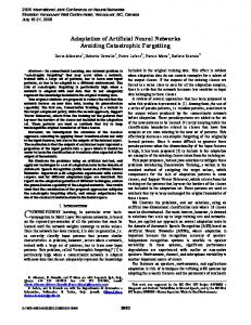
2. From the problem to the neural network The two spirals problem, as stated, is indeed a difficult problem for a feedforward neural network using sigmoidal activation functions. However, experiences from signal processing, for instance, have shown that depending on the problem, it may be better to process the signal in the time domain or in the frequency domain. A rather obvious first choice for a different representation of the two spirals problem is to use polar coordinates. Every point with original coordinates (x, y) will be given the new coordinates (ρ, θ), where ρ = (x2 + y2)1/2 and θ = arctan(y/x) + π·sign(y). The computational complexity of these operations is relatively low and could be assigned as transfer functions of two auxiliary neurons with x and y as inputs. Using a new orthogonal coordinates system (ρ, θ), the representation of the problem in the new domain is illustrated at the right hand side of Fig. 1. The fact that the two spirals look now as a set of regularly alternating straight line segments within the [-π, π] interval (each segment corresponding to a different class than that of its neighbor segments), is a consequence of the fact that A. Wieland must have chosen Archimedean spirals when he designed the problem. This kind of spirals has the property that the radius grows linearly with respect to the angle. From Fig. 1 (right) it may be seen that the slope of the line segments is 1/π and that, if θ = 0, a symmetric square wave of period T = 2 could separate the alternating line segments corresponding to different classes (see Fig. 2). A symmetric square wave may be expressed as sign(sine(ωρ)), where ω denotes the angular frequency. The period T of a periodic function satisfies the condition ωT =2π, from where ω = 2π/T = 2π/2 = π. Therefore the required square wave is s = sign(sine(πρ)). If θ ≠ 0 a proper lag is required, which is proportional to the product of the value of θ and the slope of the line segment. Finally, the square
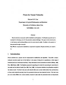
wave accomplishing the separation of the two classes is given by s = sign(sine(πρ – θ/π)). This analysis leads to a neural network consisting of three neurons: the two auxiliary neurons mentioned above and a third one having as inputs ρ and θ, and as activation function, the periodic symmetric square wave s. All weights are equal to 1 and all biases are equal to 0. Furthermore, no training is needed. See Fig. 2. It may be argued that the proposed system is not really a neural network, however it satisfies the definition of a neural network: it is a distributed dedicated computing system, each neuron computes a single function of bounded complexity without requiring memory and the interconnection structure is as dense as possible by three neurons under the feedforward without shortcuts model.
Fig. 1. The two spirals problem: left: representation in Cartesian coordinates. Right: representation in polar coordinates. (Vertical axis: radius ρ; horizontal axis, angle θ in radians)
s ρ
θ
ρ
0 θ x
α
y
Fig. 2. Left: A minimal neural network designed to efficiently solve the two spirals problem. Right: Pseudo perspective of a partial view of the separation of the two unrolled spirals, where tan(α) = 1/π
Solving the two spirals problem using polar coordinates was preliminary discussed in [19], but leading to a more complex solution, even though also without requiring learning the weights. The idea was later on also considered in [3], providing still a different final solution, however with emphasis in training the weights. As mentioned in the introduction, important efforts and contributions have been done related to the n-bit parity problem. Most of them have focused on working with
feedforward nets, eventually with shortcuts, using sigmoidal activation functions. An alternative approach was presented in [25] by introducing an “unusual” activation function quite different from a sigmoide to solve the parity problem with only two hidden neurons. In [15] the authors discuss the use of “product units” [7] instead of sigmoidal or Gaussian neurons. In these units, exponents are associated to the input variables. The output of the unit is the product of the exponentially weighted inputs. Obviously product units cannot directly process Boolean signals and the recoding to the set {1, -1} is a needed preprocessing. It becomes apparent that if the weights are chosen to be odd, a single product unit followed by proper decoding solves the parity problem. In [15] however the authors were interested in using the parity problem to test the ability of different training algorithms to “learn” appropriate weights. Unfortunately, these lines of research do not seem to have been continued. In what follows it is shown that is possible to design a problem-oriented activation function to solve the problem with only one neuron accepting the standard weighted sum of inputs, without needing a recoding of the inputs and decoding of the output and without training of the weights. Let A(x) denote the weighted sum of the inputs to a neuron. The standard sigmoidal activation function is given by f(x) = [1 + exp(-A(x))]-1. A parameterized extension was introduced in [10] as f(x) = a[1 + exp(-bA(x))]-1 + c, where the parameters a,b and c were also adjusted to minimize the square error of performance. Notice that if a = 1 and c = 0, then f(x) behaves as the classical sigmoide, except that the parameter b contributes to increase the speed of convergence by modifying all weights of a given neuron at the same time. If on the other hand, a = 2 and c = -1, then f(x) behaves like a hyperbolic tangent function. A different view may be obtained by using k –A(x) instead of exp(-b(A(x)) and by adjusting k instead of b. This leads to f(x) = a[1 + k.-A(x)]-1. Notice that by choosing a = ½ , k = -1, setting all weights to 1 and not taking the inverse value of the expression, the activation function turns to: f(x) = ½ [1 + (-1) –A(x)] –A(x)
(1)
It is simple to see that whenever A(x) is even, (-1) = 1 and f(x) = 1; meanwhile if A(x) is odd, then (-1) –A(x) = -1 and f(x) = 0. This means that a single neuron with this activation function, setting all weights to 1 and all biases to 0, is all that is needed to solve the n-parity problem for any n and, by the way, without training and without requiring the domain and codomain of the parity function to be {-1, 1}. It may be argued, that a single neuron is not a net. If this objection is accepted, the above results proves that no neural network is needed to solve the n-parity problem, but only a neuron designed to accomplish parallel counting modulo 2 and adding 1. The proposed solution was obtained by adapting a classical activation function to the requirements of the problem. It is however very closely related to the single neuron solution to the n-bit parity problem, presented in [1]. This other solution is formally based on principles of multiple-valued threshold logic over the field of complex numbers. The method requires using complex-valued weights, but up to n = 5 all binary functions may be realized with a single neuron. The effectiveness of the training algorithms for neural networks and the similarities between neural networks and auto regressive systems (see e.g. [4]) possibly motivated the interest in using neural networks for prediction in the context
of time series. The first intuitive approach to apply a neural network to predict one next event of a time series is to use the past history of the series to train a neural network using a sliding “time window”. The samples within the window are the inputs to the neural network and the output is the predicted next event. Since during the training phase the next event is known, a prediction error may be calculated, which should be minimized by adjusting the weights of the network. The window moves one time step ahead and the process is repeated. This continues until all past samples are processed and the final prediction error is within tolerances. It is easy to see that the width of the time window is one additional parameter that should be adjusted. When the last block of samples is processed, the first actual prediction takes place. If the time window is moved one further step ahead, the just predicted signal will be within the time window, i.e., feedback is needed at the start of the prediction phase. (See Fig. 3, left). The above discussed scheme works particularly well in the case of short-term predictions (see e.g. [6]), since nonstationarity or seasonality of the time series may possibly be not noticeable. More sophisticated training algorithms have allowed however to use the above scheme together with support vector machines, even with chaotic series [21]. Time series analysis is however a well established research area in Statistics, starting at least in 1976 with the publication of the seminal book of Box and Jenkins [5]. Statisticians have developed sound methods not only to find the appropriate width of the time window, but also to evaluate the relevance of the data within the window. Non relevant data within the time window adds a noise-like effect increasing the difficulty of the predicting process. The RESEX time series is based on measurements of the internal connections of residential telephone extensions in a certain area of Canada during a period of 89 months [16]. The series is characterized by a clear yearly seasonality and a big outlier –(atypical value)- near the end of the series, corresponding to a low price Christmas promotion of the telephone company (see Fig. 4, left). Box and Jenkins [5] introduced a seasonal ARIMA model –(AutoRegressive model with Integrated Moving Average)- which, for this series, corresponds to ARIMA(2,0,0)(0,1,0)12. From this model it is possible to deduce that the relevant lags are { -1, -2, -12, -13, -14}. With this information, a one neuron net with sigmoidal activation function was able to predict the behaviour of the series on a one step basis [23]. See Fig. 4 (right hand side). 3. Conclusions The discussed design of neural networks for three benchmark problems has shown that by including (eventually interdisciplinary) knowledge about the problem and about fundamentals of neural networks, both effectiveness and efficiency of the solution may be increased. Taking advantage of the methods developed long ago by statisticians it was possible to obtain a minimal solution to the prediction problem without facing an online noise filtering problem. The solution for the two spirals problem exhibits perfect generalization and unconstrained scalability: should the spirals be prolonged another round, then the same neural net would solve the problem. Similarly, the neuron designed to solve the parity problem, solves the problem for any
n. Both the solution for the two spirals problem and the parity problem were obtained without training: the value of the free parameters could be deduced or calculated. This means that in this case, by trying to do a “knowledge-based design” of a neural network, an analytical solution of the problem was obtained. The strategies discussed above are not new, but have often been absent when applying neural networks to solve a problem, with possibly the exception of Kernelbased methods (see e.g. [20]), which use idea of change of domain, as a basic component of their design strategy. A nonlinear problem is mapped into a linear domain, where a solution is most of the time simple, to later translate back the solution to the original domain. People in pattern recognition are used to do first feature extraction, which is a search for relevant data, before starting to do classification. Statisticians can do that formally in the case of time series prediction. It is not unusual that engineers solve differential equations applying the Laplace transform. The “pocket calculator” of my generation was the slide-rule, where products and divisions were very efficiently done by adding and subtracting logarithms graphically represented on the rule! Brute force should always be the very last resource. “Brute force solving a problem is not the same as understanding the problem”. Training
Predicting resext-1 resext-2 st
resext-12 resext-13 resext-14
resext
: One time step delay Fig. 3. Left: Time series prediction with a neural network (without taking in account data relevance). Right: An ARIMA-based one-neuron-net to predict the RESEX series
RESEX NN
Fig. 4. Left: The RESEX time series. Right: A neural network based one step prediction
References 1. Aizenberg I.: Solving the parity n problem and other nonlinearly separable problems using a single universal binary neuron. Computational Intelligence. Theory and Applications, (B., Reusch Ed.). Springer Verlag, Berlin, 2006 2. Aizenberg I., Moraga C.: Multilayer feedforward neural network based on multi-valued neurons (MLMVN) and a backpropagation learning algorithm. Soft Computing 11 (2), 169183, 2007 3. Alvarez-Sánchez J.R.: Injecting knowledge into the solution of the two-spiral problem. Neural Computing and Applications 8, 265-272, 1999 4. Allende H., Moraga C., Salas R.: Artificial neural networks in forecasting: A comparative analysis. Kybernetika 38 (6), 685-707, 2002 5. Box G.E., Jenkins G.M.: Time series analysis: forecasting and control. Holden-Day, Oakland CA, USA, 1976 6. Chow T.W.S., Leung C.T.: Nonlinear autoregressive integrated neural network model for short-term load forecasting. IEE Proc. Gener. Transm. Distrib. 143 (5), 500-506, 1996 7. Durbin R., Rumelhart D.: Product units: A computationally powerful and biologically plausible extension to backpropagation networks. Neural Computation 1, 133-142, 1989 8. Fahlman S.E., Lebiere C.: The Cascade Correlation Learning Architecture. In Advances in Neural Information Processing Systems (S. Touretzky, Ed.), Morgan Kaufmann, 1990 9. Funahashi K.I.: On the approximate realization of continuous mappings by neural networks. Neural Networks 2 (3), 183-192, 1989 10. Han J., Moraga C.: The Influence of the Sigmoid Function Parameters on the Speed of Backpropagation Learning. In From Natural to Artificial Neural Computation (J. Mira, Ed.). LNCS 930, 195-201, 1995 11. Hartman E.J., Keeler J.D., Kowalski. J.M.: Layered neural networks with Gaussian hidden units as universal approximators. Neural Computation, 2, 210–215, 1990 12. Hornik K., Stinchcombe M., White H.: Multilayer feedforward neural networks are universal approximators. Neural Networks 2 (5), 359-366, 1989 13. Igel Ch., Huesken M.: Improving the Rprop Learning Algorithm. Proc. 2nd Int. Symposium on Neural Computation. 115-121. Academic Press, 2000 14. Lang K.J., Witbrock M.J.: Learning to tell two spirals apart, Proceedings of the 1988 Connectionist Models Summer School, Morgan Kaufmann, 1988 15. Leerink L.R., Giles C.L., Horne B.G., Marwan A.J.: Learning with product units. Advances in Neural Information Processing, NIPS-94, 537-544, 1994 16. Martin R.D., Smarov A., Vandaele W.: Robust methods for ARIMA models. Proc. Conf. applied time series analysis of economic data, 153-169. (A. Zellner, Ed.), ASA-CensusNBER, 1983 17. Mizutani E., Dreyfus S.E.: MLP’s hidden-node saturations and insensitivity to initial weights in two classification benchmark problems: parity and two spirals. Proc. IEEE Intl. Joint Conf. on Neural Networks, 2831-2836. IEEE-CS-Press, 2002 18. Minor J.M.: Parity with two layer feedforward net. Neural Networks 6, 705-707, 1993 19. Moraga C., Han J.: Problem Solving =/= Problem understanding. Proceedings XVI International Conference of the Chilean Computer Science Society, 22–30. SCCC–Press, Santiago, 1996 20. Müller K.-R., Mika S., Rätsch G., Tsuda K., Schölkopf B.: An introduction to Kernel-based learning algorithms. Chapter 4 of Handbook of Neural Networks Signal Processing (Yu Hen Hu, Yenq-Neng Hwang, Eds.), CRC-Press, 2002 21. Müller K.-R., Smola A., Rätsch G., Schölkopf B., Kohlmorgen J., Vapnik V.: Using Support Vector Machines for Time Series Prediction. Proc. of the Int. Conf. on Artificial Neural Networks ICANN ‘97. (W. Gerstner, A. Germond, M. Hasler, J.-D. Nicoud, Eds.), LNCS 1327, 999-1004, Springer Berlin, 1997
22. Rumelhart D.E., McClelland J.L.: Parallel Distributed Processing: Explorations in the Microstructure of Cognition. The MIT Press, 1986 23. Salas R.: Private communication, 2002 and 2007 24. Sontag E.D.: Feedforward nets for interpolation and classification. Jr. Comput. Systems Science 45, 20-48, 1992 25. Stork D.G., Allen J.D.: How to solve the N-bit parity problem with two hidden units. Neural Networks 5, 923-926, 1992 26. Wieland A.: Two spirals. CMU Repository of Neural Network Benchmarks, 1988. http://www.bolz.cs.cmu.edu/benchmarks/two-spirals.html