Available online at www.sciencedirect.com
ScienceDirect Procedia Computer Science 48 (2015) 802 – 808
International Conference on Intelligent Computing, Communication & Convergence (ICCC-2014) (ICCC-2015) Conference Organized by Interscience Institute of Management and Technology, Bhubaneswar, Odisha, India
Neuro Structure Optimization Using Adaptive Particle Swarm Optimization Sushanta Kumar Panigrahia, Amaresh Sahub, Sabyasachi Pattnaikc * a
Interscience Institute of Management & Technology, Bhubaneswar, Odisha, India b Siksha ‘O’ Anusandhan University, Bhubaneswar, Odisha, India c Fakir Mohan University, Balasore, Odisha, India
Abstract In this paper a method to optimize the structure of neural network named as Adaptive Particle Swarm Optimization (PSO) has been proposed. In this method nested PSO has been used. Each particle in outer PSO is used for different network construction. The particles update themselves in each iteration by following the global best and personal best performances. The inner PSO is used for training the networks and evaluate the performance of the networks. The effectiveness of this method is tested on many benchmark datasets to find out their optimum structure and the results are compared with other population based methods and finally it is implemented on classification using neural network in data mining. © 2015 The Authors. Published by Elsevier B.V. This is an open access article under the CC BY-NC-ND license (http://creativecommons.org/licenses/by-nc-nd/4.0/). Peer-review under responsibility of scientific committee of International Conference on Computer, Communication and Convergence (ICCC 2015) Keywords:Artificial neuralnNetwork; particle swarm optimization; teaching learning based optimization.
1. Introduction Increasing productivity, decreasing costs, and maintaining high product quality at the same time are the main challenges of industries today. The proper selection of machining parameters is an important step towards meeting these goals and thus gaining a competitive advantage. Several researchers have attempted to design and meet these
* Corresponding author. Tel.: 91-9861261763 E-mail address:
[email protected]
1877-0509 © 2015 The Authors. Published by Elsevier B.V. This is an open access article under the CC BY-NC-ND license (http://creativecommons.org/licenses/by-nc-nd/4.0/). Peer-review under responsibility of scientific committee of International Conference on Computer, Communication and Convergence (ICCC 2015) doi:10.1016/j.procs.2015.04.218
Sushanta Kumar Panigrahi et al. / Procedia Computer Science 48 (2015) 802 – 808
803
goals. Artificial Neural Network (ANN) is the best option. ANN is an information processing paradigm that is inspired by the way biological neural network or nervous systems process information, such as brain. The processing power of ANN allows the network to learn and adapt. Time to time, the application of Artificial Neural Network (ANN) in industries has been accepted very rapidly. In the growing interest of using ANN is to assist building model structure with particular characteristics such as the ability to learn or adapt, to organize or to generalize data. Up-to-date designing optimal network architecture is made by a human expert and requires a tedious trial and error process. Especially automatic determination of the optimal number of hidden layers and nodes in each hidden layer is the most critical task [1, 2, 3]. Computational models using ANN are dependent on the network structure (topology, connections, neurons number) and their operational parameters (learning rate, momentum, etc). In other words, the form in which the network architecture is defined affects significantly its performance that can be classified in learning speed, generalization capacity, fault tolerance and accuracy in the learning. It is hard to project an efficient Neural Network (NN), even there are some techniques those come empirical knowledge, which is not always get right. This happens due to inherent particularities to the physical processes in which the networks are applied [1, 2, 3, 4, 5, 6, 7]. In this paper evolutionary system, such as Adaptive Particle Swarm Optimization (APSO) is used for the training and the network for better generalization performances and low training errors. 2. Evolutionary system Evolutionary System is a research area of Computer Science, which draws inspiration from the process of natural evolution. Evolutionary computation, offers practical advantages to the researcher facing difficult optimization problems. These advantages are multifold, including the simplicity of the approach, its robust response in changing circumstance, its flexibility and many other facets. The evolutionary approach can be applied to problems where heuristic solutions are not available or generally lead to unsatisfactory results. Thus evolutionary computing is needed for Developing automated problem solvers, where the most powerful natural problem solvers are human Brain and evolutionary process. In this work evolutionary system such as adaptive PSO is used to design architecture of ANN and is used for low training errors of ANN’s as well as to find the appropriate network architecture [5, 6, 7]. 2.1. Adaptive PSO Dr. Russell Eberhart and Dr.James Kennedy first introduced particle Swarm Optimization in 1995. As described by Eberhart and Kennedy, the PSO algorithm is an adaptive algorithm based on a social-psychological metaphor; a population of individuals (referred to as particles) adapts by returning stochastically toward previously successful regions. In PSO algorithm, supposed in D dimensions search space, a particle swarm have m particles. The position of swarm i is xi = ( xi1, xi2, xi3, …, xiD ,) , i =1,2, ….,m . The best position of i is individual historical best position Pi, and the best fitness is individual historical best fitness of i. Vi is flight velocity of the swarm i. The best position of the particle swarm is the position of global best particle and the best fitness of the swarm is the fitness of global best particle. In general, the update formulas of particle i are as follows: νn+1id = χ(ωνnid + c1r1(pnid – xnid) + c2r2(pngd – xnid)) n+1
x
id
=x
n
id
n+1
+ν
id
(1) (2)
In the formulas: χ is contracting factor, ω is inertia weight, c1 and c2 are acceleration factors; r1 and r2 are both random numbers in [0, 1] [8, 9, 10, 11, 12]. As evolution goes on, the swarm might undergo an undesired process of diversity loss. Some particles become inactively while lost both of the global and local search capability in the next generations. For a particle, the lost of global search capability means that it will be only flying within a quite small space, which will be occurs when its location and pbest is close to gbest (if the gbest has not significant change) and its velocity is close to zero (for all dimensions) according to the equation (1); the lost of local search capability means that the possible flying cannot
804
Sushanta Kumar Panigrahi et al. / Procedia Computer Science 48 (2015) 802 – 808
lead perceptible effect on its fitness. From the theory of self-organization, if the system is going to be in equilibrium, the evolution process will be stagnated. If gbest is located in a local optimum, then the premature convergence occurring as all the particles become inactively. To stimulate the swarm with sustainable development, the inactive particle should be replaced by a fresh one adaptively so as to keep the non-linear relations of feedback in equation (1) efficiently by maintaining the social diversity of swarm. This is known as adaptive particle swarm optimization (APSO) [13, 14, 15, 16, 17, 18, 19, 20]. However, it is hard to identify the inactive particles, since the local search capability of a particle is highly dependent on the specific location in the complex fitness landscape for different problems. Based on these facts, we adopt the adaptive particle swarm optimization (APSO) to obtain the optimal solution. 3. Structure optimization through adaptive PSO The performance of neural networks does not depend only on the choice of the weights, but also strongly on the structure, i.e., the number of neurons and the way the neurons are connected. In particular, the task of fast learning or learning with a small amount of data demands a suitable architecture. Evolutionary structure optimization of the neural networks has proven to be a very efficient approach in choosing the structure as well as the weights. In principle, it is possible to embed the structure optimization of the approximate model into the design optimization algorithm. In this work, 8×8 random matrix of populations had been taken for structure optimization for data set Wine, similarly, for Iris, Pima and Bupa. Each column in the matrix represents the structure of intermediate layer of the neural network. Where initial and final layers were fix according to input size of datasets. So, there are 8 different particles networks are considered for finding out the optimum structure for a dataset. In the proposed method PSO is nested in Inner and outer loop. The outer loop is used to optimize the structure of neural networks and inner loop is used to find out the training error values of applied structures. In the outer layer the particle which gives the minimum mean square error value is considered as global best and all particles have their respective personal best mean square error values. In each iteration particles adjusted their structures by following the global best particle and their personal best structures. Particles structures are trained again in inner loop by using PSO. Minimum 2 nodes and maximum 9 nodes in intermediate layer of each network 3.1. Structure optimization algorithm through adaptive PSO for M x N matrix Input the dataset Initialize the percentage of training and testing data Separate the training and testing data Initialize the Weights, Velocities and Control parameters and the maximum number of time the function evaluation through PSO (i.e Maxiter) Initialize the population of M×N matrix with random values between 0 and 9(maximum 9 nodes and minimum 0 nodes in a layer) Where, M represents the number hidden layers and N represents the number of particle in Population Find out the integer matrix for training Calculate the fitness values of N numbers of Particles by applying PSO training algorithm. Find the particle giving the best fitness value/Minimum training error. Convert the particles values to fractional values by dividing each by 10 Initialize the velocities of all elements in the population For loop 1 to Maxiter Calculate position of the particle giving best fitness value from population For iteration from 1 to number of particles Calculate the global best value of all particles Update the weight for each Iteration Calculate the velocities for all particles Update the velocities of each particle in the range of Maximum velocity and Minimum velocity Update the elements of the particles by using velocities
Sushanta Kumar Panigrahi et al. / Procedia Computer Science 48 (2015) 802 – 808
Update the values of particles in the range 0.9 and 0.2 Calculate the fitness values of all particles End of iteration Update the personal best values of each particle Update the global best from fitness value of all particles End of for loop Train the best network by using PSO and MTLBO by using best particle from population to calculate error and accuracy in training and testing sets. 3.2. Experimental setup for adaptive PSO In the Proposed method first the 8×8 random matrix is generated and the values are lying between 0.2 and 0.9, because in the intermediate layers of the network structure can hold minimum 2 nodes and maximum 9 nodes in our assumption. Therefore, the 8×8 random matrix was multiplied by 10 and then converted to integer values for network training. For optimizing the neural network outer PSO worked on fractional matrix and for training, the inner PSO worked on converted integer matrix. If we would consider more than 9 nodes (i.e greater than or equal to 10) in a intermediate layer of the network structure we would consider the random 8×8 marix values between 0.02 and 0.99 means minimum number of nodes 2 and maximum 99 in intermediate layer. This could be found out by multiplying the random matrix by 100 and converting to integer values for training. Similarly for more than 99 nodes in intermediate layer random matrix values would be between 0.002 and 0.999 and training matrix would be found out by multiplying with 1000 and so on. Table-1 represents the random matrix before training and Table-2 shows corresponding integer matrix for training and error finding. Table 1.Random values for optimization (8x8). 0.2325
0.4000
0.7000
0.2000
0.2000
0.7000
0.6000
0.6000
0.4299
0.7000
0.7000
0.4000
0.7000
0.6000
0.5000
0.2000
0
0.4000
0.6000
0.7000
0.3000
0.3000
0.6000
0.5000
0.7843
0.8000
0.7000
0.2000
0.3000
0.3000
0.8000
0.9000
0.2729
0.3000
0.7000
0.3000
0.3000
0.6000
0.4000
0.7000
0.6128
0.6000
0.7000
0.4000
0.7000
0.9000
0.8000
0.3000
0.8213
0.5000
0.7000
0.6000
0.8000
0.5000
0.3000
0.3000
0.6197
0.3000
0.5000
0.6000
0.4000
0.6000
0.5000
0.3000
Table 2.Corresponding structurefor training (8x8). 2
4
7
2
2
7
6
6
4
7
7
4
7
6
5
2
0
4
6
7
3
3
6
5
7
8
7
2
3
3
8
9
2
3
7
3
3
6
4
7
6
6
7
4
7
9
8
3
8
5
7
6
8
5
3
3
6
3
5
6
4
6
5
3
4. Experimental studies The performance of the proposed model is evaluated using the four-benchmark databases taken from the UCI machine repository [21]. Out of these, the most frequently used in the area of neural networks and of neuro-fuzzy
805
806
Sushanta Kumar Panigrahi et al. / Procedia Computer Science 48 (2015) 802 – 808
systems are IRIS, WINE, PIMA and BUPA Liver Disorders datasets. In addition, we have compared the results of MTLBO with other competing classification methods using the aforesaid datasets. 4.1. Description about dataset Let us briefly discuss the datasets, which we have taken for our experimental setup. IRIS: A classification data set based on characteristics of a plant species (length and thickness of its petal and sepal) divided into three distinct classes (Iris Setosa, Iris Versicolor and Iris Virginica). WINE: Data set resulting from chemical analyses performed on three types of wine produced in Italy from grapevines cultivated by different owners in one specific region. PIMA Indians diabetes: Data set related to the diagnosis of diabetes in an Indian population that lives near the city of Phoenix, Arizona. BUPA liver disorders: Data set related to the diagnosis of liver disorders and created by BUPA Medical Research, Ltd. Table 3 presents a summary of the main features of each database that has been used in this study. Table 3.Details of database employed. Dataset
Pattern
Attribute
Class
Patterns in Class1
Class2
Class3
IRIS
150
4
3
50
50
50
WINE
178
13
3
71
59
48
PIMA
768
8
2
500
268
-
BUPA
345
6
2
145
200
-
The results of proposed algorithm to find out structures for various data set is given below, Table 4.Details of database employed. Dataset
Generated intermediate structure
IRIS
9
WINE
9
4
PIMA
9
8
9
BUPA
9
9
9
3
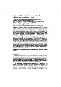
4.2. Result comparison The results obtained for the Iris Dataset, Wine Dataset, Pima Indians Dataset and Bupa Liver Disorders Dataset were compared with the results described in [23] [24] where the performance of several models is presented: NN (nearest neighbor), KNN (k- nearest neighbor, FSS (nearest neighbor with forward sequential selection of feature) and BSS (nearest neighbor with backward sequential selection of feature). MFS (multiple feature subsets), CART (CART decision tree), C4.5 (C4.5 decision tree), FID3.1 (FID3.1 decision tree), MLP (multilayer perceptron) and NEFCLASS. FLANN (functional link artificial neural), simulated annealing (SA) [22], Simple genetic algorithms (SGA) [24], Particle Swarm Optimization (PSONN) [25] and MTLBO [26] using proposed structures for various data sets. The training graphs of PSONN and MTLBONN are given after applying Proposed Structure are given for 100 iterations using different datasets are given below as fig 1. The results in graph showing the comparison of different methods on different datasets
Sushanta Kumar Panigrahi et al. / Procedia Computer Science 48 (2015) 802 – 808
Fig. 1. (a) IRIS; (b) Liver (c) Pima; (d) Wine. Table 5.Comparison results on average performance. Methods
Dataset average performance (in%) Iris
Wine
Pima
Bupa
NN
---
95.2
65.1
60.4
KNN
---
96.7
69.7
61.3
FSS
---
92.8
73.6
56.8
BSS
---
94.8
67.7
60.0
MFS1
---
97.6
68.5
65.4
MFS2
---
97.9
72.5
64.4
C4.5
94.0
---
74.7
---
FID3.1
96.4
---
75.9
---
MLP
---
---
75.2
---
NEF Class
96.0
---
---
---
HNFB
98.67
98.31
77.08
74.49
HNFB1
98.67
99.44
78.26
73.33
Fixed HNFB
98.67
97.8
78.6
---
Adaptive HNFQ
98.67
98.88
77.08
75.07
FLANN
98.67
95.51
78.13
76.23
SGANN
92.93
94.15
74.84
---
MTLBONN
98.87
98.99
79.76
76.25
PSONN
98.86
99.64
---
---
807
808
Sushanta Kumar Panigrahi et al. / Procedia Computer Science 48 (2015) 802 – 808
5. Conclusion In this paper, the performance of the proposed Adaptive PSO method has been used to find out the optimum structure of the Neural Network which is a NP hard and relatively complex problem. Method had been applied on various data sets like Wine, Iris, Pima and Bupa. The results have shown that, these structures can helps to train the networks fastly with minimum training errors. The main disadvantages of proposed method was error existing at the conversion of random values table to integer table during training and more than 10 intermediate nodes may provide better results References 1. C. Zhang, H. Shao. "An ANN’s Evolved by a New Evolutionary System and Its Application" in In Proceedings of the 39th IEEE Conference on Decision and Control, vol. 4, pp. 3562-3563, 2000. 2. E. Eiben and J. E. Smith, Introduction to Evolutionary Computing. Natural Computing Series. MIT Press. Springer. Berlin. (2003). 3. L. Prechelt "Proben1 - A set of neural network benchmark problems and benchmark rules", Technical Report 21/94, Fakultät für Informatik, Universität Karlsruhe, Germany, September, 1994. 4. X. Yao, "Evolving artificil neural networks", Proceedings of the IEEE, vol. 87, pp. 1423-1447, 1999. 5. X. Yao and Y. Liu, "A new evolutionary system for evolving artificial neural networks", IEEE Transactions on Neural Networks, vol. 8, pp. 694-713, 1997. 6. X. Yao, A review of evolutionary artificial neural networks, Int. J. Intell. Syst., 8(4) (1993) 539–567. 7. P.J. Angeline, G.M. Sauders, J.B. Pollack, An evolutionary algorithm that constructs recurrent neural networks, IEEE Trans. Neural Networks 5 (1) (1994) 54–65. 8. J. Kennedy and R. C. Eberhart, “A discrete binary version of the particle swarm algorithm,” in Proc. Conf. Syst., Man Cybern., Piscataway, NJ, 1997, pp. 4104–4108. 9. Kennedy, J., & Eberhart, R. (1995). Particle swarm optimization. In Proc. of IEEE int. conf. on neural networks. vol. 4 (pp. 1942_1948). 10. Y. Shi, R.C. Eberhart, Empirical study of Particle Swarm Optimization, in: Proc. of IEEE World Conference on Evolutionary Computation (1999) 6–9. 11. R. C. Eberhart and Y. Shi, “Comparing inertia weights and constriction factors in particle swarm optimization,” in Proc. Congr. Evolut.Comput., 2000, vol. 1, pp. 84–88. 12. M. Clerc and J. Kennedy, “The particle swarm-explosion, stability, and convergence in a multidimensional complex space,” IEEE Trans.Evolut. Comput., vol. 6, no. 1, pp. 58–73, Feb. 2002. 13. Jinn-Tsong Tsai, Jyh-Horng Chou, and Tung-Kuan Liu, “Tuning the Structure and Parameters of a Neural Network by Using Hybrid Taguchi-Genetic Algorithm” IEEE TRANSACTIONS ON NEURAL NETWORKS, VOL. 17, NO. 1, JANUARY 2006 14. N. P. Suraweera, D. N. Ranasinghe, “Adaptive Structural Optimisation of Neural Networks” The International Journal on Advances in ICT for Emerging Regions 2008 01 (01): 33 – 41 15. Niranjan Subrahmanya,YungC.Shinn, “Constructive training of recurrent neura l networks using hybrid optimization “,Neurocomputing 73 (2010) 2624–2631 16. De-Shuang Huang, Senior Member, and Ji-Xiang Du, “A Constructive Hybrid Structure Optimization Methodology for Radial Basis Probabilistic Neural Networks”, IEEE TRANSACTIONS ON NEURAL NETWORKS, VOL. 19, NO. 12(2008- 2009) 17. M.K. Weirs, A method for self-determination of adaptive learning rates in back propagation, Neural Networks 4 (1991) 371–379. 18. Cheng-Jian Lin, Cheng-Hung, Chi-Yung Lee, A self-adaptive quantum radial basis function network for classification applications, in: Proc. of 2004 IEEE International Joint Conference on Neural Networks, vol. 4, 25–29 July (2004) 3263–3268. 19. J.J.F. Cerqueira, A.G.B. Palhares, M.K. Madrid, A simple adaptive back- propagation algorithm for multilayered feedforward perceptrons, in: Proc. of IEEE International Conference on Systems, Man and Cybernetics, volume 3, 6–9 October (2002) 6. 20. Clerc, M. (1999). The swarm and the queen: Towards a deterministic and adaptive particle swarm optimization. In Proc. of the IEEE congress on evolutionary computation. vol. 3 (pp. 1951_1957). 21. Blake C.L., Merz, C.J., UCI Repository of Machine Learning Databases. www.ics.uci.edu/~mlearn/MLRepository. 22. Shih Wei Lin, Zne Jung Lee, Shih Chieh Chen, Tsung Yuan Tseng, “Parameter determination of support vector machine and feature selection using simulated annealing approach”, Applied Soft Computing 8 (2008) 1505–1512.(SA-SVM). 23. Mishra B.B., Dehuri S., “Functional Link Artificial Neural Network for Classification Task in Data Mining”, Journal of Computer Science 3 (12): 948-955, 2007. 24. Erick Cant´u-Paz, “Pruning Neural Networks with Distribution Estimation Algorithms”, GECCO 2003, LNCS 2723, pp. 790–800, 2003.c_Springer-Verlag Berlin Heidelberg 2003. 25. Massod Zamani, Alireza Sadeghian, “A Variation of Particle Swarm Optimization for Training of Artificial Neural Networks”, Computational Intelligence and Modern Heuristics. 26. A Sahu, S. Panigrahi, S. Pattnaik “An Empirical Study on Classification Using Modified Teaching Learning Based Optimization”, International Journal of Computer Science and Network, V-2, I-2, 2013.