DISCRIMINANT ANALYSIS WITH A STRUCTURED COVARIANCE MATRIX. Lisa Tomasko .... Maximum likelihood estimation of {3 involves E, rv rvs resulting in ...
,
DISCRIMINANT ANALYSIS WITH A
STRUCTURED COVARIANCE MATRIX by Lisa Tomasko and Ronald W. Helms
Department of Biostatistics University of North Carolina Institute of Statistics •
Mimeo Series No. 2157 May 1996
DISCRIMINANT ANALYSIS WITH A STRUCTURED COVARIANCE MATRIX Lisa Tomasko and Ronald W. Helms, University of North. Carolina Lisa Tomasko, Dept. of Biostatistics, CB#7400, 3106E McGavran Greenberg, Chapel Hill, NC 27599
KEY WORDS: Linear Discriminant Function, Random Effects, Multivariate
SUMMARY Discriminant analysis is commonly used to classify an observation into one of two (or more) populations on the basis of the correlated measurements. Traditionally a linear discriminant function assumes a common unstructured covariance matrix for both treatments, which may be taken from a multivariate model. We consider a model in which the covariance matrix is assumed to have a compound symmetric structure. Thus random subject effects are incorporated into the discrimination process in contrast to standard discriminant analysis methodology. In addition the usual multivariate expected value structure is altered. The impact on the discrimination process is contrasted when using the multivariate and random-effeets covariance and expected value structures. To illustrate the procedures we consider repeated measurements data from a clinical trial comparing two active treatments; the goal is to classify patients into the two treatment groups.
1.
INTRODUCTION
Classical discriminant analysis is a technique for creating a rule that can be used to assign a vector of observations y . to one of k groups based on the value rv
~
of y .' Discriminant analysis classifies observations rv
~
in contrast to other statistical techniques that focus on hypothesis testing. The allocation process involves producing an optimum linear combination of correlated measurements that differentiates between groups or populations. There is not a mechanism in classical discriminant analysis to model the covariance structure. Thus information regarding the possible structure in the covariance for correlated measurements taken on the same individual is lost. Person level flexibility with respect to variability and unequal numbers of observations is the focus of our paper. Our clinical trial application is primarily for illustration of the "new" discriminant analysis technique. There exist more meaningful classification
problems than simply differentiating between two active treatments. For instance classifying a patient based on their repeated measures over time as a responder or non-responder to treatment. Other uses could be as an aid for classification of a type of disease The severity to assist in treatment decisions. extensions are plentiful. Before presenting new results for discriminant analysis methodology, it is necessary to review some important terminology in current statistical methods. 1.1 Discriminant Analysis Traditional linear discriminant analysis is based on normality and equal covariance structures in the groupS.I-2 Quadratic discriminant functions allow for unequal variance structures between the groups.3-S Here we focus on the linear discriminant function for the 2 group case. Let ik denote the random m x 1 vector of measurements from the i - th subject, i = 1,2, ... , Nk' k = 1,2. Assume rv~ Y' k rv Nm(fJ. , rvk
X
:E ) where rv fJ. k is the m x 1 mean vector of the k - th
rvk
population and ~ k is the m x m covariance matrix of the k - th population. We shall assume throughout that any distinct vectors of observations are stochastically independent, i.e,Xik .l.Xi'k' if(i, k) =F (i', k ' ). Discriminant analysis is based on likelihood priniciples. Given a new observation, Xi' the estimated log likelihood function value of rv Y; L (y j rv
-p.
,E )is
rvk rvk
evaluated separately for each population,
X
using estimated parameters for that population. i is assigned to the population with the largest value of L(y j -p. , k) * InCPk). Where Pk is the a priori rv rvk rv
E
probability that the subject is selected from population k. The evaluation of the classification is done through error rates. There are several types of error rates in the literature.2 The apparent error rate or resubstitution error rate is defined as the fraction of observations in the initial sample which were misclassified by the discriminant function. This method has an optimistic bias and can perform poorly in small samples. 2 However for large samples the resubstitution error rate is quite satisfactory.2
2
·'
To nearly eliminate the bias the jackknife estimator was introduced. 2 The jackknife estimator of the error rate calculates a discriminant function with N - 1 observations and classifies the one observation remaining. This process is continued until each observation is classified.
Note rvs Y, is independent ofrv:J Y ,for i r4 J'. ~
~
Maximum likelihood estimation of rv {3 involves rvs E,
1.2 The Mixed Model Mixed models have a long history dating back to ANOYA settings. In particular the expected mean squares and variance components- used in complicated ANOYA settings. 6 Current mixed models methodology has been extended to settings outside of the initial ANOYA. The following notation and assumptions will be used to describe the mixed models that accommodate both mixed and random effects. 7 Consider the model:
where
Xi
is a ffii x 1 vector of measurements (or observations) of a dependent variable or response variable from the i - th subject, i = 1, ... , N. {3 is a p x 1 vector of unknown, constant, fixed rv
I -)
effect primary parameters. ;S i is an mi x P fixed effects design matrix for the i - th subject. The values in ;S i are fixed known constants without appreciable error. 1. i is a q x 1 vector of unobservable random effects or subject effect coefficients. Z i denotes an mi x q random effects design matrix for the i - th subject /(. i is the mi x 1 vector of unobservable withinsubject error terms. The model assumptions include:
and for i'
#
i
• which lead to:
resulting in non-linear estimation equations. Maximum likelihood or restricted maximum likelihood solutions are attainable through several algorithms. 8-9 The most common are: (1) EM- estimation and maximization, (2) Newton- Raphson, and (3) Method of Scoring. Each of these algorithms has been explored in the literature. 10-12 2. LINEAR DISCRIMINA..1IIT ANALYSIS LONGITUDINAL DATA
wrm
In a longitudinal experimental design the natural model for the multiple measurements is the general linear multivariate model. Under the general linear multivariate model each individual's .response vector is assumed to be distributed multivariate normal as Y". rv N m (J.L k, rv E k). Therespective population r'V-u; rv parameters from this distribution are estimated using standard general linear multivariate model procedures. The linear discriminant function, assuming ~ 1 ~ 2' then becomes
=
D(y ) = {(y - 1/2(fL + rv rv rv1
(E
1 -
E
2)'
~
fL H' rv E rv2
-1
(1)
Using the above estimators from the multivariate model each individual is classified into one of two If D(y) > InCP2/ PI) then subject is groups. rv
classified into population I; otherwise the subject is classified into population 2. The assumptions for this model are is a vector of random variables, ;S is a design matrix of fixed constants and ~ is an unstructured covariance matrix. Every individual is assumed to have the same covariance matrix, i.e.the homoscedasticity assumption, Here the normality assumption of the 1£ is needed for the discriminant function to be applied. The primary goal of discriminant analysis is to classify individuals based on the data at hand. The two groups that an individual can be placed into are commonly indentified as high or low risk groups. In conjunction with the classification process there is additional interest in indentifying a prf' \1bility of group membership for each individual. An approach to this problem is to formulate a logistic model where
X
3 the discriminant ftmction value is a covariate and group membership is the dependent value. The predicted probabilities from such a model can be viewed as the probability of group membership. J
2.1 Modifications to the Expected Value Structure The expected value structure of the multivariate model allows each parameter to change over time. Hence all time interactions are implicitly included in the model. 73 has p x m parameters where p is the nUmber of tv predictors and m is the number of timepoints. If it is reasonable to average effects across timepoints then it maybe of interest to remove the interactions with time from the expected value structure. The structure of the discriminant ftmction is the same as shown in (1) but ~ is now estimated with an additional p x (m-l) degrees of freedom and the matrix columns are reduced by p x (m-l).
is
2.2 Modifications to the Covariance Structure
J
The unstructured covariance matrix in the general linear multivariate model requires each subject to have the same covariance structure. The estimation requires each subject to have complete data so that a subject with incomplete records is not included in the estimation. Utilizing mixed model methodology enables all case records, regardless of completeness of longitudinal measurements, to contribute to the analysis. Additionally the covariance structure is allowed to vary, in dimension and structure, from subject to subject In contrast to the unstructured matrix in the multivariate model, the mixed model has the ability to model the covariance structure. Thus instead of having to estimate {m x (m-I}}/2 parameters for the covariance matrix the number of estimated parameters can be substantially reduced. The covariance structure in the mixed model is defined as Var(Yik) = "-I: Z . 6. Z ~ + (72rv: V.. This rv rv: variance is for one particular subject and thus it can vary by subject and can allow the model to capture the variability in a more precise manner. Some popular choices for the covariance structure are:
1.
•
Random Intercept Model (Compound Symmetry)
Subject is the only variance component in {d or equivalently intercept is the only random effect. Additionally, a common within-subject variance
component u2 is estimated while the off diagonal elements of the tv V matrix are zero. The off diagonal elements of the variance of Yik all have equal covariance while the diagonal components have variance equal to 6 + (72. Thus this compound symmetric structure contains two parameters. 2.
Random Intercept and Random Slope Model
Here the intercept and slope vary for each subject Thus {d has 3 random effects. An effect for subject , an effect for time, and an effect for the variability of subject by time. The within-subject variance, (72, is constant across time while the off-diagonal elements of the tv V matrix are zero. Aside from symmetry, the elements of the Var(Yik) may all be unique where none of the variances or covariances are equal to each other. This covariance structure contains a total of 3 randomeffect parameters and 1 fixed-effect parameter. 3.
First-order Autoregressive
Here X has a structure other than the identity matrix in contrast to the first two covariance structures. The variances are homogenous across time while the covariances depend on the time lag, Ii - ii, between pairs of measures. This variance structure of Yik has two covariance parameters. Regardless of covariance structure chosen, the more precise covariance structure is then used in the estimation of the linear discriminant ftmction as shown in (1), replacing the unstructured matrix from the general linear multivariate model. The expected value structure is then estimated with an increase in degrees offreedom.
3. CLINICAL TRIAL EXAMPLE The data for this example are taken from a randomized, multicenter clinical trial in patients with diagnosis of general anxiety disorder. Anxiety is measured by the Hamilton Anxiety Scale where higher scores mean higher anxiety. There were baseline measures and post-treatment measures at each of four weeks following randomization. Two active treatments and one placebo treatment were evaluated. For this illustration only data from the active treatment arms are investigated. Only patients with complete records, i.e. no missing visits, are used in this example.
4 However the "new" discriminant analysis methodology, developed here, could handle all records regardless of completeness. Change from baseline was used as the response. Figure 1 displays the mean changes for the two treatment groups. The standard deviations at each timepoint were narrow (pooled across treatments a = 1.72) There is clear distinction between the two groups suggesting discriminant analysis could be a powerful tool for these data. Figure 1 Mean Change from Baseline (H8m-A) Ac:ross Time
_k1
-----+-----
O t - - - - - - - -