Moustaches on faces are a common example. Here we describe a method of coding the presence or absence of a feature within the PDM framework. We show ...
Structured Point Distribution Models: Modelling Intermittently Present Features Mike Rogers and Jim Graham Imaging Science and Biomedical Engineering University of Manchester Abstract
Point distribution models have been successful in describing the shape constraints on two dimensional objects for shape description and image search. It is often the case that a class of objects to be modelled contains certain features which may be wholly present or absent in different instances. Moustaches on faces are a common example. Here we describe a method of coding the presence or absence of a feature within the PDM framework. We show that the method captures the intermittent nature of the feature as one of the modes of variation, and demonstrate that, where features are intermittently present, greater model specificity is achieved.
1
Intermittently Present Features
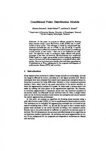
There are classes of images that exhibit features which are only found in some instances and not others. Examples include face images which may or may not show moustaches and/or glasses and histological sections, in which structures may appear in a proportion of contiguous slices in a stack. The particular example that led to the approach described here is the study of electron microscope images of nerve capillaries. There are several concentric layers of structures in capillary cross-sections (figure 1). The central region is the lumen: the space through which blood cells pass; this is surrounded by a layer of endothelial cells, and then the basement membrane. In disease condition, such as diabetic neuropathy, changes occur in the normal structure of the capillaries, including constriction of the lumen. In some cases the lumen can become so constricted as to be unidentifiable (figure 1(b)). Finding the boundaries between these structures is important in quantifying disease status and we have approached this task using Active Shape Models and Genetic Search for the Basement Membrane / Endothelial Cell (BMEC) boundary [6]. The lumen boundary is potentially easier to locate due to the clearer contrast, but in modelling it we need to take account of the fact that it is often missing. To use Active Shape Model search we need to build Point Distribution Models (PDMs) of all the structures in the capillaries, including the lumen, when it is present. We have considered three possibilities for dealing with the intermittent presence of the lumen: Separate models for capillaries with and without a visible
33
(a)
(b)
Figure 1: Examples from the set of diabetic nerve capillary data
lumen; a Segmented model in which each separate boundary has a flag for presence or absence; or a Single model in which each point is flagged for inclusion or exclusion individually. We prefer the third option as it allows us more flexibility in admitting arbitrary patterns of inclusion, and is more likely to capture the relationships between different components, for example, the gradual inclusion of a new feature across a stack of histological slices. The difficulty presented by this approach is in training a PDM with arbitrarily missing data points.
2
Data Imputation
Our approach to building models with arbitrarily missing data points is to include in the PDM the coordinates of those boundary points that are present, and to estimate the positions of the points that are not represented in some examples. This problem of data imputation - estimating missing data values - is a fairly common one in statistical applications, and a number of methods have been proposed (Rubin [5]). In adopting a method, our goal is to end up with a PDM (means and eigenvectors of the point positions) as close as possible to those we would have obtained had all the data been available. In this section we describe our own, novel, method of data imputation and evaluate its performance in comparison with three other well-founded methods with a view to their suitability for PDM building.
2.1
Imputation Methods
Replacement with mean: The simplest method is to replace each missing value with the mean of the values that are present. This clearly underestimates the variance in the data – a serious disadvantage for building PDMs. Principal Component Analysis: Dear [4] proposed an imputation technique in which initial imputation with the means is then re-estimated using the first principal component of the imputed data. In this way, gross trends in the data are preserved.
34
Maximum Likelihood : Beale and Little [1] present an iterative method to produce a maximum likelihood estimate of the missing values using a form of the Expectation Maximisation (EM) algorithm. Before this algorithm can begin, an initial estimate of the missing data must be generated. A sensible initial value is the mean over all available data. The algorithm can be extremely sensitive to the quality of this initial estimate as is shown in the evaluation in section 2.2. Iterated PCA: We have developed a further method of imputation, designed to retain data characteristics required by a subsequent PCA carried out on the imputed data. Specifically, we wish to impute values in such a way as to retain relationships found in the original data and do this without reducing the total variance. The algorithm is based on an iterative version of Dear’s [4] PCA imputation with several modifications and can be described with the following equations: 2 (Pxm , µx , σxm , bxm ) = pca(x, m)
(1)
x ˆ = µx + bxm Pxm T , xi.Mi = x ˆi.Mi
(2)
where x is the original data, xij is the j th observed value in example i, Mi is the set of variables missing in example i, xi.Mi is the set of estimated missing values from xi and pca is a function that computes the first m principle components 2 (Pxm ), the variance each mode represents (σxm ) and the mean (µx ) of x, together with the associated reconstruction parameters (bxm ) for each example. We begin by initialising x, for which we use mean value imputation, and cycle through equations 1-2 until convergence. Choosing the value of m is crucial to the well-mannered convergence of the algorithm. We use the following scheme: m is set to 1 and the algorithm is run to convergence. The imputed data is now consistent with data patterns represented by the first mode of variation, but no others. To include relationships represented by other modes we increase m by 1 and repeat the convergence, starting at the result of the previous iteration. At each stage of the iteration we are including effects of higher modes in the imputed data, and matching it more closely to the original data patterns. However, the imputed data itself also has some influence on the modes produced by PCA. As we continue to include higher modes we will eventually reach one which is mainly influenced by the effect of the imputed data, after which the algorithm will not converge. Rather, the imputed data would be updated to reinforce the effects of earlier imputed data. We therefore need a stopping criterion. In our experiments we continue iterating until : P 2 σ P xm >p (3) σx2 where σx2 is the variance of all modes of x and p is the proportion of complete data examples. This stopping criterion is somewhat heuristic, and has not been shown to be optimal. However, it leads to satisfactory performance in the evaluation experiments.
35
2.2
Evaluation of Imputation Methods
Each of the imputation methods described in section 2.1 was evaluated using synthesised data and some real shape data from annotated capillary boundaries. Synthetic data: fifty vectors, each with ten elements, were constructed using the following algorithm: for i = 1 to 50 xi = (i, 2i, 3i, ..., 10i); xi = xi + ir; x = concat xi with x The intention of this data is to evaluate the ability of an imputation method to retain the underlying relationships in the data. There is one consistent relationship for each vector, namely the increment in successive values, proportional to the first element. The relationship is not perfect, being perturbed by the random factor r (between -0.5 and 0.5), also scaled by the first element in each vector, i. These vectors do not represent shapes, but give an insight into the effectiveness of the methods in reconstructing patterns in the data corrupted by noise and missing elements. Nerve capillary landmark data: Here we use a subset of 30 examples of the marked-up BMEC boundaries from capillary images. We take the first 30 points in each case. This data gives an insight into the performance of the imputation methods on realistic data. Evaluation tests: In each case we remove a proportion (varying between 1% and 50%) of the data points and replace them with imputed values according to each of the four schemes. To measure the effectiveness of the imputation we make two measures on the resulting data. Firstly we measure the Euclidean distance (in the vector space of the data) between each example and its imputed version, giving a measure of the raw error in the imputation process. Secondly, as we are interested in preserving the modes of variation of the original data we measure the Euclidean distance between the corresponding eigenvectors of the original and imputed data sets. In the case of the synthetic data, there is only one significant mode of variation, and only one eigenvector. In the case of the capillary data, we estimate this distance for the first three eigenvectors. For the synthetic data, there is a third measure we can make. In this case we know the underlying ”ideal” relationship between the elements of each vector before corruption by randomisation. It is interesting to see how well the imputation process reconstructs this underlying relationship in the presence of the noise. We therefore measure the distance between the ideal vector and the imputed vector in each case. Results of the evaluation are shown in figure 2.2. The iterated PCA method gives the closest imputation to the original data in both cases. For the synthetic example, the maximum likelihood (EM) method gives almost identical results (fig 2(a)). In the case of the capillary data (fig 2(b)), however, the PCA method comes closest to the performance of iterated PCA, though noticeably worse at higher proportions of imputed data. In calculating the distance between the raw and imputed eigenvectors, both iterated PCA and EM again perform equivalently, and much better than the other methods, and PCA and iterated PCA give similar performance on the capillary data. The maximum likelihood estimates for imputation are influenced strongly by the initial estimates of the missing data (in this case the mean values). This is a poor estimate in the case of the capillary data and
36
results in the poor performance in this case. The structure in the variation of Euclidean distance between imputed and original modes of variation, with increasing proportion of imputation, seen in figures 2(c) and 2(d), is due to the significant effect that small changes can have on an eigen-analysis of the data. Figure 2(e) shows the difference between the ”ideal” synthetic data and the imputed values after randomisation. The distance between the ”raw” randomised data and the underlying data is, of course, independent of the quantity of imputation being applied and therefore constant. Both the EM and iterated PCA methods retain a good estimate of this distance in the presence of up to 50% imputation, and therefore seem to be responding to underlying patterns in the data. The other methods, as might be expected from figures 2(c) and 2(e), do not. Figure 2(f) shows the difference in total variance between the original and imputed capillary data. The iterated PCA method retains the total variance of the data even in the presence of large amounts of missing data. The other methods all perform poorly on this measure. The iterated PCA method appears to have the desired properties of an imputation scheme. Other methods also have these properties for one or other of the test cases, but not both. Mean imputation was always, of course, unlikely to meet our criteria, but has been included to give a yardstick for measuring inadequate performance.
3
Modelling Shape and Structure
Here we describe how we combine data imputation with a model of structural variation. As our models constitute a variant of PDMs we call them Structured Point Distribution Models (SPDMs).
3.1
Building the models
The modifications that need to be made to a standard PDM to deal with intermittent structures are the following. We build a model that assumes all points are represented (our capillary model would assume a lumen, a face model might assume the presence of a moustache). When a PDM landmark point is not represented in a particular image it is replaced by a placeholder (such as NaN - a computational representation of Not a Number). Once the training set has been assembled, the shapes are aligned using the data points that are available, and the missing data values imputed by some imputation scheme (we prefer iterated PCA, of course). So an initial training vector for a shape i represented by points [(x1 , y1 ), (x2 , y2 ), (x3 , y3 ), (x4 , y4 )] where (x3 , y3 ) is unobserved, is represented as T the data vector: xi = (x1 , x2 , N aN, x4 , y1 , y2 , N aN, y4 ) . Following alignment and imputation of missing values we get a new shape vector (primed elements T ˆ3 , x04 , y10 , y20 , yˆ3 , y40 ) . Shape are aligned, hat elements are imputed): x ˆ0i = (x01 , x02 , x parameters, bs are then calculated by PCA in the usual way [3]. While this gives us a model of shape that represents as closely as possible the shape variation we observe in the entire structure, we have lost the structural information about which boundary points may or may not be missing. We therefore
37
Distance of imputed data from original data
Distance of imputed data from original data 450
180 EM PCA iterated PCA Mean
140 120 100 80 60 40
350 300 250 200 150 100 50
20 0
EM PCA iterated PCA Mean
400
Mean distance per example
Mean distance per example
160
0
10
20 30 % data missing
40
0
50
0
10
20 30 % data missing
(a)
40
50
(b) Distance of first 3 imputed modes from original modes
Distance of imputed modes from original modes 1.4
0.25 EM PCA iterated PCA Mean
0.2
EM PCA iterated PCA Mean
1.2
Mode distance
Mode distance
1
0.15
0.1
0.8 0.6 0.4
0.05 0.2
0
0
0
10
20 30 % data missing
40
50
0
10
20 30 % data missing
(c) 5
Ideal EM PCA iterated PCA Mean
120 100 80 60 40
−5
−10
EM PCA iterated PCA Mean
−15
20 0
−20
0
10
Difference in total variance
x 10
0
Variance difference
Mean distance per example
140
50
(d) 4
Distance of imputed data from perfect data 180 160
40
20 30 % data missing
40
50
(e)
0
10
20 30 % data missing
40
50
(f)
Figure 2: Imputation performance. (a),(c),(e) – synthetic data, (b),(d),(f) – capillary images. Error is shown as a function of increasing proportion of imputed data. (a),(b) – raw error. (c),(d) – error in principal components. (e) error in capturing the ”ideal” data pattern. (f) difference in total variance (see text).
(a)
(b)
Figure 3: Synthetic shape. (a) examples from the set of synthetic training data. (b) the first mode of variation.
38
augment the shape vector with a binary structure vector. For our shape i above T with point 3 missing the structure vector would be: xsi = (1, 1, 0, 1) . This gives us a representation of the structure containing significant redundancy, but which allows for arbitrary patterns of inclusion or exclusion of landmark points in the model. This redundancy can be reduced using PCA, just as in the case of classical PDMs. The modes of the PCA represent the relationships between the structures in the landmark data. In the case of the capillary boundaries the analysis results in a single mode, containing almost all the variance, representing the presence or absence of the lumen at its extremes. We have therefore reduced our structure vector to a parameter vector of length 1. The SPDM like the PDM is a generative model; that is, given a parameter vector we can recreate the structure vector for a particular instance. The disadvantage of this approach is that we are representing a binary process (presence or absence) by a linear model. To recover binary parameters in the reconstructed structure vector we threshold the individual elements. We use a threshold that represents the probability that a particular feature point will be present in the image. The PCA of the structural data matrix xs results in a matrix of continuous structure parameters bd , which can then be used, together with the shape parameters bs to build the combined model of shape and structure. This is done in a way similar to the construction of Active Appearance Models [2]. For each training example we generate a concatenated vector: µ ¶ ˆ bs b= (4) bd where ˆ bs is a matrix of shape parameters generated after first shifting and scaling the input (imputed) data to lie between 0 and 1. We perform this scaling to avoid problems associated with shape and structure being measured on different scales. In choosing to perform this transformation on the data, we are effectively treating shape and structure as equally important. A combined model of shape and structure is obtained by a further application of PCA. c ≈ Qb
(5)
where Q is a matrix of t eigenvectors expressing the correlations between the shape and structure data in vector b and c is a vector of combined model parameters which controls both the shape and structure of the data. We can obtain b from c: b = QT c
(6)
From these equations we can produce the shape and structure vector of any shape represented by the model.
3.2
Evaluation
We evaluate our approach to shape and structure modelling using a synthetic shape set, nerve capillary images and face images. Firstly we demonstrate that presence or absence of structure is represented in the model, and that correlations with
39
shape data are captured. Secondly we demonstrate that modelling the presence or absence of structures increases the specificity of the model. Synthetic data: A set of synthetic shapes was generated using the following algorithm. generate a random number r, between 10 and 30 form a kite from the points [(r, 50), (50, 90), (100, 50), (50, 10)] if (r < 25) form a square, centred (50, 50), with side length 100 − 2r otherwise put 4 N aN values in the data vector This generates a set of structures consisting of squares within kites (see figure 2). The first coordinate of the kite and the size of the square are correlated. When the size of the inner square would be less than 0 the feature is not present in the image. The proportion of complete to incomplete structures is 5:1. The SPDM built from 50 training examples, retaining 99.5% of variation has only one mode of variation shown in figure 2(a). The shape model has captured the correlation between the size of the square and the shape of the kite, and the thresholding of the structure vector has removed it at the relevant places. Nerve Capillaries: An SPDM was calculated from 38 nerve capillary images, 15 of which contained lumens so constricted that they are practically undetectable, so that only the BMEC boundary was annotated. Examples of the shapes are shown in figure 4(a). The 99.5% of data retained produced 6 modes of variation, the first three of which are shown in figure 4(b). Note that all the structural information is contained in the first mode of the model. The second expresses lumen constriction and the third appears to be capturing the translation of the lumen within the capillary. Faces: Figure 3.2(a) shows some examples from a set of 29 face images marked up with 33 landmarks on the face outline, eyes nostrils and moustache (present in nine out of the 29 faces). Figure 3.2(b) shows the first two modes of variation. Once again the first mode represents the structural variation and the others represent shape variation. Model Specificity: The inclusion of the lumen structure into the model of nerve capillaries is intended to contribute additional constraints to the model during search, i.e. to increase its specificity. To measure the specificity of the models, we used the 38 training examples of capillaries and 29 face images to build SPDMs and PDMs retaining 99.5% of observed variability in each case. From each training set we created increasingly invalid shapes by randomly perturbing the point positions in the training examples using the following algorithm. for i=1 to 25 for each training example x ¯ xr ; b = Qxr ; x ˆir = QT b xir = x + i100 This creates, for each training example, twenty five increasingly invalid shapes obtained by adding a random shift to each point. If we try to fit the model to the invalid data, a highly specific (constrained) model will find the nearest valid shape, whereas a less- specific model will fit more closely to the invalid example. For our purposes, we measure closeness as the mean point to point distance between the model fit landmarks and the corresponding annotation landmark.
40
Figure 5 shows the fits of SPDM and PDM models of capillaries and faces to the unperturbed(valid) and perturbed(invalid) data, with increasing random perturbation. In each case the model shows some specificity by fitting more closely to the nearest valid example than the perturbed version. However, for both capillary and face shapes, the effect is more marked for the SPDM, indicating increased specificity of the structural model.
4
Conclusions and Discussion
We have presented an extension to Point Distribution Modelling to deal with circumstances in which features of the objects to be modelled may be wholly present or absent in a proportion of examples. Our method combines the use of a structure vector, which is subject to the same statistical analysis as the shape vector, and imputation of values for model points which are coded as absent in the structure vector. We have developed a straightforward method for imputation which causes minimal distortion to the distributions of shapes in the original data. Using experiments on synthesised data and data from real images we have shown that the Structured Point Distribution Models successfully capture the variation in shape and structure present in an image set and the correlations among these, and that the use of the structured models improves the specificity of the model over the classical PDM. Although not demonstrated in this short paper, the method can be applied to Appearance Models [2] also, and model the grey level appearance of intermittently present features.
References [1] E M L Beale and R J A Little. Missing values in multivariate analysis. 1975. [2] T F Cootes, G J Edwards, and Taylor. Active appearance models. In Proceedings of the European Conference on Computer Vision, volume 2, pages 484–498, 1998. [3] T F Cootes, C J Taylor, D H Cooper, and J Graham. Active Shape Models - their training and application. Computer Vision and Image Understanding, 61(1):38–59, January 1995. [4] R E Dear. A principle-component missing data method for multiple regression models. Technical Report Report SP-86, 1959. [5] R J A Little and D B Rubin. Statistical Anaylsis with Missing Data. Wiley, New York, USA, 1987. [6] M Rogers, J Graham, and R A Malik. Exploiting weak shape constraints to segment capillary images in microangiopathy. In Proceedings of the 3 rd International Conference on Medical Image Computing and Computer-Assisted Intervention, pages 717–726, Pittsburg, PA, USA, October 2000.
41
(a)
1 (b) 2
Figure 4: Faces. (a) examples from the set of face shape training data. (b) first two modes of variation. Note that the first mode encapsulates the structure of the missing data. (a)
1
(b) 2
3
Figure 5: Capillaries. (a) examples from the set of nerve capillary training data. (b) the first three of six modes. Note that the first mode encapsulates the structure of the missing data. Model Specificity Mean euclidian distance per landmark (pixels)
Mean euclidian distance per landmark (pixels)
Model Specificity 25 SPDM −> annotation SPDM −> random PDM −> annotation PDM −> random
20
15
10
5
0
0
5
10
15
20
25
35 SPDM −> annotation SPDM −> random PDM −> annotation PDM −> random
30 25 20 15 10 5 0
0
5
10
15
i
i
(a)
(b)
20
25
Figure 6: The curves show the mean point to point landmark distance for both PDM and SPDM model fits to the original shape (annotations) and perturbed examples (random). (a) capillaries, (b) faces.
42