Structured prediction models for RNN based

Structured prediction models for RNN based sequence labeling in clinical text Abhyuday N Jagannatha1 , Hong Yu1,2 1 University of Massachusetts, MA, USA 2 Bedford VAMC and CHOIR, MA, USA [email protected] , [email protected]

1

Abstract

from drug efficacy analysis to adverse effect surveillance.

Sequence labeling is a widely used method for named entity recognition and information extraction from unstructured natural language data. In the clinical domain one major application of sequence labeling involves extraction of relevant entities such as medication, indication, and side-effects from Electronic Health Record Narratives. Sequence labeling in this domain presents its own set of challenges and objectives. In this work we experiment with Conditional Random Field based structured learning models with Recurrent Neural Networks. We extend the previously studied CRF-LSTM model with explicit modeling of pairwise potentials. We also propose an approximate version of skip-chain CRF inference with RNN potentials. We use these methods1 for structured prediction in order to improve the exact phrase detection of clinical entities.

A widely used method for Information Extraction from natural text documents involves treating the text as a sequence of tokens. This format allows sequence labeling algorithms to label the relevant information that should be extracted. Several sequence labeling algorithms such as Conditional Random Fields (CRFs), Hidden Markov Models (HMMs), Neural Networks have been used for information extraction from unstructured text. CRFs and HMMs are probabilistic graphical models that have a rich history of Natural Language Processing (NLP) related applications. These methods try to jointly infer the most likely label sequence for a given sentence.

Introduction

Patient data collected by hospitals falls into two categories, structured data and unstructured natural language texts. It has been shown that natural text clinical documents such as discharge summaries, progress notes, etc are rich sources of medically relevant information like adverse drug events, medication prescriptions, diagnosis information etc. Information extracted from these natural text documents can be useful for a multitude of purposes ranging 1

Code is available at https://github.com/abhyudaynj/LSTMCRF-models

Recently, Recurrent (RNN) or Convolutional Neural Network (CNN) models have increasingly been used for various NLP related tasks. These Neural Networks by themselves however, do not treat sequence labeling as a structured prediction problem. Different Neural Network models use different methods to synthesize a context vector for each word. This context vector contains information about the current word and its neighboring content. In the case of CNN, the neighbors comprise of words in the same filter size window, while in Bidirectional-RNNs (Bi-RNN) they contain the entire sentence. Graphical models and Neural Networks have their own strengths and weaknesses. While graphical models predict the entire label sequence jointly, they usually rely on special hand crafted features to provide good results. Neural Networks (especially Re-

856 Proceedings of the 2016 Conference on Empirical Methods in Natural Language Processing, pages 856–865, c Austin, Texas, November 1-5, 2016. 2016 Association for Computational Linguistics

current Neural Networks), on the other hand, have been shown to be extremely good at identifying patterns from noisy text data, but they still predict each word label in isolation and not as a part of a sequence. In simpler terms, RNNs benefit from recognizing patterns in the surrounding input features, while structured learning models like CRF benefit from the knowledge about neighboring label predictions. Recent work on Named Entity Recognition by (Huang et al., 2015) and others have combined the benefits of Neural Networks(NN) with CRF by modeling the unary potential functions of a CRF as NN models. They model the pairwise potentials as a paramater matrix [A] where the entry Ai,j corresponds to the transition probability from the label i to label j. Incorporating CRF inference in Neural Network models helps in labeling exact boundaries of various named entities by enforcing pairwise constraints. This work focuses on labeling clinical events (medication, indication, and adverse drug events) and event related attributes (medication dosage, route, etc) in unstructured clinical notes from Electronic Health Records. Later on in the Section 4, we explicitly define the clinical events and attributes that we evaluate on. In the interest of brevity, for the rest of the paper, we use the broad term “Clinical Entities” to refer to all medically relevant information that we are interested in labeling. Detecting entities in clinical documents such as Electronic Health Record notes composed by hospital staff presents a somewhat different set of challenges than similar sequence labeling applications in the open domain. This difference is partly due to the critical nature of medical domain, and partly due to the nature of clinical texts and entities therein. Firstly, in the medical domain, extraction of exact clinical phrase is extremely important. The names of clinical entities often follow polynomial nomenclature. Disease names such as Uveal melanoma or hairy cell leukemia need to be identified exactly, since partial names ( hairy cell or melanoma) might have significantly different meanings. Additionally, important clinical entities can be relatively rare events in Electronic Health Records. For example, mentions of Adverse Drug Events occur once every six hundred words in our corpus. CRF inference with NN models cited previously do improve exact 857

phrase labeling. However, better ways of modeling the pairwise potential functions of CRFs might lead to improvements in labeling rare entities and detecting exact phrase boundaries. Another important challenge in this domain is a need to model long term label dependencies. For example, in the sentence “the patient exhibited A secondary to B”, the label for A is strongly related to the label prediction of B. A can either be labeled as an adverse drug reaction or a symptom if B is a Medication or Diagnosis respectively. Traditional linear chain CRF approaches that only enforce local pairwise constraints might not be able to model these dependencies. It can be argued that RNNs may implicitly model label dependencies through patterns in input features of neighboring words. While this is true, explicitly modeling the long term label dependencies can be expected to perform better. In this work, we explore various methods of structured learning using RNN based feature extractors. We use LSTM as our RNN model. Specifically, we model the CRF pairwise potentials using Neural Networks. We also model an approximate version of skip chain CRF to capture the aforementioned long term label dependencies. We compare the proposed models with two baselines. The first baseline is a standard Bi-LSTM model with softmax output. The second baseline is a CRF model using handcrafted feature vectors. We show that our frameworks improve the performance when compared to the baselines or previously used CRF-LSTM models. To the best of our knowledge, this is the only work focused on usage and analysis of RNN based structured learning techniques on extraction of clinical entities from EHR notes.

2

Related Work

As mentioned in the previous sections, both Neural Networks and Conditional Random Fields have been widely used for sequence labeling tasks in NLP. Specially, CRFs (Lafferty et al., 2001) have a long history of being used for various sequence labeling tasks in general and named entity recognition in particular. Some early notable works include McCallum et. al. (2003), Sarawagi et al. (2004) and Sha et. al. (2003). Hammerton et. al. (2003) and Chiu et. al. (2015) used Long Short Term Memory (LSTM)

(Hochreiter and Schmidhuber, 1997) for named entity recognition. Several recent works on both image and text based domains have used structured inference to improve the performance of Neural Network based models. In NLP, Collobert et al (2011) used Convolutional Neural Networks to model the unary potentials. Specifically for Recurrent Neural Networks, Lample et al. (2016) and Huang et. al. (2015) used LSTMs to model the unary potentials of a CRF. In biomedial named entity recognition, several approaches use a biological corpus annotated with entities such as protein or gene name. Settles (2004) used Conditional Random Fields to extract occurrences of protein, DNA and similar biological entity classes. Li et. al. (2015) recently used LSTM for named entity recognition of protein/gene names from BioCreative corpus. Gurulingappa et. al. (2010) evaluated various existing biomedical dictionaries on extraction of adverse effects and diseases from a corpus of Medline abstracts. This work uses a real world clinical corpus of Electronic Health Records annotated with various clinical entities. Jagannatha et. al. (2016) recently showed that RNN based models outperform CRF models on the task of Medical event detection on clinical documents. Other works using a real world clinical corpus include Rochefort et al. (2015), who worked on narrative radiology reports. They used a SVM-based classifier with bag of words feature vector to predict deep vein thrombosis and pulmonary embolism. Miotto et. al. (2016) used a denoising autoencoder to build an unsupervised representation of Electronic Health Records which could be used for predictive modeling of patient’s health.

3

Methods

We evaluate the performance of three different BiLSTM based structured prediction models described in section 3.2, 3.3 and 3.4. We compare this performance with two baseline methods of Bi-LSTM(3.1) and CRF(3.5) model. 3.1

Bi-LSTM (baseline)

This model is a standard bidirectional LSTM neural network with word embedding input and a Softmax Output layer. The raw natural language input 858

sentence is processed with a regular expression tokenizer into sequence of tokens x = [xt ]T1 . The token sequence is fed into the embedding layer, which produces dense vector representation of words. The word vectors are then fed into a bidirectional RNN layer. This bidirectional RNN along with the embedding layer is the main machinery responsible for learning a good feature representation of the data. The output of the bidirectional RNN produces a feature vector sequence ω(x) = [ω(x)]T1 with the same length as the input sequence x. In this baseline model, we do not use any structured inference. Therefore this model alone can be used to predict the label sequence, by scaling and normalizing [ω(x)]T1 . This is done by using a softmax output layer, which scales the output for a label l where l ∈ {1, 2, ..., L} as follows: exp(ω(x)t Wj ) P (˜ yt = j|x) = PL l=1 exp(ω(x)t Wl )

(1)

The entire model is trained end-to-end using categorical cross-entropy loss. 3.2

Bi-LSTM CRF

This model is adapted from the Bi-LSTM CRF model described in Huang et. al. (2015). It combines the framework of bidirectional RNN layer[ω(x)]T1 described above, with linear chain CRF inference. For a general linear chain CRF the probability of a label sequence y˜ for a given sentence x can be written as : N 1 Y P (˜ y |x) = exp{φ(˜ yt ) + ψ(˜ yt , y˜t+1 )} Z

(2)

t=1

Where φ(yt ) is the unary potential for the label position t and ψ(yt , yt+1 ) is the pairwise potential between the positions t,t+1. Similar to Huang et. al. (2015), the outputs of the bidirectional RNN layer ω(x) are used to model the unary potentials of a linear chain CRF. In particular, the NN based unary potential φnn (yt ) is obtained by passing ω(x)t through a standard feed-forward tanh layer. The binary potentials or transition scores are modeled as a matrix [A]L×L . Here L equals the number of possible labels including the Outside label. Each element Ai,j represents the transition score from label i to j. The

probability for a given sequence y˜ can then be calculated as :

Labels ADE Indication Other SSD Severity Drugname Duration Dosage Route Frequency

T 1 Y exp{φnn (˜ yt ) + Ay˜t ,˜yt+1 } (3) P (˜ y |x; θ) = Z t=1

The network is trained end-to-end by minimizing the negative log-likelihood of the ground truth label sequence ˆy for a sentence x as follows: XX δ(yt = yˆt ) log P (yt |x; θ)} L(x, ˆy; θ) = − t

yt

(4) The negative log likelihood of given label sequence for an input sequence is calculated by sumproduct message passing. Sum-product message passing is an efficient method for exact inference in Markov chains or trees. 3.3

Bi-LSTM CRF with pairwise modeling

In the previous section, the pairwise potential is calculated through a transition probability matrix [A] irrespective of the current context or word. For reasons mentioned in section 1, this might not be an effective strategy. Some clinical entities are relatively rare. Therefore transition from an Outside label to a clinical label might not be effectively modeled by a fixed parameter matrix. In this method, the pairwise potentials are modeled through a nonlinear Neural Network which is dependent on the current word and context. Specifically, the pairwise potential ψ(yt , yt+1 ) in equation 2 is computed by using a one dimensional CNN with 1-D filter size 2 and tanh non-linearity. At every label position t, it takes [ω(x)t ; ω(x)t+1 ] as input and produces a L×L pairwise potential output ψnn (yt , yt+1 ). This CNN layer effectively acts as a non-linear feed-forward neuron layer, which is repeatedly applied on consecutive pairs of label positions. It uses the output of the bidirectional LSTM layer at positions t and t + 1 to prepare the pairwise potential scores. The unary potential calculation is kept the same as in Bi-LSTM-CRF. Substituting the neural network based pairwise potential ψnn (yt , yt+1 ) into equation 2 we can reformulate the probability of the label sequence y˜ given the word sequence x as : P (˜ y |x; θ) =

N 1 Y exp{φnn (˜ yt ) + ψnn (˜ yt , y˜t+1 )} Z t=1 (5)

859

Num. of Instances 1807 3724 40984 3628 17008 926 5978 2862 5050

Avg word length ± std 1.68 ± 1.22 2.20 ± 1.79 2.12 ± 1.88 1.27 ± 0.62 1.21 ± 0.60 2.01 ± 0.74 2.09 ± 0.82 1.20± 0.47 2.44± 1.70

Table 1: Annotation statistics for the corpus.

The neural network is trained end-to-end with the objective of minimizing the negative log likelihood in equation 4. The negative log-likelihood scores are obtained by sum-product message passing. 3.4

Approximate Skip-chain CRF

Skip chain models are modifications to linear chain CRFs that allow long term label dependencies through the use of skip edges. These are basically edges between label positions that are not adjacent to each other. Due to these skip edges, the skip chain CRF model (Sutton and McCallum, 2006) explicitly models dependencies between labels which might be more than one position apart. The joint inference over these dependencies are taken into account while decoding the best label sequence. However, unlike the two models explained in the preceding section, the skip-chain CRF contains loops between label variables. As a result we cannot use the sum-product message passing method to calculate the negative log-likelihood.The loopy structure of the graph in skip chain CRF renders exact message passing inference intractable. Approximate solutions for these models include loopy belief propagation(BP) which requires multiple iterations of message passing. However, an approach like loopy BP is prohibitively expensive in our model with large Neural Net based potential functions. The reason for this is that each gradient descent iteration for a combined RNN-CRF model requires a fresh calculation of the marginals. In one approach to mitigate this, Lin et. al. (2015) directly model the messages in the message passing inference of a 2-D grid CRF for image segmentation. This bypasses the need for modeling the potential function, as well as calculating the ap-

proximate messages on the graph using loopy BP. Approximate CRF message passing inference: Lin et. al. (2015) directly estimate the factor to variable message using a Neural Network that uses input image features. Their underlying reasoning is that the factor-to-variable message from factor F to label variable yt for any iteration of loopy BP can be approximated as a function of all the input variables and previous messages that are a part of that factor. They only model one iteration of loopy BP, and empirically show that it leads to an appreciable increase in performance. This allows them to model the messages as a function of only the input variables, since the messages for the first iteration of message passing are computed using the potential functions alone. We follow a similar approach for calculation of variable marginals in our skip chain model. However, instead of estimating individual factor-tovariable messages, we exploit the sequence structure in our problem and estimate groups of factorto-variable messages. For any label node yt , the first group contains factors that involve nodes which occur before yt in the sentence (from left). The second group of factor-to-variable messages corresponds to factors involving nodes occurring later in the sentence. We use recurrent computational units like LSTM to estimate the sum of log factor-to-variable messages within a group. Essentially, we use bidirectional recurrent computation to estimate all the incoming factors from left and right separately. To formulate this, let us assume for now that we are using skip edges to connect the current node t to m preceding and m following nodes. Each edge, skip or otherwise, is denoted by a factor which contains the binary potential of the edge and the unary potential of the connected node. As mentioned earlier, we will divide the factors associated with node t into two sets, FL (t) and FR (t). Here FL (t) , contains all factors formed between the variables from the group {yt−m , ..., yt−1 } and yt . So we can formulate the combined message from factors in FL (t) as X βL (yt ) = [ βF →t (yt )] (6) F ∈FL (t)

The combined messages from factors in FR (t) which contains variables from yt+1 to yt+m can be 860

formulated as : X

βR (yt ) = [

F ∈FR (t)

βF →t (yt )]

(7)

We also need the unary potential of the label variable t to compose its marginal. The unary potentials of each variable from {yt−m , ..., yt−1 } and {yt+1 , ..., yt+m } should already be included in their respective factors. The log of the unnormalized marginal P¯ (yt |x) for the variable yt , can therefore be calculated by log P¯ (yt |x) = βR (yt ) + βL (yt ) + φ(yt )

(8)

Similar to Lin et. al. (2015), in the interest of limited network complexity, we use only one message passing iteration. In our setup, this means that a variable-to-factor message from a neighboring variable yi to the current variable yt contains only the unary potentials of yi and binary potential between yi , yt . As a consequence of this, we can see that βL (yt ) can be written as : βL (yt ) =

t−m X

log

i=t−1

X

[exp ψ(yt , yi ) + φ(yi )] (9)

yi

Similarly, we can formulate a function for βR (yt ) in a similar way : βR (yt ) =

t+m X

i=t+1

log

X

[exp ψ(yt , yi ) + φ(yi )]

yi

(10)

Modeling the messages using RNN: As mentioned previously in equation 8, we only need to estimate βL (yt ), βR (yt ) and φ(yt ) to calculate the marginal of variable yt . We can use φnn (yt ) framework introduced in section 3.2 to estimate the unary potential for yt . We use different directions of a bidirectional LSTM to estimate βR (yt ) and βL (yt ). This eliminates the need to explicitly model and learn pairwise potentials for variables that are not immediate neighbors. The input to this layer at position t is [φnn (yt ); ψnn (yt , yt+1 )] (composed of potential functions described in section 3.3). This can be viewed as an LSTM layer aggregating beliefs about yt from the unary and binary potentials of [y]t−1 1

Models CRF Bi-LSTM Bi-LSTM CRF Bi-LSTM CRF-pair Approximate Skip-Chain CRF

Strict Evaluation ( Exact Match) Recall Precision F-score 0.7385 0.8060 0.7708 0.8101 0.7845 0.7971 0.7890 0.8066 0.7977 0.8073 0.8266 0.8169 0.8364 0.8062 0.8210

Relaxed Evaluation (Word based) Recall Precision F-score 0.7889 0.8040 0.7964 0.8402 0.8720 0.8558 0.8068 0.8839 0.8436 0.8245 0.8527 0.8384 0.8614 0.8651 0.8632

Table 2: Cross validated micro-average of Precision, Recall and F-score for all clinical tags

to approximate the sum of messages from left side βL (yt ). Similarly, βR (yt ) can be approximated from the LSTM aggregating information from the opposite direction. Formally, βL (yt ) is approximated as a function of neural network based unary and binary potentials as follows: βL (yt ) ≈ f ([φnn (yi ); ψnn (yi , yi+1 )]1t−1 )

(11)

Using LSTM as a choice for recurrent computation here is advantageous, because LSTMs are able to learn long term dependencies. In our framework, this allows them to learn to prioritize more relevant potential functions from the sequence [[φnn (yi ); ψnn (yi , yi+1 )]t−1 1 . Another advantage of this method is that we can approximate skip edges between all preceding and following nodes, instead of modeling just m surrounding ones. This is because LSTM states are maintained throughout the sentence. The partition function for yt can be easily obtained by using logsumexp over all label entries of the unnormalized log marginal shown in equation 8 as follows: X Zt = exp[βR (yt ) + βL (yt ) + φ(yt )] (12) yt

Here the partition function Z is a different for different positions of t. Due to our approximations, it is not guaranteed that the partition function calculated from different marginals of the same sentence are equal. The normalized marginal can be now calculated by normalizing log P¯ (yt |x) in equation 8 using Zt . L(x, ˆy; θ) = −

XX t

δ(yt = yˆt )(βR (yt ; θ)

yt

(13)

+βL (yt ; θ) + φ(yt ; θ) − log Zt (θ)) 861

The model is optimized using cross entropy loss between the true marginal and the predicted marginal. The loss for a sentence x with a ground truth label sequence ˆy is provided in equation 13. 3.5

CRF (baseline)

We use the linear chain CRF, which is a widely used model in extraction of clinical named entities. As mentioned previously, Conditional Random Fields explicitly model dependencies between output variables conditioned on a given input sequence. The main inputs to CRF in this model are not RNN outputs, but word inputs and their corresponding word vector representations. We add additional sentence features consisting of four vectors. Two of them are bag of words representation of the sentence sections before and after the word respectively. The remaining two vectors are dense vector representations of the same sentence sections. The dense vectors are calculated by taking the mean of all individual word vectors in the sentence section. We add these features to explicitly mimic information provided by the bidirectional chains of the LSTM models.

4

Dataset

We use an annotated corpus of 1154 English Electronic Health Records from cancer patients. Each note was annotated2 by two annotators who label clinical entities into several categories. These categories can be broadly divided into two groups, Clinical Events and Attributes. Clinical events include any specific event that causes or might contribute to a change in a patient’s medical status. Attributes are phrases that describe certain important properties about the events. 2 The annotation guidelines can be found at https://github.com/abhyudaynj/LSTM-CRFmodels/blob/master/annotation.md

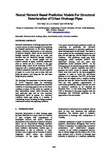
Figure 1: Plots of Recall, Precision and F-score for RNN based methods. The metrics with prefix Strict are using phrase based evaluation. Relaxed metrics use word based evaluation.Bar-plots are in order with Bi-LSTM on top and Approx-skip-chain-CRF at the bottom.

Clinical Event categories in this corpus are Adverse Drug Event (ADE), Drugname , Indication and Other Sign Symptom and Diseases (Other SSD). ADE, Indication and Other SSD are events having a common vocabulary of Sign, Symptoms and Diseases (SSD). They can be differentiated based on the context that they are used in. A certain SSD should be labeled as ADE if it can be manually identified as a side effect of a drug based on the evidence in the clinical note. It is an Indication if it is an affliction that a doctor is actively treating with a medication. Any other SSD that does not fall into the above two categories ( for e.g. an SSD in patients history) is labeled as Other SSD. Drugname event labels any medication or procedure that a physician prescribes. The attribute categories contain the following properties, Severity , Route, Frequency, Duration and Dosage. Severity is an attribute of the SSD event types , used to label the severity a disease or symptom. Route, Frequency, Duration and Dosage are attributes of Drugname. They are used to label the medication method, frequency of dosage, duration of dosage, and the dosage quantity respectively. The 862

annotation statistics of the corpus are provided in the Table 1.

5

Experiments

Each document is split into separate sentences and the sentences are tokenized into individual word and special character tokens. The models operate on the tokenized sentences. In order to accelerate the training procedure, all LSTM models use batch-wise training using a batch of 64 sentences. In order to do this, we restricted the sentence length to 50 tokens. All sentences longer than 50 tokens were split into shorter size samples, and shorter sentences were prepadded with masks. The CRF baseline model(3.5) does not use batch training and so the sentences were used unaltered. The first layer for all LSTM models was a 200 dimensional word embedding layer. In order to improve performance, we initialized embedding layer values in these models with a skip-gram word embedding (Mikolov et al., 2013). The skip-gram embedding was calculated using a combined corpus

of PubMed open access articles, English Wikipedia and an unlabeled corpus of around hundred thousand Electronic Health Records. The EHRs used in the annotated corpus are not in this unlabeled EHR corpus. This embedding is also used to provide word vector representation to the CRF baseline model. The bidirectional LSTM layer which outputs ω(x) contains LSTM neurons with a hidden size ranging from 200 to 250. This hidden size is kept variable in order to control for the number of trainable parameters between different LSTM based models. This helps ensure that the improved performance in these models is only because of the modified model structure, and not an increase in trainable parameters. The hidden size is varied in such a way that the number of trainable parameters are close to 3.55 million parameters. Therefore, the Approx skip chain CRF has 200 hidden layer size, while standard Bi-LSTM model has 250 hidden layer. Since the ω(x) layer is bidirectional, this effectively means that the Bi-LSTM model has 500 hidden layer size, while Approx skip chain CRF model has 400 dimensional hidden layer. We use dropout (Srivastava et al., 2014) with a probability of 0.50 in all LSTM models in order to improve regularization performance. We also use batch norm (Ioffe and Szegedy, 2015) between layers wherever possible in order to accelerate training. All RNN models are trained in an end-to-end fashion using Adagrad (Duchi et al., 2011) with momentum. The CRF model was trained using L-BFGS with L2 regularization. We use Begin Inside Outside (BIO) label modifiers for models that use CRF objective. We use ten-fold cross validation for our results. The documents are divided into training and test documents. From each training set fold, 20% of the sentences form the validation set which is used for model evaluation during training and for early stopping. We report the word based and exact phrase match based micro-averaged recall, precision and F-score. Exact phrase match based evaluation is calculated on a per phrase basis, and considers a phrase as positively labeled only if the phrase exactly matches the true boundary and label of the reference phrase. Word based evaluation metric is calculated on labels of individual words. A word’s predicted label is considered as correct if it matches the reference label, 863

irrespective of whether the remaining words in its phrase are labeled correctly. Word based evaluation is a more relaxed metric than phrase based evaluation.

6

Results

The micro-averaged Precision, Recall and F-score for all five models are shown in Table 2. We report both strict (exact match) and relaxed (word based) evaluation results. As shown in Table 2, the best performance is obtained by Skip-Chain CRF (0.8210 for strict and 0.8632 for relaxed evaluation). All LSTM based models outperform the CRF baseline. Bi-LSTM-CRF and Bi-LSTM-CRF-pair models using exact CRF inference improve the precision of strict evaluation by 2 to 5 percentage points. BiLSTM CRF-pair achieved the highest precision for exact-match. However, the recall (both strict and relaxed) for exact CRF-LSTM models is less than BiLSTM. This reduction in recall is much less in the Bi-LSTM-pair model. In relaxed evaluation, only the Skip Chain model has a better F-score than the baseline LSTM. Overall, Bi-LSTM-CRF-pair and Approx-Skip-Chain models lead to performance improvements. However, the standard Bi-LSTM-CRF model does not provide an appreciable increase over the baseline. Figure 1 shows the breakdown of performance for each RNN model with respect to individual clinical entity labels. CRF baseline model performance is not shown in Figure 1, because its performance is consistently lower than Bi-LSTM-CRF model across all label categories. We use pairwise t-test on strict evaluation F-score for each fold in cross validation, to calculate the statistical significance of our scores. The improvement in F-score for Bi-LSTM-CRF-pair and Approx-Skip Chain as compared to Bi-LSTM baseline is statistically significant (p < 0.01). The difference in Bi-LSTMCRF and Bi-LSTM baseline, does not appear to be statistically significant (p > 0.05). However, the improvements over CRF baseline for all LSTM models are statistically significant.

7

Discussion

Overall, Approx-Skip-Chain CRF model achieved better F-scores than CRF,Bi-LSTM and Bi-LSTM-

CRF in both strict and relaxed evaluations. The results of strict evaluation, as shown in Figure 1, are our main focus of discussion due to their importance in the clinical domain. As expected, two exact inference-based CRF-LSTM models (Bi-LSTMCRF and Bi-LSTM-CRF-pair) show the highest precision for all labels. Approx-Skip-Chain CRF’s precision is lower(due to approximate inference) but it still mostly outperforms Bi-LSTM. The recall for Skip Chain CRF is almost equal or better than all other models due to its robustness in modeling dependencies between distant labels. The variations in recall contribute to the major differences in F-scores. These variations can be due to several factors including the rarity of that label in the dataset, the complexity of phrases of a particular label, etc. We believe, exact CRF-LSTM models described here require more training samples than the baseline Bi-LSTM to achieve a comparable recall for labels that are complex or “difficult to detect”. For example, as shown in table 1, we can divide the labels into frequent ( Other SSD, Indication, Severity, Drugname, Dosage, and Frequency) and rare or sparse (Duration, ADE, Route). We can make a broad generalization, that exact CRF models (especially BiLSTM-CRF) have somewhat lower recall for rare labels. This is true for most labels except for Route, Indication, and Severity. The CRF models have very close recall (0.780,0.782) to the baseline Bi-LSTM (0.803) for Route even though its number of incidences are lower (2,862 incidences) than Indication (3,724 incidences) and Severity (3,628 incidences), both of which have lower recall even though their incidences are much higher. Complexity of each label can explain the aforementioned phenomenon. Route for instance, frequently contains unique phrases such as “by mouth” or “p.o.,” and is therefore easier to detect. In contrast, Indication is ambiguous. Its vocabulary is close to two other labels: ADE (1,807 incidences) and the most populous Other SSD (40,984 incidences). As a consequence, it is harder to separate the three labels. Models need to learn cues from surrounding context, which is more difficult and requires more samples. This is why the recall for Indication is lower for CRF-LSTM models, even though its number of incidences is higher than Route. To further support our explanation, our re864

sults show that the exact CRF-LSTM models mislabeled around 40% of Indication words as Other SSD, as opposed to just 20 % in case of the BiLSTM baseline. The label Severity is a similar case. It contains non-label-specific phrases such as “not terribly”, “very rare” and “small area,” which may explain why almost 35% of Severity words are mislabeled as Outside by the bi-LSTM-CRF as opposed to around 20% by the baseline. It is worthwhile to note that among exact CRFLSTM models, the recall for Bi-LSTM-CRF-pair is much better than Bi-LSTM-CRF even for sparse labels. This validates our initial hypothesis that Neural Net based pairwise modeling may lead to better detection of rare labels.

8

Conclusion

We have shown that modeling pairwise potentials and using an approximate version of Skip-chain inference increase the performance of the LSTM-CRF models. We also show that these models perform much better than baseline LSTM and CRF models. These results suggest that the structured prediction models are good directions for improving the exact phrase extraction for clinical entities.

Acknowledgments We thank the UMassMed annotation team: Elaine Freund, Wiesong Liu, Steve Belknap, Nadya Frid, Alex Granillo, Heather Keating, and Victoria Wang for creating the gold standard evaluation set used in this work. We also thank the anonymous reviewers for their comments and suggestions. This work was supported in part by the grant HL125089 from the National Institutes of Health (NIH). We also acknowledge the support from the United States Department of Veterans Affairs (VA) through Award 1I01HX001457. This work was also supported in part by the Center for Intelligent Information Retrieval. The contents of this paper do not represent the views of CIIR, NIH, VA or the United States Government.

References Jason PC Chiu and Eric Nichols. 2015. Named entity recognition with bidirectional lstm-cnns. arXiv preprint arXiv:1511.08308.

Ronan Collobert, Jason Weston, L´eon Bottou, Michael Karlen, Koray Kavukcuoglu, and Pavel Kuksa. 2011. Natural language processing (almost) from scratch. The Journal of Machine Learning Research, 12:2493– 2537. John Duchi, Elad Hazan, and Yoram Singer. 2011. Adaptive subgradient methods for online learning and stochastic optimization. The Journal of Machine Learning Research, 12:2121–2159. Harsha Gurulingappa, Roman Klinger, Martin HofmannApitius, and Juliane Fluck. 2010. An empirical evaluation of resources for the identification of diseases and adverse effects in biomedical literature. In 2nd Workshop on Building and evaluating resources for biomedical text mining (7th edition of the Language Resources and Evaluation Conference). James Hammerton. 2003. Named entity recognition with long short-term memory. In Proceedings of the seventh conference on Natural language learning at HLTNAACL 2003-Volume 4, pages 172–175. Association for Computational Linguistics. Sepp Hochreiter and J¨urgen Schmidhuber. 1997. Long short-term memory. Neural computation, 9(8):1735– 1780. Zhiheng Huang, Wei Xu, and Kai Yu. 2015. Bidirectional lstm-crf models for sequence tagging. arXiv preprint arXiv:1508.01991. Sergey Ioffe and Christian Szegedy. 2015. Batch normalization: Accelerating deep network training by reducing internal covariate shift. arXiv preprint arXiv:1502.03167. Abhyuday Jagannatha and Hong Yu. 2016. Bidirectional rnn for medical event detection in electronic health records. In Proceedings of NAACL-HLT, pages 473– 482. John Lafferty, Andrew McCallum, and Fernando CN Pereira. 2001. Conditional random fields: Probabilistic models for segmenting and labeling sequence data. Guillaume Lample, Miguel Ballesteros, Sandeep Subramanian, Kazuya Kawakami, and Chris Dyer. 2016. Neural architectures for named entity recognition. arXiv preprint arXiv:1603.01360. Lishuang Li, Liuke Jin, Zhenchao Jiang, Dingxin Song, and Degen Huang. 2015. Biomedical named entity recognition based on extended recurrent neural networks. In Bioinformatics and Biomedicine (BIBM), 2015 IEEE International Conference on, pages 649– 652. IEEE. Guosheng Lin, Chunhua Shen, Ian Reid, and Anton van den Hengel. 2015. Deeply learning the messages in message passing inference. In Advances in Neural Information Processing Systems, pages 361–369. Andrew McCallum and Wei Li. 2003. Early results for named entity recognition with conditional random

865

fields, feature induction and web-enhanced lexicons. In Proceedings of the seventh conference on Natural language learning at HLT-NAACL 2003-Volume 4, pages 188–191. Association for Computational Linguistics. Tomas Mikolov, Ilya Sutskever, Kai Chen, Greg S Corrado, and Jeff Dean. 2013. Distributed representations of words and phrases and their compositionality. In Advances in neural information processing systems, pages 3111–3119. Riccardo Miotto, Li Li, Brian A Kidd, and Joel T Dudley. 2016. Deep patient: An unsupervised representation to predict the future of patients from the electronic health records. Scientific reports, 6:26094. Christian M Rochefort, Aman D Verma, Tewodros Eguale, Todd C Lee, and David L Buckeridge. 2015. A novel method of adverse event detection can accurately identify venous thromboembolisms (vtes) from narrative electronic health record data. Journal of the American Medical Informatics Association, 22(1):155–165. Sunita Sarawagi and William W Cohen. 2004. Semimarkov conditional random fields for information extraction. In Advances in neural information processing systems, pages 1185–1192. Burr Settles. 2004. Biomedical named entity recognition using conditional random fields and rich feature sets. In Proceedings of the International Joint Workshop on Natural Language Processing in Biomedicine and its Applications, pages 104–107. Association for Computational Linguistics. Fei Sha and Fernando Pereira. 2003. Shallow parsing with conditional random fields. In Proceedings of the 2003 Conference of the North American Chapter of the Association for Computational Linguistics on Human Language Technology-Volume 1, pages 134–141. Association for Computational Linguistics. Nitish Srivastava, Geoffrey Hinton, Alex Krizhevsky, Ilya Sutskever, and Ruslan Salakhutdinov. 2014. Dropout: A simple way to prevent neural networks from overfitting. The Journal of Machine Learning Research, 15(1):1929–1958. Charles Sutton and Andrew McCallum. 2006. An introduction to conditional random fields for relational learning. Introduction to statistical relational learning, pages 93–128.