Zhaowei Cai, Longyin Wen, Jianwei Yang, Zhen Lei, and Stan Z. Li prior, which is optimized by Graph Cut [13] .... ning efficiency. Therefore, the summation of Dg.
Structured Visual Tracking with Dynamic Graph Zhaowei Cai1 , Longyin Wen1 , Jianwei Yang1 , Zhen Lei1 , and Stan Z. Li1,2,⋆ 1
CBSR & NLPR, Institute of Automation, Chinese Academy of Sciences 2 China Research and Development Center for Internet of Thing {zwcai,lywen,jwyang,zlei,szli}@cbsr.ia.ac.cn
Abstract. Structure information has been increasingly incorporated into computer vision field, whereas only a few tracking methods have employed the inner structure of the target. In this paper, we introduce a dynamic graph with pairwise Markov property to model the structure information between the inner parts of the target. The target tracking is viewed as tracking a dynamic undirected graph whose nodes are the target parts and edges are the interactions between parts. These target parts within the graph waiting for matching are separated from the background with graph cut, and a spectral matching technique is exploited to accomplish the graph tracking. With the help of an intuitive updating mechanism, our dynamic graph can robustly adapt to the variations of target structure. Experimental results demonstrate that our structured tracker outperforms several state-of-the-art trackers in occlusion and structure deformations.
1
Introduction
Visual tracking is an important area in computer vision community, and it has a number of applications in the areas of video surveillance, human-computer interaction, behavior analysis, etc. Generally speaking, most of recent tracking methods focus on three aspects to improve the accuracy and robustness: feature, such as pixel values [1], color [2], and texture [3, 4], representation model, such as subspace learning [1], SVM [5], Boosting [3, 4] and sparse representation [6, 7], and structure information, including [8–10]. Although structure information has been widely considered in the fields of object detection [11], object recognition [12], etc, only a few trackers take it into account. In this paper, we introduce a structure model to improve the robustness of our tracker to structure deformation. The structure information is generated by oversegmenting the target into several parts (superpixels) and modeling the interactions between the neighboring parts. The appearances of parts and their relations are incorporated into a dynamic undirected graph with pairwise Markov property. Therefore, the tracking problem in our method is viewed as the tracking of the undirected graph, which is also a matching problem between the target graph G(V ′ , E ′ ) and the candidate graph G(V, E). During the process of tracking, the candidate target parts are cut out with the help of MRF spatial ⋆
Corresponding author
2
Zhaowei Cai, Longyin Wen, Jianwei Yang, Zhen Lei, and Stan Z. Li
prior, which is optimized by Graph Cut [13]. At the step of graph matching, the optimal matching from candidate graph to target graph is interpreted as finding the main cluster from assignment graph with spectral technique. The final position of the target is determined by a series of successfully matched parts based on their appearance likelihood and the relative location displacement with the neighboring parts which is called structure likelihood. The contributions of this work are summarized as follows. Firstly, the structure information is considered throughout our tracking process including candidate target parts selection, graph matching and target center location. Secondly, an efficient moving object segmentation method at the level of superpixel is developed. Another contribution is that we firstly introduce graph matching into tracking task. Finally, an intuitive and effective updating mechanism of dynamic target graph is proposed to adapt to the structure variations of the target.
2
Related Works
General tracking approaches [14, 4, 3] represent the target as a bounding box template, and intuitively no structure information is considered. An online incremental subspace is modeled in [1] to robustly represent the target, which obtains good performance with illumination variations. However, the rigid template updating strategy undermines its robustness to non-rigid distortion and occlusion. Some other trackers [3–5] employ SVM or Boosting classifiers to model the difference between the target and the background. Similarly, the ignorance of structure information also results in the bad performance in structure deformation and occlusion. [6, 7] model the target as a sparse representation of a dictionary constructed with historical parts appearance features, which are insensitive to occlusion, whereas they fail to effectively adapt to structure variations. The part-based model has wide applications in object recognition [12] and detection [11], in which the states of parts are optimized as hidden states within Conditional Random Field (CRF) [12] and Latent Support Vector Machine (LSVM) [11] respectively. This kind of method needs a large number of training samples to find the optimal structure model, which is infeasible in visual tracking due to inadequate training samples and high computation complexity. There is also a few part-based models arising in tracking field [15, 9, 8, 2, 10]. Although the target is represented as manually labeled parts in [15], only limited structure information is incorporated and the template of each part does not update ever. In [9], the fixed number of parts are generated without updating and the relative locations of parts are fixed too. Kwon et al. [8] take SIFT descriptor as its part generation method which is very unstable and the tracking results usually include bad tracked parts. The trackers proposed in [2, 10] rely on oversegmentation to generate parts. The former tracker [2] only computes the probabilities of parts belonging to the foreground without any structure constraints, which is easily drifted away by other color-similar objects and whose tracking results will shrink to unoccluded parts when occlusion happens. The latter tracker [10] models the low-level superpixel correspondence with CRF during the process
Structured Visual Tracking with Dynamic Graph
(a)
(b)
(c)
3
(d)
Fig. 1. (a) is the tracking window, (b) is the superpixel oversegmentation result, (c) is the foreground/background separation result, and (d) is the construction of our undirected graph with Markov property, where green squares represent nodes and red lines mean the interactions between neighboring nodes.
of figure/ground segmentation, whereas the high complexity of CRF limits its further application in visual tracking task. Another work similar to ours is [16], in which Yang et al. resort to data mining technique to discover auxiliary objects and combine them with the target into a star topology graphical model for robust visual tracking. Its difference from ours is that we focus on the structured representation of the target instead of the correlation between the target and the surroundings. Our work also relates to motion segmentation [17] and video segmentation [18], because the separation of candidate target parts from background needs segmentation. However, our segmentation is exploited to collect the candidate target parts, hence rough segmentation at the level of superpixel instead of pixel is enough here.
3
Structured Appearance Model
At the beginning of our tracking, the tracking window is segmented into a set of parts. To better represent the target with compact and perceptually meaningful parts, we group pixels into superpixels. The Simple Linear Iterative Clustering (SLIC) algorithm proposed in [19] is adopted here because it is efficient and has compact results, and the results are shown in Fig. 1(b). 3.1
Spatial Prior with Graph Cut
Given a set of superpixels {Tp }, we need to collect the candidate target parts P set {Ti } and construct the candidate graph G(V, E). A pairwise Markov Random Field (MRF) is built here to separate the candidate foreground parts from background. To better and more robustly represent the appearance of the target, a generative target color histogram and a discriminative SVM classifier are
4
Zhaowei Cai, Longyin Wen, Jianwei Yang, Zhen Lei, and Stan Z. Li
simultaneously combined to compute the unary potentials. The MRF energy is specifically optimized as: ∑ ∑ ∑ E (L) = Dpg (lp ) + α1 Dpd (lp ) + α2 Vp,q (lp , lq ) (1) p∈S
p∈S
p,q∈N
where L = {lp |lp ∈ {0, 1}, p ∈ S} is the labeling of superpixels set {Tp }. Dpg (lp ) and Dpd (lp ) represent the unary potentials for superpixel Tp gotten from color histogram and SVM classifier respectively. Vp,q (lp , lq ) indicates the pairwise potential for interacting superpixels Tp and Tq . S is the set of superpixels in the tracking window, and N is the set of interacting pairs of superpixels who have geometrically adjacent edges (red lines in Fig. 1(b)). α1 and α2 are the constant parameters that balance the influences of these potential terms. We decide to use Graph Cut [13] to solve the minimization of Equ. 1 because of its high running efficiency. Therefore, the summation of Dpg (lp ) and Dpd (lp ) in Equ. 1 can be viewed as the T-link energy, and Vp,q (lp , lq ) as the N-link energy in the maxflow framework [13], where T-links connect superpixels with terminals and N-links connect pairs of neighboring superpixels. For the generative model, the normalized target RGB color histograms of foreground Hf and background Hb are applied, and then the potential of every superpixel is derived from the probability of every pixel P (Ci |Hb ) within it. { Dpg (lp )
=
− N1p − N1p
∑Np i=1
log P (Ci |Hb )
lp = 0
i=1
log P (Ci |H )
lp = 1
∑Np
f
(2)
where Ci is the RGB value of pixel i , and Np is the number of pixels in the superpixel Tp . For the discriminative model, an online SVM [20] classifier is applied and it is trained with RGB color histograms of superpixels. { λ1 yb(fp ) lp = 0 d Dp (lp ) = (3) 1 − λ2 yb(fp ) lp = 1 where yb(fp ) = w · Φ(fp ) + b is the discriminant function of SVM classifier, fp is the color histogram of superpixel Tp , and λ1 and λ2 are the constants. The pairwise term Vp,q (lp , lq ) captures the discontinuity between two neighboring superpixels. Vp,q (lp , lq ) = exp{−D(fp , fq )} (4) where D(fp , fq ) is the X 2 distance between the color histograms fp and fq . With the help of the foreground/background segmentation, the candidate graph G(V, E) is constructed whose nodes are the cut out candidate parts and edges are the interactions between nodes, as shown in Fig. 1(d). We define two parts have interaction or relation √ if their location distance is smaller than θd · r, where θd is the constant. r = w · h/Ns is the average radius of superpixels, where w and h are the width and height of the tracking window respectively and Ns is the number of superpixels in the tracking window.
Structured Visual Tracking with Dynamic Graph
3.2
5
Graph Matching with Spectral Technique
In this section, we firstly introduce graph matching into the tracking field and explain its importance. A key aspect for our part-based tracker is to find the correspondence between parts in sequential frames, and the correspondence is completed with the help of the target inner structure beside the appearance of inner parts. Therefore, the graph matching problem can be viewed as an optimization problem, in which the appearance features of parts as well as the geometric constraints between parts are incorporated. Given a set of Mp candidate parts {Ti }P in G(V, E) which are separated from current frame, and a set of Mq target parts {Ti ′ }Q in G(V ′ , E ′ )which are collected from historical frames, a correspondence mapping of assignments is a binary value set x = (x11 , · · · , xkmp , · · · , xK Mp ) where k xmp ∈ {0, 1}, k = 1, 2, · · · , K, mp = 1, 2, · · · , MP , and K is the number of candidate assignments for single part Ti which is chosen based on feature similarity. k in x. For each assignment a = (i, i′ ), For simplicity, we use xa to represent xm p the appearance features similarity da between Ti and Ti ′ is applied to indicate how well these two parts are matched. For each pair of assignments (a, b), where b = (j, j ′ ), an affinity measure θa,b is used to evaluate the compatibility between assignments a and b, that is the geometric affinity between the parts pair (i , j ) in G(V, E) and the parts pair (i ′ , j ′ ) in G(V ′ , E ′ ). Therefore, the set of assignments can be incorporated into an undirected assignment graph whose node weight is da and edge weight is θa,b , and the optimization is formulated as: E (x) =
∑ a∈S
da x2a +
∑
θa,b xa xb
(5)
a,b∈N
where S is the set of assignments and N is the set of compatible pairs of assignments. Here, we define a and b are compatible assignments if Ti and Tj are geometric neighbors, and Ti ′ and Tj ′ are geometric neighbors at the same time. Only one-to-one matching is allowed in our model, hence Equ. 5 has to subject to the mapping constraints: ∑ ∑ xa ≤ 1, xa ≤ 1 (6) i=mp ,i′
i,i′ =mq
We transfer the assignment graph into an affinity symmetry matrix M , where – M (a, a) = da = exp{−D(fi , fi′ )} indicates how well an individual assignment is matched, where D(fi , fi′ ) is the X 2 distance between two color features fi and fi ′ of parts Ti and Ti′ respectively. – M (a, b) = θa,b denotes how well the two geometrically relative pairwise assignments a and b are compatible. If the two assignments are not compatible, we set θa,b = 0, otherwise, θa,b = β · exp{− 1r ∥vi,j − vi′ ,j ′ ∥2 }, where vi,j is the location vector from part Ti to Tj , β represents the influence of the pairwise term and r is the average radius of superpixels. The property of undirected graph owns the symmetry M (a, b) = M (b, a).
6
Zhaowei Cai, Longyin Wen, Jianwei Yang, Zhen Lei, and Stan Z. Li
Then, Equ. 5 can be reformulated as E (x) = xM xT . Given the mapping constraints in Equ. 6, the optimal assignment solution is x∗ = arg maxx (xM xT ). We prefer to apply the spectral approach to solve the above objective function. Similar to [21], graph matching equals to find the main cluster from the assignment graph and the optimization can be solved by eigenvector technique in our paper. After the eigenvalue decomposition of affinity matrix M , the values of main eigenvector are interpreted as the confidence of corresponding assignments. We greedily and sequentially accept the assignments with largest confidence and reject those assignments which are conflicted with the accepted assignments, subjected to the one-to-one matching constraint described in Equ. 6.
4
Tracking Formulation
In our tracking method, a target is represented as a dynamic undirected graph G(V ′ , E ′ ), as shown in Fig. 1(d). The target state and observation at time t are defined as Zt = (Zt1 , Zt2 , · · · , Ztm ) and Ot respectively, where m is the number of parts. The state of each part Ti is Zti = (lti , ∆lti ), where lti is the position of Ti , and ∆lti represents its location offset vector from target center. The Markov property is considered to locate the target center in our method. Therefore, the combined likelihood of each successfully matched part Ti including appearance likelihood Pa and structure likelihood Ps can be computed as: P (Ot |Zti ) = Pa (Ot |Zti ) · Ps (Ot |Zti ) ∑ = exp{−D(fi , fi′ ) − i,j∈N i′ ,j ′ ∈N ′
1 ∥vi,j − vi ′ ,j ′ ∥2 } r
(7)
where D(, ) is the X 2 distance between color features, N and N ′ are the sets of interacting parts in {Ti }P and {Ti ′ }Q , vi,j is the geometric location vector from part Ti to Tj . The center of the target can be robustly estimated as: lc =
n ∑ i=1
P (Ot |Zti ) ∑n (li + ∆lti ) i) t P (O |Z t t i=1
(8)
where n is the number of successfully matched parts, and ∆lti in Zti is taken from its corresponding matched part directly. In order to obtain more precise target center, we perturb the target center with µ and modify the scale s so that the bounding box will cover the most positive pixels and the least negative pixels. The optimal scale s ∗ and perturbation µ∗ can be obtained: (µ∗ , s ∗ ) = arg max {γ · N pos (lc + µ, s) − N neg (lc + µ, s)} µ,s
(9)
where N pos (lc + µ, s) and N neg (lc + µ, s) are the numbers of positive pixels and negative pixels in the bounding box located at lc + µ with scale s respectively, and γ is the term to balance the proposition of positive and negative pixels. Then the final target locates at lc∗ = lc + µ∗ with scale s ∗ .
Structured Visual Tracking with Dynamic Graph
7
Algorithm 1 Proposed Tracking Algorithm Initialization: 1. Initialize the SVM classifier and the target color histograms Hf and Hb . 2. Construct the target graph G(V ′ , E ′ ) with Markov property. Tracking: while run do 1. Oversegment the tracking window into a set of superpixels {Tp }. 2. Separate the candidate target parts {Ti }P from the background with energy minimization in Equ. 1, and construct the candidate graph G(V , E ). 3. Match the two graph G(V ′ , E ′ ) and G(V , E ) with the spectral technique. 4. Compute the combined likelihood of each successfully matched part P (Ot |Zti ), and locate the optimal target center with optimal scale by Equ. 8 and Equ. 9. 5. Update the appearance model and the dynamic target graph G(V ′ , E ′ ) when the updating conditions are satisfied. end while
5
Online Update
There are two parts of our tracking framework needed to be updated online, that is the appearance model including discriminative SVM classifier and generative target color histogram, and the structure model. We adopt an online learned SVM algorithm [20] to train the discriminative classifier with the color features of newly coming samples (superpixels), which are collected periodically. Those samples which are labeled as positive by graph cut in the target bounding box are trained as positive and the others are viewed as negative. In order to avoid the drift problem caused by bad updating samples, we simultaneously add the samples collected from the initial frame into the training pool with the samples collected from current frame. For the generative foreground and background RGB histograms, we also incrementally update them, that is Hnew = Hinit + Hold + Hcurrent , where Hinit , Hold and Hcurrent are the histograms of the initial sample, the sum of historically collected samples and the newly coming sample at current frame respectively. This appearance updating mechanism not only keeps the initial information but also adapt to the appearance variations. For updating our dynamic graph, an intuitive and effective strategy is adopted here. We define three states for nodes updating: birth, stay and death. – birth In the final located bounding box of the target, the newly generated node i that has not been matched with any node in the target graph G(V ′ , E ′ ), will be viewed at the state of birth if its geometric Euclidian distance with other node di,i′ > θb · r, ∀i′ ∈ G(V ′ , E ′ ). This distance constraint prevents the newly updated G(V ′ , E ′ ) from being too dense. – stay The successfully matched node is viewed at the state of stay, and we define node i is successfully matched if its appearance likelihood Pa > θa and its structure likelihood Ps > θs . – death The node will be viewed at the state of death if it has not been successfully matched continuously for more than Nf frames.
8
Zhaowei Cai, Longyin Wen, Jianwei Yang, Zhen Lei, and Stan Z. Li
Fig. 2. The top row is the results of foreground/background separation in which the numbers on the parts mean the indices of matched target parts. The bottom row is the updating results of our dynamic graph where the numbers are the indices of target parts and the red line represents interaction between two neighboring parts.
After locating the bounding box of the target, we will delete the nodes at the state of death, keep the nodes at the state of stay and add the nodes at the state of birth into the target graph G(V ′ , E ′ ), and then new edges will be constructed according to the geometric relation between nodes. This intuitive updating mechanism robustly adapts to structure variation, as illustrated in Fig. 2. The detailed process of our tracker is described in Algorithm 1.
6 6.1
Experimental Results Experiment Setup
In order to evaluate the superiority of our tracker, we test it on 8 challenging sequences (5 of them are from prior works [22, 8, 18], and the last 3 are our own). These sequences include most of the challenges: complex environment, large scale changes, inner structure deformation, abrupt movement and severe occlusion. The quantitative comparisons of bounding box based trackers including IVT [1], MIL [4], ℓ1 [6], and TLD [14], and part based trackers including Frag [9], HABT [15], BHMC [8] and SPT [2], are presented in Table 1, Table 2 and Fig. 3. More tracking results and our original datasets are available at http://www.cbsr.ia.ac.cn/users/lywen/. Our tracker is implemented in C++ code and runs approximately 1-3 frames per second on a standard PC platform with 2.4 GHz CPU and 3 GB memory. The parts of our tracker are generated by SLIC superpixel segmentation [19], in which the compactness is set as 50. The number of superpixels varies according to the size of the initial target, making sure the initial target includes at least 10 superpixels, and we usually set it between 200 to 600. The balance parameters for graph cut minimization α1 , α2 , λ1 and λ2 are 0.1, 0.4, 1.0 and 1.5 respectively, and θd for interaction construction is 1.5. At the step of graph matching, the parameter β is 0.4 and K is 5. For updating, the LASVM is updated every 3 frames, target color histograms and graph model are updated every frame. θb
Structured Visual Tracking with Dynamic Graph
9
is 0.7, θa is 0.4, θs is 0.5 and Nf locates in the interval [3,10] according to the sequence. The local perturbation term µ ∈ [−4, 4] × [−4, 4], and γ is 3 in our experiment. Moreover, we utilize the default parameters of other trackers which are provided in their papers or codes and choose the best one of 5 runs. 6.2
Experiment Analysis
Our tracker successfully adapts to large appearance and structure variations, as shown in Fig. 2. The accurate matching results with spectral technique ensures that the target center can be located robustly. Besides, the appropriate updating mechanism effectively constructs the dynamic graph on the fly, which is the prerequisite of better graph matching. We also compare our tracking results with other state-of-the-art trackers under different challenges, and we will give detailed analysis in the following. Heavy Occlusion: The targets in the sequences bluecar and lemming undergo severe occlusion. It is difficult for TLD and HABT to locate the target because it does not have any mechanism to resist severe occlusion, but on the contrary, ℓ1 can precisely find the target when the blue car is severely occluded by the red car, as depicted in Fig. 4. Although MIL, IVT and Frag are robust under occlusion, they still do not have good performances in these sequence because other challenges such as shape deformation and rotation occurring before occlusion have drifted these trackers away. BHMC and SPT shrink to the nonoccluded parts of the target since the inner structure information of the target has not been appropriately considered. Our dynamic graph will keep the inner structure of the target, hence our tracker robustly find the target even when some parts of the target are invisible, as demonstrated in Fig. 4. Structure Deformation: Structure deformation is a disaster for bounding box based trackers, because the template features are totally different when severe structure deformation happens. As shown in Fig. 4, IVT, MIL, TLD, and ℓ1 nearly do not have satisfactory tracking results in the sequences waterski, lipinski, yunakim and avatar. Differently, Frag, HABT, BHMC and SPT have relatively better tracking results than bounding box based trackers in these sequences, because the part-based trackers are less sensitive to structure variation than holistic appearance. However, the lack of updating and scale adjustment still drives HABT and Frag to failure when quick and large structure deformation occurs. The unstable tracking of single part is the reason why BHMC cannot obtain appropriate bounding box of the target, and SPT always shrinks to local region of the target because of lacking global structure constraints. Our tracker have obvious advantage in handling structure deformation even in high frequency, since the inner structure of the target is exploited carefully and the dynamic graph robustly adapts to the structure deformation. Illumination Variations: The frequent illumination variations in the sequence up lead other trackers to drift away quickly, but the incremental subspace learning method provides IVT the ability to recognize the girl even when the sunlight are blocked by the balloons for several times. Thanks to our appearance updating mechanism that LASVM and color histogram are incrementally
10
Zhaowei Cai, Longyin Wen, Jianwei Yang, Zhen Lei, and Stan Z. Li Seq. MIL[4] IVT[1] TLD[14] ℓ1[6] Frag[9] HABT[15] BHMC[8] SPT[2] lemming 14.9 128 167 140 82.8 107 158 7.15 waterski 17.1 34.1 20.8 42.6 78.5 16.0 116 9.57 lipinski 33.8 50.5 90.8 109 46.6 30.9 14.1 12.3 yunakim 59.4 142 39.4 70.6 50.4 27.0 16.8 transformer 47.7 139 25.5 269 36.6 141 23.2 10.1 83.3 48.1 90.6 80.8 186 20.1 bluecar 130 92.2 avatar 107 163 162 261 139 125 18.3 18.3 up 150 57.3 34.0 59.0 149 66.7 55.0 37.7
Ours 8.61 8.94 9.17 15.6 14.6 10.5 10.9 7.33
Table 1. Comparison results of average error center location in pixel.
Seq. Frames MIL[4] IVT[1] TLD[14] ℓ1[6] Frag[9] HABT[15] BHMC[8] SPT[2] Ours lemming 1336 1112 284 234 130 733 523 120 1246 1246 waterski 95 57 66 62 58 44 73 5 85 89 lipinski 660 310 35 225 505 210 135 105 190 90 yunakim 571 74 25 65 15 55 159 293 501 transformer 124 48 49 50 38 50 26 78 124 124 74 228 263 bluecar 441 20 79 45 10 149 377 avatar 134 15 7 13 16 7 15 57 51 108 up 190 38 99 60 85 53 30 39 72 184 Table 2. The number of successfully tracked frames.
lemming
lipinski
40 30
50
70 60 50 40 30
20
20
10
10
0
0
200
400
600
800
1000
1200
0
1400
0
100
200
Frame#
300
400
500
0
600
0
10
20
30
Frame#
transformer
80 70 60 50 40 30
50
60
70
80
90
0
100
0
100
200
300
50
80
30
20
20
500
up 100
MIL IVT BHMC SPT Ours
90
40
400
Frame#
100
TLD L1 Frag SPT Ours
60
Center Error (pixel)
90
40
50
avatar
70
MIL TLD BHMC SPT Ours
MIL TLD HABT SPT Ours 100
Frame#
bluecar
100
Center Error (pxiel)
50
80
70
IVT TLD BHMC SPT Ours
90 80
Center Error (pxiel)
60
100
150
MIL TLD HABT SPT Ours
90
Center Error (pxiel)
70
yunakim
100
MIL L1 Frag BHMC Ours
Center Error (pxiel)
Center Error (pixel)
80
Center Error (pxiel)
waterski
150
MIL IVT Frag SPT Ours
90
Center Error (pxiel)
100
60 50 40 30 20
70 60 50 40 30 20
10 10 0
10
0
20
40
60
80
100
120
Frame#
0
0
50
100
150
200
250
Frame#
300
350
400
450
0
10
0
20
40
60
80
Frame#
100
120
140
0
0
20
40
60
80
100
120
140
160
180
200
Frame#
Fig. 3. Tracking results of our tracker, MIL, IVT, TLD, ℓ1, Frag, HABT, BHMC and SPT. The results of five trackers with relatively better performance are displayed.
updated with initial samples and newly coming samples, our tracker also can resist the frequent appearance variations. Abrupt Movement and Scaling: The abrupt jumping in waterski, lipinski, lipinski and avatar, and the large scaling variation in avatar are challenges for many trackers. Since we collect the candidate target parts with foreground/background separation and dynamically add and delete the nodes in the target graph, our tracker will not be undermined by the abrupt movement and large scaling changes, as depicted in Fig. 3, Fig. 4, Table 1 and Table 2.
7
Conclusion
A novel online part-based tracker is proposed in this paper, in which the parts semantically generated by oversegmentation and the interaction between parts
Structured Visual Tracking with Dynamic Graph waterski ♯004
waterski ♯065
waterski ♯077
waterski ♯092
lipinski ♯094
lipinski ♯255
lipinski ♯318
lipinski ♯654
yunakim ♯005
yunakim ♯176
yunakim ♯269
yunakim ♯563
bluecar ♯015
bluecar ♯276
bluecar ♯278
bluecar ♯409
avatar ♯005
avatar ♯040
avatar ♯096
avatar ♯131
up ♯039
up ♯096
up ♯118
up ♯161
11
Fig. 4. The results of our tracker, MIL, IVT, TLD, ℓ1, Frag, HABT, BHMC, and SPT are depicted as red, black, yellow, cyan, purple, dark green, blue, light green, and magenta rectangles respectively.
are modeled as a dynamic graph. The target tracking is interpreted as matching the candidate graph to the target graph. The spatial prior with MRF helps us to separate the candidate target parts from the background and form the candidate graph. The matching is also modeled as an undirect graph, whose optimization is solved with spectral technique. This holistic target tracking mechanism owns more robustness because of the introduction of structure information. Acknowledgement This work was supported by the Chinese National Natural Science Foundation Project #61070146, #61105023, #61103156, #61105037, #61203267, National IoT R&D Project #2150510, Chinese Academy of Sciences Project No. KGZD-EW-102-2, European Union FP7 Project #257289 (TABULA RASA http://www.tabularasa-euproject.org), and AuthenMetric R&D Funds.
12
Zhaowei Cai, Longyin Wen, Jianwei Yang, Zhen Lei, and Stan Z. Li
References 1. Lim, J., Ross, D.A., Lin, R.S., Yang, M.H.: Incremental learning for visual tracking. In: NIPS. (2004) 2. Wang, S., Lu, H., Yang, F., Yang, M.H.: Superpixel tracking. In: ICCV. (2011) 1323–1330 3. Grabner, H., Bischof, H.: On-line boosting and vision. In: CVPR (1). (2006) 260–267 4. Babenko, B., Yang, M.H., Belongie, S.: Robust object tracking with online multiple instance learning. IEEE Trans. Pattern Anal. Mach. Intell. 33 (2011) 1619–1632 5. Tian, M., Zhang, W., Liu, F.: On-line ensemble svm for robust object tracking. In: ACCV (1). (2007) 355–364 6. Mei, X., Ling, H.: Robust visual tracking using ℓ1 minimization. In: ICCV. (2009) 1436–1443 7. Liu, B., Huang, J., Yang, L., Kulikowski, C.A.: Robust tracking using local sparse appearance model and k-selection. In: CVPR. (2011) 1313–1320 8. Kwon, J., Lee, K.M.: Tracking of a non-rigid object via patch-based dynamic appearance modeling and adaptive basin hopping monte carlo sampling. In: CVPR. (2009) 1208–1215 9. Adam, A., Rivlin, E., Shimshoni, I.: Robust fragments-based tracking using the integral histogram. In: CVPR (1). (2006) 798–805 10. Ren, X., Malik, J.: Tracking as repeated figure/ground segmentation. In: CVPR. (2007) 11. Felzenszwalb, P.F., Girshick, R.B., McAllester, D.A., Ramanan, D.: Object detection with discriminatively trained part-based models. IEEE Trans. Pattern Anal. Mach. Intell. 32 (2010) 1627–1645 12. Quattoni, A., Collins, M., Darrell, T.: Conditional random fields for object recognition. In: NIPS. (2004) 13. Boykov, Y., Kolmogorov, V.: An experimental comparison of min-cut/max-flow algorithms for energy minimization in vision. IEEE Trans. Pattern Anal. Mach. Intell. 26 (2004) 1124–1137 14. Kalal, Z., Matas, J., Mikolajczyk, K.: P-N learning: Bootstrapping binary classifiers by structural constraints. In: CVPR. (2010) 49–56 15. Shahed, S.M.N., Ho, J., Yang, M.H.: Online visual tracking with histograms and articulating blocks. Computer Vision and Image Understanding 114 (2010) 901– 914 16. Yang, M., Wu, Y., Lao, S.: Intelligent collaborative tracking by mining auxiliary objects. In: CVPR (1). (2006) 697–704 17. Tsai, D., Flagg, M., Rehg, J.M.: Motion coherent tracking with multi-label mrf optimization. In: BMVC. (2010) 1–11 18. Grundmann, M., Kwatra, V., Han, M., Essa, I.A.: Efficient hierarchical graphbased video segmentation. In: CVPR. (2010) 2141–2148 19. Achanta, R., Shaji, A., Smith, K., Lucchi, A., Fua, P., Ssstrunk, S.: SLIC Superpixels. Technical report, EPFL (2010) 20. Bordes, A., Ertekin, S., Weston, J., Bottou, L.: Fast kernel classifiers with online and active learning. Journal of Machine Learning Research 6 (2005) 1579–1619 21. Leordeanu, M., Hebert, M.: A spectral technique for correspondence problems using pairwise constraints. In: ICCV. (2005) 1482–1489 22. Santner, J., Leistner, C., Saffari, A., Pock, T., Bischof, H.: Prost: Parallel robust online simple tracking. In: CVPR. (2010) 723–730