B.4 General procedure for calculating the theoretical Bla for a Wiener ..... I would also like to thank Dr. Ai Hui Tan for her hospitality during our visit ..... Signal-to-noise ratio. 9, 14, 16, 18, 62, 65,. 77, 79, 81â83, 95, 149,. 151 xx ...... Using Parseval's theorem, the time domain equivalent can be similarly defined ...... =101 001.
Study of the Best Linear Approximation of Nonlinear Systems with Arbitrary Inputs by 黃
顯
鈞
Wong, Hin Kwan Roland Thesis Co-tutelle of University of Warwick, U.K. & Vrije Universiteit Brussel, Belgium for the degree of
Doctor of Philosophy
School of Engineering,
Faculty of Engineering,
University of Warwick
Vrije Universiteit Brussel June 2013
Supervisors Prof. Nigel G. Stocks University of Warwick, U.K.
Prof. Johan Schoukens Vrije Universiteit Brussel, Belgium
Prof. em. Keith R. Godfrey University of Warwick, U.K.
Members of the Jury Prof. Tadeusz P. Dobrowiecki Prof. Steve Vanlanduit (President) Budapest University of Technology Vrije Universiteit Brussel, Belgium and Economics, Hungary Prof. Johan Deconinck (Vice President) Vrije Universiteit Brussel, Belgium Dr. Ai Hui Tan Multimedia University, Malaysia Prof. Gerd Vandersteen (Secretary) Vrije Universiteit Brussel, Belgium Prof. Peter R. Jones University of Warwick, U.K. Prof. Jérôme Antoni Université de Lyon, France
ii
Contents
List of Figures
viii
List of Tables
xii
Acknowledgements
xiii
List of Publications Arising from this Research
xiv
Declarations
xvi
Abstract
xvii
Acronyms and Abbreviations
xix
Glossaries
xxii
Mathematical notations and typesetting conventions
xxv
1 Introduction 1.1
1
Background of System Identification . . . . . . . . . . . . . . . . . .
1
1.1.1
Systems and models . . . . . . . . . . . . . . . . . . . . . . .
1
1.1.2
Linear and nonlinear systems . . . . . . . . . . . . . . . . . .
3
1.1.3
Impulse and impulse response . . . . . . . . . . . . . . . . . .
3
1.1.4
The Best Linear Approximation (Bla) . . . . . . . . . . . . .
4
1.2
Thesis outline . . . . . . . . . . . . . . . . . . . . . . . . . . . . . . .
6
1.3
Contributions . . . . . . . . . . . . . . . . . . . . . . . . . . . . . . .
8
2 Periodic Input Sequences
11
2.1
Periodicity-invariance (Pi) . . . . . . . . . . . . . . . . . . . . . . . .
11
2.2
Fourier transformations and periodicity . . . . . . . . . . . . . . . .
12
iii
2.3
2.4
Periodic input sequences . . . . . . . . . . . . . . . . . . . . . . . . .
13
2.3.1
White Gaussian noise . . . . . . . . . . . . . . . . . . . . . .
15
2.3.2
Discrete-Interval Random Binary Sequences (Dirbs’s) . . . .
15
2.3.3
Random-phased multisines . . . . . . . . . . . . . . . . . . .
17
2.3.4
Maximum Length Binary Sequences (Mlbs’s) . . . . . . . . .
18
2.3.5
Inverse-Repeat (Maximum Length) Binary Sequences (Irbs’s)
24
2.3.6
Multilevel sequences . . . . . . . . . . . . . . . . . . . . . . .
25
Conclusions . . . . . . . . . . . . . . . . . . . . . . . . . . . . . . . .
25
3 The Best Linear Approximation
27
3.1
Introduction to the Bla . . . . . . . . . . . . . . . . . . . . . . . . .
28
3.2
Moments
. . . . . . . . . . . . . . . . . . . . . . . . . . . . . . . . .
32
3.3
Discrete-time Wiener-Hammerstein systems . . . . . . . . . . . . . .
33
3.3.1
Pure cubic nonlinearity . . . . . . . . . . . . . . . . . . . . .
36
3.3.2
Pure quintic nonlinearity . . . . . . . . . . . . . . . . . . . .
41
Discrete-time Volterra systems . . . . . . . . . . . . . . . . . . . . .
43
3.4.1
Third degree Volterra contributions . . . . . . . . . . . . . .
44
3.4.2
Fifth degree Volterra contributions . . . . . . . . . . . . . . .
46
The Discrepancy Factor . . . . . . . . . . . . . . . . . . . . . . . . .
47
3.5.1
Simulation experiment . . . . . . . . . . . . . . . . . . . . . .
49
3.5.2
Effect of system memory . . . . . . . . . . . . . . . . . . . . .
49
3.5.3
Checking the level of bias for non-Gaussian inputs . . . . . .
53
Conclusions . . . . . . . . . . . . . . . . . . . . . . . . . . . . . . . .
56
3.4
3.5
3.6
4 Estimation of the Bla and the Behaviour of Nonlinear Distortions 57 4.1
Nonlinear distortion and exogenous noise . . . . . . . . . . . . . . .
57
4.2
Robust method for estimating the Bla . . . . . . . . . . . . . . . . .
58
4.3
Stochastic and deterministic power spectra . . . . . . . . . . . . . .
61
4.4
Use of binary sequences in obtaining the Bla . . . . . . . . . . . . .
63
4.4.1
Effect of even-order nonlinearities . . . . . . . . . . . . . . . .
65
Structured behaviour of nonlinear distortions with Mlbs inputs . . .
68
4.5.1
Mlbs case . . . . . . . . . . . . . . . . . . . . . . . . . . . . .
71
4.5.2
Dirbs case . . . . . . . . . . . . . . . . . . . . . . . . . . . .
73
4.5.3
Remarks on the system structure and the nonlinearity . . . .
73
4.5.4
Merits and demerits of the median estimator . . . . . . . . .
74
4.5.5
The median estimator . . . . . . . . . . . . . . . . . . . . . .
76
4.5.6
Hodges-Lehmann Location Estimator (Hlle) . . . . . . . . .
77
Experimental comparison between the mean and median averaging .
77
4.5
4.6
iv
4.6.1 4.7
Results and analysis . . . . . . . . . . . . . . . . . . . . . . .
78
Conclusions . . . . . . . . . . . . . . . . . . . . . . . . . . . . . . . .
83
5 Design of Multilevel Signals for Gaussianity
85
5.1
Discrepancy Factor . . . . . . . . . . . . . . . . . . . . . . . . . . . .
87
5.2
Designing multilevel sequences to minimise the Discrepancy Factor .
87
5.2.1
Ternary sequences . . . . . . . . . . . . . . . . . . . . . . . .
88
5.2.2
Quaternary sequences . . . . . . . . . . . . . . . . . . . . . .
88
5.2.3
Quinary sequences . . . . . . . . . . . . . . . . . . . . . . . .
89
Simulation experiments . . . . . . . . . . . . . . . . . . . . . . . . .
90
5.3.1
Experiment 1: Ternary sequences . . . . . . . . . . . . . . . .
91
5.3.2
Experiment 2: Multilevel sequences . . . . . . . . . . . . . . .
92
5.4
Different identification requirements . . . . . . . . . . . . . . . . . .
95
5.5
Conclusions . . . . . . . . . . . . . . . . . . . . . . . . . . . . . . . .
95
5.3
6 Experiment Verification of the Bla theory 6.1
97
Experiment setup . . . . . . . . . . . . . . . . . . . . . . . . . . . . .
97
6.1.1
List of equipment . . . . . . . . . . . . . . . . . . . . . . . . .
97
6.1.2
Methodology . . . . . . . . . . . . . . . . . . . . . . . . . . .
99
6.1.3
Robust non-parametric identification procedure . . . . . . . . 101
6.1.4
Supersampling . . . . . . . . . . . . . . . . . . . . . . . . . . 101
6.1.5
Linear measurements . . . . . . . . . . . . . . . . . . . . . . . 104
6.1.6
Nonlinear measurements and the Bla theory . . . . . . . . . 106
6.2
Results and analysis . . . . . . . . . . . . . . . . . . . . . . . . . . . 106
6.3
Conclusions . . . . . . . . . . . . . . . . . . . . . . . . . . . . . . . . 109
7 Benchmark study: Identification of a Wh System using an Incremental Nonlinear Optimisation Technique 7.1
111
Problem definition . . . . . . . . . . . . . . . . . . . . . . . . . . . . 112 7.1.1
The real system . . . . . . . . . . . . . . . . . . . . . . . . . . 112
7.2
Benchmark metric . . . . . . . . . . . . . . . . . . . . . . . . . . . . 113
7.3
Identification of the Bla . . . . . . . . . . . . . . . . . . . . . . . . . 113 7.3.1
Incremental nonlinear optimisation technique . . . . . . . . . 115
7.4
Simultaneous parameter optimisation . . . . . . . . . . . . . . . . . . 123
7.5
Fine-tuning of static polynomial coefficients . . . . . . . . . . . . . . 127
7.6
Summary of the proposed approach and comparison with other approaches . . . . . . . . . . . . . . . . . . . . . . . . . . . . . . . . . . 131
7.7
Conclusions . . . . . . . . . . . . . . . . . . . . . . . . . . . . . . . . 132
v
8 Benchmark Study: A Greybox Approach to Modelling a Hyperfast Switching Peltier Cooling System 8.1
135
System modelling . . . . . . . . . . . . . . . . . . . . . . . . . . . . . 136 8.1.1
Flow control system . . . . . . . . . . . . . . . . . . . . . . . 137
8.1.2
Switching Peltier cooling system . . . . . . . . . . . . . . . . 137
8.1.3
Heat exchange unit . . . . . . . . . . . . . . . . . . . . . . . . 138
8.2
Simulation . . . . . . . . . . . . . . . . . . . . . . . . . . . . . . . . . 140
8.3
Results and discussions
. . . . . . . . . . . . . . . . . . . . . . . . . 140
8.3.1
Path 1: Signal path of Subsystem 1 output in Subsystem 3 . 140
8.3.2
Path 2: Signal path of Subsystem 2 output in Subsystem 3 . 141
8.3.3
Time responses and frequency response magnitudes
8.3.4
Intermediate signals . . . . . . . . . . . . . . . . . . . . . . . 144
. . . . . 141
8.4
Comparison with other approaches . . . . . . . . . . . . . . . . . . . 145
8.5
Conclusions . . . . . . . . . . . . . . . . . . . . . . . . . . . . . . . . 146
9 Conclusions and Future Work
147
9.1
Research impact . . . . . . . . . . . . . . . . . . . . . . . . . . . . . 148
9.2
Future work . . . . . . . . . . . . . . . . . . . . . . . . . . . . . . . . 149
9.3
Summary of contributions . . . . . . . . . . . . . . . . . . . . . . . . 151
References
153
A Appendices
163
A.1 Table of Mlbs periodicity and set sizes . . . . . . . . . . . . . . . . 163 A.2 The theoretical Blas for discrete-time Volterra systems . . . . . . . 165 A.2.1 Arbitrary input case . . . . . . . . . . . . . . . . . . . . . . . 165 A.2.2 Gaussian input case . . . . . . . . . . . . . . . . . . . . . . . 167 A.2.3 Binary input case . . . . . . . . . . . . . . . . . . . . . . . . . 170 A.3 The Blas of a Wiener system with a pure quintic nonlinearity . . . 172 A.3.1 Gaussian input case . . . . . . . . . . . . . . . . . . . . . . . 172 A.3.2 Binary input case . . . . . . . . . . . . . . . . . . . . . . . . . 172 A.3.3 Arbitrary input case . . . . . . . . . . . . . . . . . . . . . . . 175 A.4 Settling time for first and second order systems . . . . . . . . . . . . 177 A.5 Obtaining 𝜁 and 𝜔n from z-domain poles of a second order system B Matlab Program Codes
. 179 181
B.1 Program code to generate Mlbs’s
. . . . . . . . . . . . . . . . . . . 181
B.2 Program code to generate random-phased multisines . . . . . . . . . 182
vi
B.3 Simulation experiment comparing stochastic and invariant spectrum signals . . . . . . . . . . . . . . . . . . . . . . . . . . . . . . . . . . . 183 B.4 General procedure for calculating the theoretical Bla for a Wiener system . . . . . . . . . . . . . . . . . . . . . . . . . . . . . . . . . . . 183
vii
List of Figures
1.1
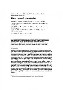
The Blas of a static pure cubic nonlinearity identified by three types of input signals . . . . . . . . . . . . . . . . . . . . . . . . . . . . . .
2.1
6
Dft power spectrum of a typical periodic Dirbs of period 𝑁 = 511 with levels ±1 . . . . . . . . . . . . . . . . . . . . . . . . . . . . . . .
16
2.2
Fibonacci implementation of Lfsr . . . . . . . . . . . . . . . . . . .
19
2.3
Illustrating and the generation of an Mlbs of period 𝑁 = 7 using a 3-bit Lfsr . . . . . . . . . . . . . . . . . . . . . . . . . . . . . . . . .
2.4
Dft power spectrum of a typical Mlbs of period 𝑁 = 511 with levels ±1 . . . . . . . . . . . . . . . . . . . . . . . . . . . . . . . . . . . . .
2.5
22
Periodic autocorrelation function of a Zoh Mlbs with bit-interval of 𝑇, period 𝑁𝑇 and levels ±1 . . . . . . . . . . . . . . . . . . . . . . .
2.6
20
22
Dft power spectrum of a typical Irbs of period 𝑁 = 510 with levels ±1 . . . . . . . . . . . . . . . . . . . . . . . . . . . . . . . . . . . . .
25
3.1
Wiener-Hammerstein system structure . . . . . . . . . . . . . . . . .
33
3.2
Wiener system structure . . . . . . . . . . . . . . . . . . . . . . . . .
35
3.3
Comparison of simulation against theory: Blas (with dc gain normalised) obtained from Gaussian and binary inputs plotted with their theoretical counterparts for a Wiener system with pure cubic nonlinearity . . . . . . . . . . . . . . . . . . . . . . . . . . . . . . . . . .
3.4
40
Comparison of simulation against theory: Blas (with dc gain normalised) obtained from Gaussian and binary inputs plotted with their theoretical counterparts for a Wiener system with pure quintic non-
3.5
linearity . . . . . . . . . . . . . . . . . . . . . . . . . . . . . . . . . .
42
Generic Volterra system structure . . . . . . . . . . . . . . . . . . . .
44
viii
3.6
Empirical (measured) Discrepancy Factors obtained from random binary sequences and Gaussian noise against theoretical Discrepancy Factors for various Wiener systems with pure cubic nonlinearity (simulation) . . . . . . . . . . . . . . . . . . . . . . . . . . . . . . . . . .
3.7
Discrepancy factor as a function of settling time of a first order linearity in a Wiener system . . . . . . . . . . . . . . . . . . . . . . . .
3.8
51
z-plane plot of the various poles configurations of the second order linearity used in Section 3.5.2 . . . . . . . . . . . . . . . . . . . . . .
3.9
50
52
Discrepancy factor as a function of the settling time of a second order linearity in a Wiener system . . . . . . . . . . . . . . . . . . . . . . .
53
3.10 Discrepancy Factor of a cubic nonlinearity 3-branch parallel Wiener system with linearities of various settling time . . . . . . . . . . . . .
54
3.11 The estimated and true Discrepancy factors in various Wiener first and second order systems . . . . . . . . . . . . . . . . . . . . . . . .
55
4.1
The robust procedure for estimating the BLA . . . . . . . . . . . . .
59
4.2
Power spectrum of a typical Dirbs of period 𝑁 = 500 with thicker circles indicating frequencies with near zero power . . . . . . . . . .
4.3
61
Performance comparison of various stochastic and invariant spectrum sequences against number of realisations of input . . . . . . . . . . .
64
4.4
Discrete Wiener system block diagram with noisy output (Oe model) 65
4.5
Performance comparison between Irbs, Mlbs and Dirbs as inputs to a Wiener system with even and odd order nonlinear distortions .
4.6
67
Performance comparison between Irbs, Mlbs and Dirbs as inputs to a Wiener system with only odd order nonlinear distortions . . . .
67
4.7
Illustration of the difference in behaviour of nonlinear distortions . .
70
4.8
Rse of the median and the mean against sample sizes in estimating Gaussian population mean. . . . . . . . . . . . . . . . . . . . . . . .
4.9
76
Log scale box-plot of absolute estimation errors of a section of a best ̂ for 𝑟 between 30 and 80 using 𝑀 = 10 linear impulse response 𝑔[𝑟] different M-sequences without output noise disturbances. . . . . . . .
79
4.10 Estimation error of the Best Linear Approximation (Bla) from outputnoise-free measurements against number of Mlbs input realisations (𝑀 ) used in averaging when using either mean or median averaging schemes. . . . . . . . . . . . . . . . . . . . . . . . . . . . . . . . . . .
80
4.11 Identification performance of various averaging schemes against Snr levels . . . . . . . . . . . . . . . . . . . . . . . . . . . . . . . . . . . .
ix
81
5.1
Designing the p.m.f. of a discrete symmetric ternary sequence . . . .
88
5.2
The p.m.f. of a symmetric ternary sequence tuned for Gaussianity .
88
5.3
Designing the p.m.f. of a discrete symmetric quaternary sequence . .
89
5.4
The p.m.f. of a symmetric quaternary sequence tuned for Gaussianity 89
5.5
Designing the p.m.f. of a discrete symmetric quinary sequence . . . .
90
5.6
The p.m.f. of a symmetric quinary sequence tuned for Gaussianity .
90
5.7
Discrepancy Factors of random ternary sequences with various zerolevel probabilities . . . . . . . . . . . . . . . . . . . . . . . . . . . . .
5.8
93
Illustration of the difference between Bla’s estimated from various multilevel uniform and optimised sequences . . . . . . . . . . . . . .
94
6.1
System schematic for the physical experiment setup in Chapter 6 . .
98
6.2
Equivalent system structure of Fig. 6.1 . . . . . . . . . . . . . . . . .
99
6.3
The use of supersampling and subsampling . . . . . . . . . . . . . . 102
6.4
Identification of the RC Linearity with op-amp based pre- and postbuffers, case 1 . . . . . . . . . . . . . . . . . . . . . . . . . . . . . . . 105
6.5
Experiment result of the identification of the Bla with Gaussian and binary inputs for an electronic Wiener system with non-ideal cubic nonlinearity and a RC linearity, case 1 . . . . . . . . . . . . . . . . . 107
6.6
Experiment result of the identification of the Bla with Gaussian and binary inputs for an electronic Wiener system with non-ideal cubic nonlinearity and a RC linearity, case 2 . . . . . . . . . . . . . . . . . 108
6.7
Experiment result of the identification of the Bla with Gaussian and binary inputs for an electronic Wiener system with non-ideal cubic nonlinearity and a RC linearity, case 3 . . . . . . . . . . . . . . . . . 109
7.1
Wiener-Hammerstein system structure . . . . . . . . . . . . . . . . . 112
7.2
Bode plot comparing the high frequency fitting of 𝐺Bla, A and 𝐺Bla, B 115
7.3
Rms errors from running optimisation (up to degree 8) on all realisable zero-pole allocations in a Wiener-Hammerstein structure. . . . . 118
7.4
Graphs of nonlinearity output 𝑤 versus input 𝑥 . . . . . . . . . . . . 119
7.5
Comparison between the gain responses of the estimated transfer functions 𝐺1 and 𝐺2 with theoretical values. . . . . . . . . . . . . . . 124
7.7
Effect of polynomial degree on simulation error . . . . . . . . . . . . 128
7.8
Effect of dual-polynomial degree on simulation error . . . . . . . . . 128
7.9
Model output and simulation error for the training data set . . . . . 129
7.10 Dft spectra of the model output (black) and simulation error (grey) for the training data set . . . . . . . . . . . . . . . . . . . . . . . . . 130 x
7.11 Static nonlinearity characteristic using coefficients from filter ID 30 . 131 8.1
Overview of the Peltier cooling system . . . . . . . . . . . . . . . . . 137
8.2
Block diagrams of Subsystems 1 and 2 . . . . . . . . . . . . . . . . . 137
8.3
Overview of the Peltier cooling system . . . . . . . . . . . . . . . . . 139
8.4
Results for the training dataset . . . . . . . . . . . . . . . . . . . . . 142
8.5
Results for the validation dataset . . . . . . . . . . . . . . . . . . . . 143
8.6
Intermediate signal for Subsystem 1 for simulation and experiment data, first and last 100 samples . . . . . . . . . . . . . . . . . . . . . 144
8.7
Intermediate signal for Subsystem 2 for simulation and experiment data . . . . . . . . . . . . . . . . . . . . . . . . . . . . . . . . . . . . 145
xi
List of Tables
2
Table of notations and for symbols and mathematics . . . . . . . . . xxv
3
Table of typesetting conventions . . . . . . . . . . . . . . . . . . . . xxvii
2.1
Xor gate truth table . . . . . . . . . . . . . . . . . . . . . . . . . . .
3.1
Moment values for zero-mean Gaussian, uniform binary and uniform ternary sequences . . . . . . . . . . . . . . . . . . . . . . . . . . . . .
5.1
21
32
Example matching of moments for Gaussianity for discrete symmetric sequences with various number of levels . . . . . . . . . . . . . . . .
87
6.1
Table of parameters and settings for the verification experiment . . . 100
7.1
Table of allocation of zeros and poles for Chapter 7 . . . . . . . . . . 117
7.2
Performance measures using the incremental nonlinear optimisation technique in terms of polynomial degree 𝑞 . . . . . . . . . . . . . . . 122
7.3
Computational time required . . . . . . . . . . . . . . . . . . . . . . 131
7.4
Comparison between several models for Chapter 7 . . . . . . . . . . 133
8.1
Comparison between several models for Chapter 8 . . . . . . . . . . 145
A.1 Table of Mlbs periodicity and set sizes for 𝑛 from 3 to 30 . . . . . . 164
xii
Acknowledgements
This thesis is dedicated to my Family, Friends and especially my Grandmother— ? A dwarf standing on the shoulder of a giant…—(Bernard of Chartres, 1159) > I very much appreciate the selfless support and kind encouragements offered by my family and friends, without whom I would not be able to overcome so many failures and relish a few triumphs; for this I am eternally indebted. I am grateful to my good friends Natalie Ellis, Alice Ng, Hui Niu, Yuan Tian, Nami Morioka, Nixon Yu, Dan Zhou; my colleagues at both the University of Warwick and the Vrije Universiteit Brussel; Mr. Ho and his family at Rugby, and many others—unsung but not forgotten. My sincerest gratitude goes to Professor Keith Godfrey and Professor Johan Schoukens, for being more than great mentors and treating me as a good friend. This endeavour would not have been possible without the technical guidance and emotional support by the two gentlemen; ‘a dwarf standing on the shoulder of two giants!’—to say otherwise is an understatement. I have to thank Keith again in particular introducing and indulging me in much British culture, from visiting cathedrals, the countryside, attending opera, ballets, orchestra and musicals to punting in horse races! I would also like to thank Dr. Ai Hui Tan for her hospitality during our visit to the Multimedia University of Malaysia and the collaboration opportunities on the benchmark studies, it was a great honour. In addition, the invaluable suggestions and encouragements offered by Professor Nigel Stocks were very much appreciated. Last but not least, many thanks to the members of the jury committee, administrative staff and lawyers, all of whom went to extraordinary lengths to make the co-tuelle arrangements and the viva for the Ph.D. possible.
xiii
List of publications arising from this research
Journal papers Tan, A. H., Wong, H. K. & Godfrey, K. R. (2012, May). Identification of a WienerHammerstein system using an incremental nonlinear optimisation technique. Control Engineering Practice, 20, 1140–1148. Wong, H. K., Schoukens, J. & Godfrey, K. R. (2012a, March). Analysis of best linear approximation of a Wiener-Hammerstein system for arbitrary amplitude distributions. IEEE Trans. Instrum. Meas. 61(3), 645–654. Wong, H. K., Schoukens, J. & Godfrey, K. R. (2013a). Design of multilevel signals for identifying the best linear approximation of nonlinear systems. IEEE Trans. Instrum. Meas. 62(2), 519–524. Wong, H. K., Schoukens, J. & Godfrey, K. R. (2013b). Structured non-linear noise behaviour and the use of median averaging in non-linear systems with msequence inputs. IET Control Theory and Applications. [Accepted for Publication]. doi:10.1049/iet-cta.2012.0622
Conference papers with peer review Wong, H. K. & Godfrey, K. R. (2010, September). A greybox approach to modelling a hyperfast switching Peltier cooling system. In Proc. UKACC International Conference on Control, 7th–10th September 2010 (pp. 1200–1205). Coventry, U.K. Wong, H. K., Schoukens, J. & Godfrey, K. R. (2012b, September). Experimental verification of best linear approximation of a Wiener system for binary excita-
xiv
tions. In Proc. UKACC International Conference on Control, 3rd–5th September 2012 (pp. 941–946). Cardiff, U.K. Wong, H. K., Schoukens, J. & Godfrey, K. R. (2012c, July). The use of binary sequences in determining the best linear approximation of nonlinear systems. In Proc. 16th IFAC Symposium on System Identification, 11th–13th July 2012 (pp. 1323–1328). Brussels, Belgium.
xv
Declarations
This thesis was submitted to the University of Warwick and Vrije Universiteit Brussel in partial fulfilment of the requirements for the Doctor of Philosophy co-tuelle agreement between the two universities. The work presented here is my own, except where specifically stated otherwise. The work was performed both in the School of Engineering at the University of Warwick under the supervision of Professor Nigel G. Stocks and Professor Emeritus Keith R. Godfrey, and in the Department of Fundamental Electricity and Instrumentation, Faculty of Engineering at the Vrije Universiteit Brussel under the supervision of Professor Johan Schoukens. The benchmark study documented in Chapter 7 was a collaboration with Dr. Tan, Ai Hui of the Multimedia University, Cyberjaya, Malaysia.
xvi
Abstract
System identification is the art of modelling of a process (physical, biological, etc.) or to predict its behaviour or output when the environment condition or parameter changes. One is modelling the input-output relationship of a system, for example, linking temperature of a greenhouse (output) to the sunlight intensity (input), power of a car engine (output) with fuel injection rate (input). In linear systems, changing an input parameter will result in a proportional increase in the system output. This is not the case in a nonlinear system. Linear system identification has been extensively studied, more so than nonlinear system identification. Since most systems are nonlinear to some extent, there is significant interest in this topic as industrial processes become more and more complex. In a linear dynamical system, knowing the impulse response function of a system will allow one to predict the output given any input. For nonlinear systems this is not the case. If advanced theory is not available, it is possible to approximate a nonlinear system by a linear one. One tool is the Best Linear Approximation (Bla), which is an impulse response function of a linear system that minimises the output differences between its nonlinear counterparts for a given class of input. The Bla is often the starting point for modelling a nonlinear system. There is extensive literature on the Bla obtained from input signals with a Gaussian probability density function (p.d.f.), but there has been very little for other kinds of inputs. A Bla estimated from Gaussian inputs is useful in decoupling the linear dynamics from the nonlinearity, and in initialisation of parameterised models. As Gaussian inputs are not always practical to be introduced as excitations, it is important to investigate the dependence of the Bla on the amplitude distribution in more detail. This thesis studies the behaviour of the Bla with regards to other types of signals, and in particular, binary sequences where a signal takes only two levels. Such an input is valuable in many practical situations, for example where the input actuator is a switch or a valve and hence can only be turned either on or off. While it is known in the literature that the Bla depends on the amplitude distribution of the input, as far as the author is aware, there is a lack of comprehensive theoretical study on this topic. In this thesis, the Blas of discrete-time time-invariant nonlinear systems are studied theoretically for white inputs with an
xvii
arbitrary amplitude distribution, including Gaussian and binary sequences. In doing so, the thesis offers answers to fundamental questions of interest to system engineers, for example: 1) How the amplitude distribution of the input and the system dynamics affect the Bla? 2) How does one quantify the difference between the Bla obtained from a Gaussian input and that obtained from an arbitrary input? 3) Is the difference (if any) negligible? 4) What can be done in terms of experiment design to minimise such difference? To answer these questions, the theoretical expressions for the Bla have been developed for both Wiener-Hammerstein (Wh) systems and the more general Volterra systems. The theory for the Wh case has been verified by simulation and physical experiments in Chapter 3 and Chapter 6 respectively. It is shown in Chapter 3 that the difference between the Gaussian and non-Gaussian Bla’s depends on the system memory as well as the higher order moments of the non-Gaussian input. To quantify this difference, a measure called the Discrepancy Factor—a measure of relative error, was developed. It has been shown that when the system memory is short, the discrepancy can be as high as 44.4%, which is not negligible. This justifies the need for a method to decrease such discrepancy. One method is to design a random multilevel sequence for Gaussianity with respect to its higher order moments, and this is discussed in Chapter 5. When estimating the Bla even in the absence of environment and measurement noise, the nonlinearity inevitably introduces nonlinear distortions—deviations from the Bla specific to the realisation of input used. This also explains why more than one realisation of input and averaging is required to obtain a good estimate of the Bla. It is observed that with a specific class of pseudorandom binary sequence (Prbs), called the maximum length binary sequence (Mlbs or the m-sequence), the nonlinear distortions appear structured in the time domain. Chapter 4 illustrates a simple and computationally inexpensive method to take advantage this structure to obtain better estimates of the Bla—by replacing mean averaging by median averaging. Lastly, Chapters 7 and 8 document two independent benchmark studies separate from the main theoretical work of the thesis. The benchmark in Chapter 7 is concerned with the modelling of an electrical Wh system proposed in a special session of the 15th International Federation of Automatic Control (Ifac) Symposium on System Identification (Sysid) 2009 (Schoukens, Suykens & Ljung, 2009). Chapter 8 is concerned with the modelling of a ‘hyperfast’ Peltier cooling system first proposed in the U.K. Automatic Control Council (Ukacc) International Conference on Control, 2010 (Control 2010).
xviii
Acronyms and Abbreviations
†
Bold page numbers point to pages in which terms are defined or explained in the text. Acronym
Abbreviation
Pages†
Adc Are Awgn Bla
Analogue-to-digital converter Asymptotic relative (statistical) efficiency Additive white Gaussian noise Best Linear Approximation
Cf Df
Crest factor Discrepancy Factor
Dft
Discrete Fourier transform
Dirbs
Discrete-interval Random Binary Sequence
Dtft Fft Fir
Discrete-time Fourier transform Fast Fourier transform Finite impulse response
98 75–77, 82 15, 58, 62, 65, 78, 82 ix, 4–9, 18, 25, 27, 28, 29–31, 33–39, 41–49, 51, 53, 55–58, 60, 63, 65, 66, 68–74, 76, 78– 80, 83, 86, 87, 91, 93– 95, 97, 99, 101, 103, 104, 106–111, 113–116, 123, 132, 145, 147–151, 165, 167, 169–172, 174, 176, 184 14, 18, 95, 96 7, 9, 47, 48–53, 55, 56, 86, 87, 91, 92, 148, 150, 151 13, 14–16, 18, 19, 21, 23, 24, 59, 69, 73, 78, 129 15, 16, 17, 32, 33, 38, 49, 61–63, 65, 66, 69, 73, 77, 78, 82–84 12, 13 20 35, 39, 65, 66, 69, 77, 109, 116, 138
xix
Acronym
Abbreviation
Pages†
Frf
Frequency response function
Ft Hlle Iir
Fourier transform Hodges-Lehmann location estimator Infinite impulse response
Irbs
Inverse-repeat Binary Sequence
Irf
Impulse response function
Lfsr Mae Miso Mlbs
Linear feedback shift registers Mean absolute error Multiple-input single-output Maximum Length Binary Sequence
Mle Mse
Maximum likelihood estimator Mean squared error
Oe p.d.f.
Output-error (model/framework) Probability density function
Pi
Periodicity-invariant (system)
Pips p.m.f. Prbs Prms rms
Performance Index for Perturbation Sequences Probability mass function Pseudorandom binary sequence Pseudorandom multilevel sequence Root mean squared
Rse Siso Snr
Relative statistical efficiency Single-input single-output Signal-to-noise ratio
4, 13, 14, 27, 39, 69, 116 4, 11, 12, 13, 106 77, 78, 82 35, 39, 77, 80, 84, 109, 116 14, 24, 63, 65, 66, 68, 83 4, 13, 14, 27, 28, 35, 38, 41, 44–46, 49, 50, 52, 53, 55, 56, 65, 69– 71, 77, 78, 80, 82, 83, 106, 109, 172, 175–177 19–21, 23, 24, 163 141, 145 135 7, 9, 18, 19–25, 32, 33, 38, 39, 60, 61, 63, 65, 66, 68, 69, 71, 72, 74, 78–80, 82–84, 99, 100, 103–105, 107, 108, 149–151, 163, 181 82 62, 66, 78, 80–83, 112, 141, 145 57, 62 xxiv, 5, 15, 17, 18, 25, 47, 75, 86 11, 12, 15, 28, 34, 35, 165 14, 95, 96 5, 25, 47, 86, 88–90, 95 18, 60, 85 25, 85 33, 100, 104, 106, 113, 114, 116, 182 74, 75, 76, 82 2, 33, 43, 136 9, 14, 16, 18, 62, 65, 77, 79, 81–83, 95, 149, 151
xx
Acronym
Abbreviation
Pages†
Wh
Wiener-Hammerstein (system)
Xor Zoh
EXclusive-OR logic gate Zero-order hold
7, 31, 33, 34, 43, 56, 86, 111, 112, 115, 116, 125, 132, 133, 147 20, 21, 24 16, 23, 53, 99, 101, 102, 112
xxi
Glossaries
Blackbox model — In system identification, the term blackbox modelling refers to the process of modelling a system through non-parametric techniques, without knowledge of physical inner workings of the system, resulting in an empirical model. 8, 112, 136, 138, 145 dc stands for direct current in electrical engineering. Regardless of the physical nature of a signal (electrical or otherwise), the terms dc offset, dc bias, dc term or dc component are all used widely in signal processing to refer to the mean value of a waveform in the time domain or the zero frequency component in the frequency domain. viii, 15, 16, 19, 23, 24, 34, 38, 39, 43, 66, 125 ELiS stands for “Estimator for Linear Systems”, a program in the Frequency Domain System Identification (Fdident) toolbox for Matlab. It implements an iterative weighted nonlinear least squares procedure that fits parametric models to non-parametric transfer characteristics of dynamical systems (Kollár, 1994). 49, 58, 91, 104, 108, 113, 114, 120, 125, 127 Empirical model — see blackbox model Galois is a program to generate pseudorandom signals including maximum-length sequences with various number of levels Barker (2008), Godfrey, Tan, Barker and Chong (2005). The signals can be designed to have desirable properties for dynamic system testing. 24, 85 Gaussianity is a qualitative measure of how close the statistical distribution of a random variable is to a true Gaussian distribution, also known as a normal distribution. xviii, 7, 9, 18, 86, 93, 96
xxii
Greybox model — In system identification, a greybox modelling approach is a mixture between whitebox and blackbox modelling. 136, see also blackbox model & whitebox model Matlab (MATrix LABoratory) is a widely used scientific numerical computation environment developed by MathWorks with its own programming language. The platform is optimised for matrix and vector based calculations and offer a wide range of tools for the manipulation, processing and visualisation of data. xxii, xxiv, 17, 24, 38, 58, 62, 63, 65, 77, 93, 98, 104, 106, 113, 116, 121, 127, 129, 137, 146, 181–183 Mechanistic model — see whitebox model Moments — see definition on p. 32. xxiii Non-parametric model is a data-driven model without a priori specification of a model structure; instead the structure is determined entirely from the data. Essentially the parameters are not fixed and typically grow in size according to the amount of data available see. 30, 39, 49, 58, 68, 91, 93, 104, 106–108, 136 Parametric model is a problem-driven model with a fixed model structure and a predetermined number of parameters. A good model can capture maximal useful information from the data used to derive it with only a few number of parameters. 49, 91, 104–108, See also non-parametric model Probability density function (p.d.f.) — In probability statistics, a p.d.f. of a continuous random variable is a density function of 𝑥 such that, when integrated over a range of 𝑥 to give the area under the curve, the area describes the relative likelihood for finding this random variable to lie within that range at any given time. The p.d.f. defines the amplitude distribution and the moments for the random variable. See also moments & probability mass function (p.m.f.) Probability mass function (p.m.f.) — In probability statistics, a p.m.f. of a discrete random variable is a discrete function of discrete variable 𝑥 that describes the relative likelihood for finding this random variable to take on a given value 𝑥 at any given time. The p.m.f. defines the distribution and the moments for
xxiii
the random variable. The p.m.f. for a discrete variable is the discrete analogue of the continuous probability density function�p.d.f.. See also moments & probability density function (p.d.f.) prs stands for “pseudorandom sequences” and is a collection of programs written for Matlab software to generate maximum-length sequences and primitive polynomials in a convenient package (Tan & Godfrey, 2002). 24, 85, 181 Simulink is a commercial tool developed by MathWorks with a tight integration with Matlab software that offers a block-oriented multi-domain programming approach to modelling, stimulating and analysing dynamic systems (Krauss, Shure & Little, 1994). 137, 138, 146, see also Matlab Uniform distribution — In probability statistics, a random variable 𝑥 with a uniform distribution has equal relative likelihood (or probability) of taking any permissible values. The uniform distribution may be discrete or continuous and is usually defined by a range, for example, 𝑎 ≤ 𝑥 ≤ 𝑏. 17, 93, See also moments, probability density function (p.d.f.) & probability mass function (p.m.f.) Whitebox model — In system identification, the term whitebox modelling refers to the process of modelling a system through first principles, laws of physics and explicit assumed relationships between the input and output through prior knowledge of the system, resulting in a mechanistic model. 8, 136, 145
xxiv
Mathematical notations and typesetting conventions
Unless otherwise specified, notations for symbols and mathematics are as follows: Table 2: Table of notations and for symbols and mathematics Symbol
Description
≈ ≡ ≜ ∀ 𝜇 𝜎 𝑒 𝑓, 𝜔 f(𝑥) f(𝑥) ↦ 𝑦 𝜋 j
... approximately equals to ... ... is a mathematical identity of ... ... by definition equals to ... ... for all ... Arithmetic mean Standard deviation Euler’s number (Napier’s constant) Frequency variables (Hz, rad s−1 ) Generic function on 𝑥 f(𝑥) is defined such that 𝑥 maps to 𝑦 Ratio of a circle’s circumference to its diameter √ Imaginary number, equals −1 Specific value 𝜃 = 𝜃′ that minimises f(𝜃) resulting in the minimised function of f(𝜃′ ) Bla (time domain) Bla (frequency domain) Sampling interval or bit-interval Continuous input signal 𝑢 at time 𝑡 Sampled input signal 𝑢 at sample 𝑘, 𝑘 counts from zero, i.e. 𝑢[0] = 𝑢(0 ≤ 𝑡 < 𝑇 )
f(𝜃′ ) = arg min f(𝜃) 𝜃
𝑔Bla (𝑡) 𝐺Bla (j𝜔) 𝑇 𝑢(𝑡) 𝑢[𝑘]
continued on next page
xxv
continued from previous page
Symbol
Description
𝑦(𝑡), 𝑦[𝑘]
Similar definitions to 𝑢(𝑡) and 𝑢[𝑘] respectively but for the output signal 𝑦 instead of 𝑢 The Dft of 𝑥 The inverse Dft of 𝑋 Big-O notation, describes the limiting behaviour of a function Gaussian (normal) distribution of mean 𝜇 and variance 𝜎2 Continuous uniform distribution between 𝑎 and 𝑏 Symmetrical discrete uniform distribution with 𝑛 levels Random variable 𝑥 follows a normal distribution 𝑥 belongs to, or is a member of, 𝒗 The factorial of 𝑥 The double factorial of 𝑥 The expected value of the random variable 𝑥 A set of 𝑥 A sequence of 𝑢 The transpose of vector 𝒗 The autocorrelation function of the signal 𝑢 The cross-correlation function between the signals 𝑦 and 𝑢 Set of natural numbers excluding zero Set of natural numbers including zero Absolute value, magnitude or cardinality (set theory) of 𝑥 𝑎 complement 𝑏 (set theory) 𝑎 is a proper subset of 𝑏 (set theory) 𝑎 is a subset of 𝑏 (set theory) The multiplicity function for multiset 𝑨 operating on element 𝑥 (set theory) s-domain operator z-domain operator Real number axis Imaginary number axis Expression 𝑥 applies given condition 𝑎 = 1 is satisfied Discrepancy Factor, see Section 3.5 Notation for Moments, see Section 3.2
ℱ{𝑥} ℱ−1 {𝑋} 𝒪 𝒩(𝜇, 𝜎2 ) 𝒰(𝑎, 𝑏) 𝒰𝑛 𝑥∼𝒩 𝑥∈𝒗 𝑥! 𝑥!! EJ𝑥K {𝑥} ⟨𝑢⟩ 𝒗T 𝑅uu 𝑅yu ℕ ℕ0 |𝑥| 𝒂\𝒃 𝒂⊂𝒃 𝒂⊆𝒃 𝟙𝑨 (𝑥) s z ℜ ℑ 𝑥|𝑎=1 𝔇 𝔐𝑛
xxvi
The conventions for typesetting are given are given in the following table: Table 3: Table of typesetting conventions Typesetting
Example
Description
De-italicised Roman Italic Uppercase italic
f, E, z−1 𝑥 𝑋
(Subscripts)
𝑘a
Bold italic lowercase Bold italic uppercase Calligraphy style
𝝃, 𝒗 𝜩, 𝑨 𝒫
Blackboard bold style Fraktur script Italicised text Slanted text
ℤ 𝔇, 𝔐 odd ID 30
Functions or domain operators Variables Complex frequency domain variables or scalar constants Descriptive subscripts are normally upright, except when the subscript itself is an index variable Sets or vectors Multisets or matrices Mathematical classes (collection of sets or multisets) or statistical distributions Number sets or speciality functions Special entities Emphasis Object labels
xxvii
xxviii
C
1
Introduction
1.1
Background of System Identification
The field of system identification and modelling is relatively modern. Before its generalisation, systems science was born out of necessity from several different fields, for example, biomedicine, neuroscience, meteorology, signal processing, communications, geology and acoustics. They all share a common goal: to create mathematical models capable of encapsulating some real processes and subsequently allow one to make prediction and, depending on application, control or influence the process to give certain desirable outcome.
1.1.1 Systems and models In the broad sense, a system is a collection of interacting entities. For example, the central nervous system is a network of interacting neurons, nerve cells as sensors and muscle cells, amongst others, as actuators. Another example is the orbits of planets around a star, which are governed by the physical law of general relativity. The former example has clear definition of inputs, measured by some sensors, and outputs, articulated by some actuators; the latter however, is less clear and depends on definition of the problem in hand. In the star system example, an astronomer may define the inputs of a star system being the masses, positions, velocities of the celestial bodies and define the output as the geometry of the orbits; understanding the model will allow the astronomer to make predictions of the output, i.e. the orbital information.
1
1.1. Background of System Identification Similarly, in system and control theory, a system is a process with single or multiple inputs directly influencing or determining the quantity of a single or some combinations of outputs. System and control engineers sought to understand the relationships between these inputs and outputs, and therefore to make predictions or devise the best way to manipulate the inputs in order to attain certain desired output behaviour. Many systems studied are dynamical—their outputs at any given time simultaneously depend on more than one past instants of inputs, outputs, or a combination of both. In other words, the outputs of the immediate future are not just determined by the inputs or outputs at this very current moment, but also the values in past moments. Exhibiting dynamics is also called having memory effects. In the frequency domain a dynamical system is characterised by having non-constant magnitude and phase frequency responses. A system without dynamics is called a static system. A model of a system is a mathematical description of the relationships governing the inputs and outputs. Such a model may contain a complete description or an approximation of the system. Unless full physical knowledge and the corresponding law of physics are well understood, it is usually not possible to devise a complete description. To be able to understand the relationship between the inputs and outputs, it is necessarily to apply techniques from the disciplines of system identification and modelling. System identification is the art of extracting information and gathering data efficiently and accurately from the system in question with certain user-specified goals. Sometimes it is possible to take control of an input, which simplifies the process. In such cases, the choice of the types and properties of input signals is important to the quality of information extracted. With data gathered, one can then start building models of the system. System modelling, on the other hand, is the art of choosing, developing and validating models that give the most accurate and precise description of the real system based on the finite measurement data obtained from system identification. A good model allows one to predict the output or outputs of a system given some arbitrary inputs, or at the very least, normal operating inputs expected for the real operation of the system. Once a model has been derived and validated, the foundation is set for control engineers to devise optimised control schemes to influence a system to achieve certain desired behaviour. In this thesis, for simplicity, only dynamical systems with a single input and a single output are considered, these systems are referred to as single-input singleoutput (Siso) systems. The systems considered are also time-invariant. This is to say, the system dynamics, structure and behavior remain unchanged with time so
2
1.1. Background of System Identification that under the same input and given the same initial conditions, the system always generates the same output.
1.1.2 Linear and nonlinear systems Linear models are well documented and commonly used, even when the underlying system is nonlinear (Ljung, 1999, tbl. 4.1). The concept of linearisation and proportionality is well known and used in a wide range of fields. Some relationships in nature are predominantly linear, some are very nonlinear and there are those in between. All ‘linear’ systems are nonlinear to a certain extent—there are no true linear relationships, as ultimately the linearity breaks down at some extreme points due to changing law of physics or when external factors are introduced and starting to dominate. Even with moderately nonlinear systems, linear models of sufficient quality can be obtained given a small enough input domain or operation range. Mathematicians, scientists and engineers prefer to apply linear approximations because their simplicity opens the door for closed-form algebraic study and allows models to be devised with minimal effort and cost. Definition A nonlinear system is a system where the input-output relationship(s) does not obey the principle of superposition. An example of a nonlinear system is the human auditory system—doubling the power output of a loudspeaker does not double the perceived loudness. It also has dynamics—different loudness is also perceived for tones with different frequencies. Note that in this thesis, the term nonlinear system is used for a dynamical nonlinear system while the term static nonlinearity is used to refer a static nonlinear entity.
1.1.3 Impulse and impulse response Before the existence of modern system identification techniques, a frequently used excitation signal called an impulse function (more formally the Dirac delta function) has been used throughout human history, even before its mathematical understanding was developed. Since the ancient times, people have found that one can examine the quality, material, geometry or mass of an object by striking it with a short-lasting impact. For example, knocking on a hollow object produces a distinctively different sound than that produced by knocking on a solid object. By listening to the knock, one performs an ‘identification’ with one’s ears and brain—together make a surprisingly good biological audio frequency spectrum analyser! Many musical instruments also rely on impulses. For instance, pianists play sound by hitting keys, which causes 3
1.1. Background of System Identification tensioned wires in the piano to be struck by hammers. Each key corresponds to a different wire that was taut with a specifically tuned tension force (or made with an entirely different metal), in order to have its resonant frequency corresponding to a particular musical note. The strike of the hammer is effectively an impulse that causes the struck wire to vibrate and resonate at its natural frequency. This vibration interacts with the sound board of the piano and the surrounding air to produce the musical note as a perceivable sound. An example of successful application of impulses in a system identification problem is in the analysis of the acoustics of a concert hall though gunshots and even balloon bursts (Sumarac-Pavlovic, Mijic & Kurtovic, 2008). With an impulse as excitation, it is possible to extract information of the dynamics from a system. The response as a function of time of a linear dynamical time-invariant system to an applied impulse is called the impulse response function (Irf), and is sufficient to describe the dynamics (but not the inner-structure) of a linear time-invariant dynamical system. Knowing the Irf allows one to predict the output of the system under any arbitrary inputs (not outside operating ranges that may induce nonlinear effects). Because of this, the objective of many system identification exercises is to obtain the Irf. The frequency response function (Frf) is the analogue of the Irf in the frequency domain. Through the use of Fourier transform (Ft) there is a one-to-one mapping between the frequency domain and the time domain (see Section 2.2). For nonlinear systems, the closest analogue of an Irf is the Volterra kernel (Volterra, 1930/2005), akin to a multidimensional Irf. This will be discussed in more detail in Section 3.4. However, it is possible to devise an Irf to represent a linear model that behaves, as close as possible, to a nonlinear system. One such tool is the Best Linear Approximation (Bla), introduced in the next section and discussed in more technical detail in Section 3.1.
1.1.4 The Best Linear Approximation (B) To devise a model to fit the relationship of some data variates, firstly one has to define a measure of error between the model prediction and the true measured data, called the cost function. A popular choice is the least squares cost, where the total error is defined as the total squared differences between the model prediction and the true measurement. A model where this total error is minimised is called the least squares model. For example, in statistics, the ordinary least squares linear regression is a type of least squares model.
4
1.1. Background of System Identification In dynamical systems, the least squares linear time-invariant model of a nonlinear time-invariant system is called the Best Linear Approximation (Bla). It was founded on the basis of the Bussgang theorem (Bussgang, 1952) and it has several important properties under the influence of input signals having Gaussian p.d.f’s.: firstly, the transfer characteristics of a block-structured nonlinear system is the combined dynamics multiplied by certain constant factor depending on the nonlinearity (for example, see Section 3.3); and secondly, the Bla of a static nonlinearity is static. In this thesis, for convenience, the Bla obtained from signals bearing a Gaussian p.d.f. (or p.m.f. for discrete sequences) shall be called the Gaussian Bla. However, the aforementioned properties do not apply if the inputs to the nonlinear system do not have a Gaussian distribution. Example 1.1 of Enqvist (2005) shows that the Bla of a static nonlinearity for non-Gaussian inputs is not necessarily static. Further, example 1.2 from the same source shows that the Bla can be different for two inputs despite sharing an equal colour (or power spectrum). A motivation example illustrating the dependence of the Bla on the amplitude distribution of the input signals is given as follows: Example Consider a simple pure cubic nonlinearity such that the output 𝑦 is related to the input 𝑢 by 𝑦 = 𝑢3 , and hence there are no dynamics. Three types of zero-mean inputs: Gaussian, symmetrical (about zero) binary (2-level) sequences and symmetrical ternary (3-level) sequences are used to identify the Bla of the cubic nonlinearity. The binary and ternary sequences have their levels uniformly distributed, i.e. all their levels have equal probability of appearance, the value of which is 1/2 for the binary levels and 1/3 for the ternary levels. The power of all three sequences is normalised to unity. As a result, the variance of the Gaussian input is also unity. For the other two sequences, the power normalisation combined with the symmetry dictate that the binary sequence to comprise levels +1 and −1 √ √ and the ternary sequence to comprise levels of + 1.5, 0 and − 1.5 (see methods in Chapter 5 for the derivation). The results are shown in Fig. 1.1. It can be seen that the Blas are indeed different for all three types of inputs. This is understandable as the Blas are optimised to approximate the nonlinear cubic relationship to their best ability (in terms of least squared errors) within the range of input amplitudes of their corresponding input signal. This means that for the binary case, the Bla is exactly described by 𝑦 = 𝑢, as the error between 𝑦 = 𝑢 and 𝑦 = 𝑢3 is exactly zero given input levels 𝑢 ∈ {+1, −1}. For the Gaussian case the Bla is 𝑦 = 3𝑢 while for the ternary case the Bla is 𝑦 = 1.5𝑢. The theoretical steps to derive these Blas shall not be discussed here as the theory is not introduced until Chapter 3. Nonetheless, note that the coefficient of 𝑢 of each Bla in this example is directly 5
1.2. Thesis outline equal to the 4th order moments of the corresponding input. The concept of moments will be introduced in Section 3.2 and within which, Table 3.1 contains the central moments for the three types of sequences used in this example. 8 6 4
y
2 0 −2 y = u3 Gaussian BLA Binary BLA Ternary BLA
−4 −6 −8 −2
−1.5
−1
−0.5
0 u
0.5
1
1.5
2
Figure 1.1: The Blas of a static pure cubic nonlinearity identified by three types of input signals
As mentioned before, Gaussian Blas have desirable and well known properties. However, in some systems, one cannot expect the inputs to have a Gaussian distribution—the flow rate of a fluid controlled by an on-off valve for example, is more binary in nature; this sets the motivation of the thesis. Questions arise, for example, what happens if a binary excitation is used instead of a Gaussian noise excitation? Will the results significantly change, or will the differences be sufficiently small that, for practical purposes, they can be ignored? Is it possible to quantify the differences between non-Gaussian and Gaussian excitations on the basis of the non-Gaussian measurement results? These questions will be addressed in Chapter 3.
1.2
Thesis outline
This thesis is split into two parts containing nine chapters in total. The first six chapters revolve around the main topic on the theory of the non-Gaussian Bla.
6
1.2. Thesis outline Chapters 7 and 8 are both standalone chapters each documenting a benchmark study. The last chapter contains general conclusions, a discussion on future work and a summary of contributions. Details of each chapter in this thesis are listed as follows: Chapter 2 introduces the various periodic input sequences used throughout this thesis with discussions on their properties and how they are generated. The first part of Chapter 3 gives a formal definition of the Bla and shows that it is possible to derive closed-form expressions for the Blas obtained from signals with arbitrary amplitude distributions for any time-invariant discrete-time systems; within which two types of systems are shown: firstly the block-structured Wiener-Hammerstein (Wh) system in Section 3.3 and secondly for the more general Volterra systems in Section 3.4. The second part of Chapter 3 introduces a measure to quantify the difference called the Discrepancy Factor (Df) in Section 3.5. This answers the question on how much the Bla deviates from the Gaussian obtained counterpart and it is shown that systems with shorter memory, in general, have higher Dfs. The first part of Chapter 4 introduces a method for identifying the Bla and discusses the behaviour of exogenous environment (and measurement) noise and nonlinear distortions arising from the nonlinearities, with respect to different available input sequences introduced in Section 2.3. The second part from Section 4.5 onwards documents a method to improve the estimates of the Bla through using alternative averaging schemes rather than the conventional mean function, by using a special property of Maximum Length Binary Sequence (Mlbs) inputs resulting in structured nonlinear distortions. The results show such a method is simple to apply and effective in low exogenous noise scenario. Chapter 5 illustrates a method to design discrete-interval random multilevel sequences for Gaussianity. Gaussian Bla has well documented properties, one of which is the ability to decouple the dynamics from the static nonlinear contributions. Some problems prohibit the use of continuous amplitude levels, examples of which are given in the beginning of the chapter. In such situations, optimising multilevel sequences for Gaussianity is one method to obtain an unbiased Gaussian Bla. Chapter 6 details an experiment based on an electrical circuit in a Wiener system configuration conducted to verify the discrete-time Bla theory developed in Chapter 3, in which only simulated experiment was conducted. The experiment results successfully verified the theory in a laboratory setting. Chapter 7 proposes a solution to the benchmark problem with a WienerHammerstein electrical system published in Schoukens, Suykens and Ljung (2009).
7
1.3. Contributions The content of this chapter is based on Tan, Wong and Godfrey (2012). The chapter shows a utilisation of one property of the Gaussian Bla—the Bla is proportional to the combined linear dynamics of the system. This allows a brute-force exhaustive search of all poles and zero combinations resulting in two physically realisable filters for the first and second linearities of a Wiener-Hammerstein system. The iterative algorithm proposed also models the static nonlinearity using a polynomial or a piecewise polynomial function. The parameters are tuned in multiple stages, first for linearity assignment, then to nonlinearity, to minimise the number of parameters the optimisation algorithm has to tackle at any stage. The polynomial degrees are increased one degree at a time to minimise the chance of the optimisation being stuck in a local minimum. Chapter 8 documents a modelling exercise on a ‘hyperfast’ Peltier cooling system assembly (Cham, Tan & Tan, 2010). The solution encompasses a mixture of blackbox and whitebox modelling approaches, incorporating as much physical and structural knowledge of the system as possible and without relying on numerical non-parametric optimisation methods. The solution shows that even a simple, naïve approach that does not use established sophisticated system identification methods, can yield models with acceptable performance given enough prior physical knowledge. This piece of work was based on Wong and Godfrey (2010).
1.3
Contributions
Much of the research documented in this thesis has previously been published in journal or conference publications; a list of which is available on p. xiv. Unless otherwise specified or referenced, all the work are performed by the author under the guidance of the supervisors named on p. ii with the exception of Chapter 7 which was part of a collaboration (see p. xvi). Major contributions arising from the research work performed over the course of this Ph.D. degree are highlighted in this section as follows: The objective of this thesis is mainly concerned with the use of non-Gaussian signal in identifying the Bla of the system. While the dependence of the Bla on the input amplitude distribution is well known in the literature, the work in Chapter 3, first published in Wong, Schoukens and Godfrey (2012a), tackles some questions relevant to the system identification community. To the best of the author’s knowledge, the effect of non-Gaussianity of inputs to the Bla of a time-invariant discrete-time nonlinear system has not been investigated in detail, and this thesis is able to provide closed-form algebraic expressions for the Bla of generalised discrete-time Volterra
8
1.3. Contributions systems with arbitrary input distributions. This answers the question made in the beginning of the chapter: ‘What happens if a binary excitation is used instead of a Gaussian noise excitation?’. Another question is: ‘Will the results significantly change, or will the differences be sufficiently small that, for practical purposes, they can be ignored?’. The simulation experiments performed for a Wiener system with a) cubic (Section 3.3.1) and b) quintic (Section 3.3.2) nonlinearity have shown that the Gaussian Bla and the Bla obtained from other input signals can have a significant difference between them. Finally, to answer: ‘Is it possible to quantify the differences between non-Gaussian and Gaussian excitations on the basis of the nonGaussian measurement results?’, a measure called the Discrepancy Factor (Df) was developed in Section 3.5 to quantify the difference. The first part of Chapter 4 discusses the behaviour of noise and nonlinear distortions and how it affects the choice of input signal. This piece of work was also published in Wong, Schoukens and Godfrey (2012c). In the second part, significant improvement to the quality of estimate of the Bla of a nonlinear system can be made when the input sequences used were Maximum Length Binary Sequences (Mlbs’s), giving rise to nonlinear distortions having a certain structure unique to Mlbs’s. While this structured behaviour is known in the literature, see for example, Godfrey and Moore (1974), Vanderkooy (1994), the structured nonlinear noise has been treated as a negative aspect rather than an opportunity. In this thesis, it was found that the use of alternative averaging schemes rather than the traditional mean-based averaging can offer significant improvement in the Bla estimate under moderate to high signal-to-noise ratio (Snr) due to the structured nonlinear distortions. The findings were submitted as Wong, Schoukens and Godfrey (2013b), which has been accepted for publication. Another notable contribution involves the physical experiment performed to verify the theory developed in Chapter 3, documented in Chapter 6 of this thesis and published in Wong, Schoukens and Godfrey (2012b). Here the experiment showed good agreement between the theory and practice. Furthermore, noting the dependence of the Bla on Gaussianity of the input signal, the author investigated the merits in designing discrete-time discrete-level sequences up to 5 levels (quinary) to match the higher order statistics to a discretetime Gaussian sequence. Chapter 5 has shown that it is possible to, depending on the degree of nonlinearity, minimise or completely eliminate the bias of the estimated Bla with respect to the Gaussian Bla. This piece of research was also published to Wong, Schoukens and Godfrey (2013a) and was presented at the 31st Benelux Meeting on Systems and Control, held on the 27th –29th , March, 2012 in Heijen, the
9
1.3. Contributions Netherlands. Lastly, the benchmark Chapters of 7 and 8 document solutions to benchmark problems previously proposed in two separate conferences. The benchmark studies provided valuable training opportunities for the author in system identification.
10
C
2
Periodic Input Sequences
eriodic sequences are widely used in system identification. They offer several
P
advantages over aperiodic sequences in, for instance, eliminating spectral leakage
(see Section 2.2), the ability to perform inter-period averaging to drive down the effect of exogenous environment noise (see Section 4.2) and allowing the user to compare the level of nonlinear distortions to that of noise (Pintelon & Schoukens, 2012). Several types of periodic input sequences used throughout this thesis are described in this chapter. Before these sequences are introduced in Section 2.3, two concepts first explained: periodicity-invariant (Pi) property in Section 2.1 and the various Fourier transforms (Fts) in Section 2.2.
2.1
Periodicity-invariance (Pi)
Definition A nonlinear system is designated as periodicity-invariant�Pi when excited by any periodic input 𝑢 with period 𝑁; the noise-free output 𝑦 would always share the same period 𝑁. This is the case if the spectral harmonic frequencies of the discrete output spectrum are all divisible (in whole) by the fundamental frequency of the periodic input. For linear dynamical systems, the Pi property always hold true, as the existence of transfer functions dictates that the output frequency grid to be equal to that of the input. In some literature, e.g. Marconato, Van Mulders, Pintelon, Rolain and Schoukens (2010), Pi systems are denoted period-in-same-period-out (Pispo) systems.
11
2.2. Fourier transformations and periodicity In this thesis, the focus is on periodic sequences due to several advantages highlighted in the next section, and as such all nonlinear systems considered are restricted to Pi systems.
2.2
Fourier transformations and periodicity
A signal is a carrier of information and it may take different physical forms: electrical such as voltage values; or mechanical such as the angle of a valve controlling the flow rate of some fluid. A signal can also be either continuous (in amplitude), an analogue signal; or discrete, a digital signal. Throughout this thesis, the term sequence is used only to denote digital signals. The spectral density of an infinitely long aperiodic continuous time signal not described by a finite sum of sinusoids is a continuous function of frequency, and is obtained by the continuous Fourier transform (Ft). The Nyquist-Shannon sampling theorem states that the sampling frequency should be more than twice as high as the highest frequency content of a band-limited signal to be able to reconstruct the original signal with no loss of information. When an infinitely long analogue signal is sampled at fixed time intervals to create a sequence, with sampling frequency 𝑓s (or sampling interval 𝑇 = 1/𝑓s ) chosen to obey the Nyquist-Shannon sampling theorem, the spectral density is given by the discrete-time Fourier transform (Dtft), defined for a sampled input 𝑥[𝑘] as: ∞
𝑋Dtft (𝑒j𝜔 ) = ∑ 𝑥[𝑘]𝑒−j𝜔𝑘
(2.1)
𝑘=−∞
where 𝑘 = 𝑛/𝑓s for all integer 𝑛 ∈ ℤ. With respect to this equation, the Dtft manifests repeated spectral ‘copies’ of the Ft of the continuous signal, with each copy centred at frequencies 𝑛𝑓s ∀𝑛 ∈ ℤ. If one normalises the angular frequency variable from 𝜔 = 2𝜋𝑓, with units of radian per second, to 𝜔 ⟶ 2𝜋𝑓/𝑓s = 2𝜋𝑓 𝑇, the periodicity of the 𝑋Dtft over frequency then becomes exactly 1. Provided the Nyquist-Shannon theorem is satisfied, the overlapping or spectral aliasing between different copies is nil. In practice many signals are not truly band-limited and hence there is always a certain amount of aliasing; but with careful measurement strategy, e.g. with proper use of anti-aliasing filter, this can be minimised. In both cases the spectral density is a density function since the distribution is continuous over frequency and has dimension Hz−1 . In reality, it is a necessity to perform measurement in finite time. When a truncation of an infinite signal or sequence is made to create a finite data record,
12
2.3. Periodic input sequences i.e. applying a rectangular time-window to obtain a snapshot, the record is assumed periodic when transferred to the frequency domain through the discrete Fourier transform (Dft), defined as: 𝑁−1
𝑋Dft (𝑘) = ∑ 𝑥[𝑛]𝑒−j2𝜋𝑘𝑛/𝑁
(2.2)
𝑛=0
for 𝑘 = 0, 1, ... , 𝑁 − 1. The principal difference between Dft and Ft/Dtft is that the Dft 𝑋Dft (𝑘) is always discrete in frequency. By imposing the input 𝑥 to have a periodicity of 𝑁, 𝑋Dft (𝑘) in essence becomes the 𝑁-point sampled version of the 𝑋Dtft around the unit circle in the complex plane, at the points 𝜔𝑘 = (2𝜋𝑘/𝑁). This results in a power spectrum containing a discrete number of frequency lines, rather than power spectral density. Power spectrum is dimensionless in terms of time (i.e. involves only the unit of measurement, but not Hertz). If the original signal is aperiodic, the Dft is only an approximation due to spectral leakage caused by truncation. Different windowing functions such as the Hanning (named after Austrian meteorologist Julius von Hann) window are traditionally used instead of the rectangular window (simple truncation) to improve the estimate (Blackman & Tukey, 2012). In the case of periodic signals, the Poisson summation formula (developed by French mathematician Siméon Denis Poisson) also shows that the periodic summation of a function in the time domain is described completely by discrete samples of its Fourier transform. The converse is also true—the periodic summation of a function in the frequency domain is described completely by discrete samples of the original function in the time domain (Pinsky, 2002). Hence, in such cases, both the time domain and frequency domain functions are periodic and contain an equivalent description of one another. In addition to linking a signal or sequence to its power spectrum, Fts are also used for transforming an impulse response function (Irf) (see Section 1.1.3) in the time domain to its frequency response function (Frf) frequency domain counterpart. If the Dft is used, the resulting Frf 𝐺(z) is valid for predicting the output of a discrete-time dynamical system 𝑌(z) = 𝐺(z)𝑈(z) when subjected to discrete-interval periodic input excitation 𝑈(z), in steady-state.
2.3
Periodic input sequences
System identification is concerned with the extraction of dynamics from a system through some form of measurements on the inputs and outputs. In some situations, it is not possible to design an excitation signal or even apply one to a system depend-
13
2.3. Periodic input sequences ing on its nature. For example, one only has a limited control on the concentration of a drug in a patient. In many problems however, the input signal is only restricted by the maximum amplitude limits of an actuator or by the maximum power a system can handle without its integrity being compromised. There are two important properties that make an input signal viable for system identification for linear systems. Firstly, a signal must be ‘persistently exciting’ (see Shimkin & Feuer, 1987; Söderström & Stoica, 1989, def. 5.1) such that the Irf or Frf can be extracted through mathematical operations; and secondly, a signal should contain maximal spectral content (or power) in the frequency band of interest to maximise the signal-to-noise ratio (Snr) of the estimates, and with enough frequency resolution to discern between features of interest, for example, sharp resonances. The impulse, introduced in Section 1.1.3, is a persistently exciting white signal that contains equal energy content in all frequencies. Impulses however, have a major disadvantage—being a signal that lasts only a very short period of time, the energy transmitted to the system-under-test is limited. When the environment has significant background noise, the impulse response can be overwhelmed and buried by noise, leading to a poor quality measurement. There are many metrics to quantify the suitability of signals for noisy linear system identification, two of which are crest factor (Cf) and Performance Index for Perturbation Sequences (Pips) (see Schoukens, Pintelon, van der Ouderaa & Renneboog, 1988; Godfrey, Barker & Tucker, 1999; Pintelon & Schoukens, 2012, and also Section 5.4). For nonlinear system identification, it can be useful to intentionally suppress spectral lines to gauge the degree of nonlinearity distortions or to minimise them; one example is shown by using the Inverse-repeat Binary Sequence (Irbs) with odd-harmonics suppressed in Section 4.4. Rather than concentrating the energy in one burst in a short time window, many excitation signals continuously transfer energy into the system, limited only by actuator amplitude or the system energy balance (to avoid overheating, breakdown, etc.). Such signals are now a preference over impulses due to the higher Snr achievable. Thanks to the development of electronics such as digital-to-analogue converters, computers, signal processing algorithms, efficient implementation of Fourier transform algorithms such as the fast Fourier Transform (Fft), more complex signals can be precisely and reliably generated, and measurement results can be interpreted with sufficient computing power. In this section, several types of sequences mentioned in this thesis are introduced. The use of periodic sequences has an advantage in that the Dft is completely immune to spectral leakage if the sequence was sampled at precisely the right time
14
2.3. Periodic input sequences points, (i.e. at the correct frequency) to create records of a complete period. Another advantage is that transient effects are easy to minimise or eliminate during measurement. Because of these advantages, periodic sequences should be used as excitations for system identification of Pi systems wherever possible. All of the discrete-time excitations considered in this thesis are periodic. Zero-mean or near zero-mean sequences are used and therefore the dc level (zeroth frequency) is either exactly or approximately zero. Note that in this thesis, where a periodic discrete-interval sequence is said to have a period of 𝑁, the unit is in samples. This gives a period in seconds of 𝑁𝑇, where 𝑇 is the bit-interval of the signal generator in seconds. For the specification of periods hereinafter, the units may be omitted; 𝑁𝑇 seconds and 𝑁 samples are used interchangeably.
2.3.1 White Gaussian noise Aperiodic white Gaussian noise is a typical signal used in modelling environment and measurement noise, in which case the acronym Awgn for additive white Gaussian noise, is often used in the literature. The term ‘white’ refers to the fact that the power spectral density of the signal has a flat expected power in all frequencies within a certain frequency band of interest—an infinite bandwidth signal does not exist in reality, as such a signal would have infinite energy due to the infinite spectral content. Nevertheless such a mathematical model usually suffices to model a broadband (wide spectrum) noise that is white as far as the band of frequency of interest is concerned. The term Gaussian refers to the amplitude distribution or the probability density functions�p.d.f’s. of finding the signal level at any given time as being normally distributed. Periodic white Gaussian noise may be utilised as excitation signals for system identification. A discrete-interval white Gaussian noise sequence can be obtained when the noise is sampled at fixed time intervals. When the sequence is truncated into multiple records and each of which is made periodic, the magnitudes of their Dft spectra are stochastic. The Dft power spectrum of each record is not strictly white, but after sufficient averaging of many records, the ensemble power spectrum tends to a white spectrum (see Section 4.3).
2.3.2 Discrete-Interval Random Binary Sequences (D's) A Discrete-interval Random Binary Sequence (Dirbs) is a discrete-interval sequence of values taking only two levels, a high or a low, with equal probabilities—see, for
15
2.3. Periodic input sequences example, Godfrey (1980). If the high and low levels are chosen to be +𝑉 and −𝑉 respectively, the expected value of such a sequence is zero. Dirbs’s are aperiodic, and as their length approaches infinity, their autocorrelation functions are asymptotically equal to: 𝑅uu [𝑘] = {
𝑉2 0
𝑘=0 𝑘≠0
(2.3)
Through truncation and splitting into records of length 𝑁, periodic Dirbs’s can be obtained, reaping the benefits associated with periodic sequences in terms of eliminating spectral leakage and allowing for inter-period averaging to reduce the output noise variance. They are not as useful for linear system identification as other sequences because of the need either to use a very large value of 𝑁 in order for their off-peak autocorrelation function to be small, or equivalently, by using a large number 𝑀 of different segment realisations with a much smaller value of 𝑁 and then averaging the results; in either case, a relatively long experimentation time is needed. If 𝑀 is not large, then it is possible for the Dft at some of the harmonics to be relatively small, resulting in a low Snr at those frequencies—this is discussed in more detail in Section 4.3. 0
Power (dB)
−10 −20 10 log
−30 −40 −50
0
20
40
60 80 Frequency line
230
250
Figure 2.1: Dft power spectrum of a typical periodic Dirbs of period 𝑁 = 511 with levels ±1 Periodic Dirbs’s have similar Dft spectral properties as periodic white Gaussian noise sequences introduced in the previous section. The power spectrum on a decibel (dB) scale of a typical Dirbs of length 𝑁 = 511 is presented in Fig. 2.1. When taken as a whole, the Dft power spectra for a family of zero-mean zero-order hold (Zoh) Dirbs’s with power normalised to unity and period 𝑁 have zero power in dc (zero frequency or the constant term); the remaining power (of unity) is evenly 16
2.3. Periodic input sequences distributed between the remaining 𝑁 − 1 spectral lines. In decibel scale this gives 1 across the non-zero frequency lines and an ‘expected value’ of power of 10 log10 𝑁−1
this is marked in Fig. 2.1 by a dashed line. Note that the 𝑦-axis is on a decibel scale, hence the dashed line does not look like a ‘line of best fit’. Lastly, because of the stochastic nature, each different realisation of Dirbs has a different power spectrum as seen in the figure; this is in contrast to random-phased multisines (user-defined) and pseudo random sequences, described in later sections.
2.3.3 Random-phased multisines Periodic multisines are widely used in both linear and nonlinear system identification. Their periodic nature avoids the need to deal with leakage effects. A multisine is a periodic analogue signal constructed by summing a finite number of sine waves with a certain frequency range and phase relationships between them. A multisine 𝑥(𝑡) with a linearly spaced frequency grid is defined as: 𝐹
𝑥(𝑡) = ∑ 𝐴(𝑘) sin(2𝜋𝑘𝑡𝑇s /𝑇N + 𝜙(𝑘))
(2.4)
𝑘=1
where 𝑇s is a sampling period of the signal generator, 𝑇N is the period of the multisine, 𝐹 is the maximum number of allowed frequencies, 𝐴(𝑘) and 𝜙(𝑘) are the amplitude and phase for each harmonic 𝑘 (Schoukens, Pintelon & Rolain, 2012, p. 38). A continuous multisine may be sampled to obtain a digital multisine signal. The user may choose both the power spectrum and the phases of the complex frequency spectrum. A common design choice is to excite a range of frequency band with fixed power and zero power in other frequencies. Appendix B.2 shows the implementation of a Matlab routine that generates random-phased multisines with flat power spectra. When the phase of the sine waves at the excited frequencies are designed to follow a continuous uniform distribution such that ⟨𝜙⟩ ∼ 𝒰(−𝜋, 𝜋) (between −𝜋 and 𝜋 radians), random-phased multisines are obtained. This is not the only way to design the phases; for example, Schroeder-phased multisines have a special phase structure, resulting in a signal resembling somewhat a chirp1 (Schroeder, 1970; Boyd, 1986). This thesis focuses on random-phased multisines because of several desirable properties in nonlinear system identification: firstly, the Gaussian p.d.f. of the resulting signal in the time domain; secondly, the ability to generate many independent realisations of them with similar properties and thirdly, their 1 A chirp signal is a sine wave with its frequency component continuously and monotonically increasing (or decreasing) over time
17
2.3. Periodic input sequences similarity to Gaussian noise in the time domain while having an invariant and userdefined Dft power spectrum. The asymptotic Gaussian p.d.f. property is especially important to the bias-free identification of the Best Linear Approximation (Bla) (see Chapter 3). A random-phased multisine has a relatively high Cf (Schoukens, Pintelon, van der Ouderaa & Renneboog, 1988), compared to, say, a binary sequence. Various literature in the past (see for example, Schroeder, 1970; van der Ouderaa, Schoukens & Renneboog, 1988; Guillaume, Schoukens, Pintelon & Kollár, 1991) has tackled this problem by optimising the phase through various methods to produce a signal with lower Cf, meaning that energy content of the resulting signal is more efficiently packed in a tight amplitude profile. Since many actuators are limited by their output amplitude, a high energy content is required for a high Snr. Doing so however inevitably changes the amplitude distribution of the signal, making the resulting multisine signal no longer Gaussian. In this thesis, the Gaussianity of a signal plays an important aspect and hence the Cfs are not optimised. A band-limited multisine may be sampled to give a discrete multisine sequence. In subsequent usage of the term random-phased multisine sequence or simply multisines, the thesis refers to a white discrete Riemann equivalent (see Schoukens, Dobrowiecki, Rolain & Pintelon, 2009; Schoukens, Lataire, Pintelon, Vandersteen & Dobrowiecki, 2009) random-phased multisine with all harmonics up to the Nyquist frequency excited with equal power, essentially creating a white Dft spectrum. The spectral whiteness is necessary for maintaining a fair comparison with the m-sequences detailed in the next section.
2.3.4 Maximum Length Binary Sequences (M's) Maximum Length Binary Sequences (Mlbs’s) or m-sequences are discrete-time signals belonging to a class of pseudorandom binary sequences (Prbs’s) (Godfrey, 1993; Godfrey, Tan et al., 2005). These are sequences generated with linear autorecursive relations designed to achieve maximum periodicity (Zierler, 1959; Barker, 1967; Golomb, 1981). Some use the term Prbs to refer to Mlbs but it is important to note there are other binary sequences that fall under the umbrella of Prbs, for example, quadratic residue binary sequences, Hall binary sequences and twin-prime binary sequences (Godfrey, Tan et al., 2005; Barker, 2008). The term ‘pseudorandom’ stems from the fact that these sequences, while having properties of randomness, are actually deterministic. This deterministic nature means that there are a limited number of sequences given any period (or length) 𝑁 and each one of them is unique. Two of the most important properties 18
2.3. Periodic input sequences of Mlbs’s are their perfectly flat Dft power spectra (except dc) and the shift-andadd(multiply) property (see p. 24). The flat power spectra make Mlbs’s versatile in system identification and the shift-and-add property has implications in nonlinear distortions (see Chapter 4). More properties of Mlbs’s are listed on p. 23. Due to their favourable cross-correlation characteristics, deterministic nature and ease of generation through simple shift register circuitry (Golomb, 1981; Norton, 1986/2009; Godfrey, 1993), m-sequences have been used extensively from communications (Simon, Omura, Scholtz & Levitt, 1994) to system identification in a wide range of fields including acoustical (Borish & Angell, 1983), chemical (Amrani, Dowdeswell, Payne & Persaud, 1998), industrial (Godfrey & Moore, 1974; Vilkko & Roinila, 2008) and physiological (Marmarelis, 2004) systems. Mlbs’s have unique properties when applied to nonlinear system identification, the shiftand-add(multiply) property for example, allows better than normal rejection of nonlinear distortions, specifics of which will be discussed in Section 4.5.1. Another example is that these sequences are especially suitable when estimating higher-order Volterra kernels (see Section 3.4)—normally a time-consuming and inaccurate procedure (Sutter, 1987, 1992; Reed & Hawksford, 1996). Galois field mathematics
𝑔1
𝑔0 ≡ 1
⋯.
𝑔 .2
+
𝑔 𝑛−1 𝑔𝑛 ≡ 1
Figure 2.2: Fibonacci implementation of Lfsr Mlbs’s can be generated from electronic linear feedback shift registers (Lfsr) with special feedback topology, which gives the maximum periodic length (period) attainable by traversing all binary 𝑛 ≥ 3-bit patterns within the Lfsr except one (all zeros) of 𝑁 = 2𝑛 − 1. Any Lfsr can be represented by a generator polynomial 𝐺(𝑥) such that: 𝐺(𝑥) = 𝑔0 ⊕ 𝑔1 𝑥1 ⊕ 𝑔2 𝑥2 ⊕ ... ⊕ 𝑔𝑛−1 𝑥𝑛−1 ⊕ 𝑔𝑛 𝑥𝑛 (mod 2)
(2.5)
where 𝑔𝑛 represents the feedback tap configurations and numerically equal to 1 when connected and 0 otherwise. For practical reasons, 𝑔0 and 𝑔𝑛 must be set to 1, i.e. connected, see Fig. 2.2. The 𝐺(𝑥) is performed in modulo-2 mathematics for binary sequences and obey modulo-2 addition (denoted by ⊕) and modulo-2 multiplication 19
2.3. Periodic input sequences (for the raised powers) operations. Modulo-2 addition is handled electronically by eXclusive-OR logic gates (Xors). A sequence with maximum period 𝑁 = 2𝑛 − 1 permitted by the number of Lfsr bits 𝑛 is generated only when the feedback topology can be described by a primitive polynomial. Definition 𝐺(𝑥) is a primitive polynomial if it cannot be factorised into any polynomials of a lesser degree, and it is a factor of the polynomial 𝑥𝑁 + 1 (mod 2) where 𝑁 = 2𝑛 − 1, as before, is the period of the Mlbs corresponding to the shift register bit length 𝑛. Since the period of the sequence is not a power of 2, the radix-2 fast Fourier transform (Fft) algorithm cannot be used to convert from time domain to the frequency domain, but given the power of modern computers, this is not a significant drawback. Realisation An Mlbs is obtained by noting the bit symbol of any register over a complete period in a Lfsr arrangement. At any given time, the particular bit arrangement in the registers of the Lfsr is called a state. An illustrated example in generating a short Mlbs (𝑛 = 3, 𝑁 = 7) is given below. At this length, the only two valid primitive polynomials are given by 1 ⊕ 𝑥 ⊕ 𝑥3 and 1 ⊕ 𝑥2 ⊕ 𝑥3 . .
.
.
.
.
.
. 0
.
. . 0 1 1 . =1 .
.
.
.
. 1
.
XOR
. . 1 1 1 0
. =1 .
.
.
.
. 0
.
.
. 𝑡=1
.
.
.
.
.
.
.
.
. 𝑡=0
.
..
.
. . 1 1 0
.
.
.
.
.
.
.
. . 1 0 0 . =1 .
.
XOR
XOR
..
. =1 .
. . 0 0 1
.
. 𝑡=2
.
.
.
. 𝑡=3
.
.
.
.
.
.
..
.
.
. . 1 0 1
.
.
. . 0 1 0
XOR
1
.
. =1 .
.
.
..
.
.
1
.
XOR
.
. 𝑡=6
. =1 .
.
..
.
.
1
.
XOR
.
. 𝑡=5
. =1 .
.
XOR
.
. 𝑡=4
.
Figure 2.3: Illustrating and the generation of an Mlbs of period 𝑁 = 7 using a 3-bit Lfsr
20
2.3. Periodic input sequences Example In Fig. 2.3 there are seven labelled diagrams, each representing a state in time. The electronically high and low levels are denoted ‘1’ and ‘0’ respectively. The 3-bit Lfsr takes a single input from the left hand side and shifts the symbols within each cell from left to right every time step in each of the diagrams. The Xor gate takes two feedback taps as input and the output of which becomes the input to the Lfsr at the next time sample. The valid feedback taps that generate an Mlbs are predetermined as mentioned before and in this example the primitive polynomial 1 ⊕ 𝑥2 ⊕ 𝑥3 is used (apply (2.5) whilst comparing Fig. 2.2 and Fig. 2.3). The outputs of the Xor gates according to Table 2.1 Table 2.1: Xor gate truth table are annotated next to the connection between the Xor outputs and the Lfsr inputs in Fig. 2.3. The Lfsr is initialised Inputs
Output
arbitrarily at 𝑡 = 0 to ‘111’. The Xor operation on the second and third register values outputs a single ‘0’ and this
A
B
0
0
0
0
1
1
1
0
1
1
1
0
then becomes the first register value at 𝑡 = 1. The operation continues in a similar manner until 𝑡 = 6 when the next state change results in an identical state to that of 𝑡 = 0. The Mlbs is obtained by reading the value of any register throughout one period of operation. For this example, the
Mlbs generated is ⟨1110010⟩. Shifting the sequence in a cyclic manner simply adds phase to the Dft spectrum and does not affect its power spectral properties. Note that there is a forbidden state with shift registers holding ‘000’. This trivial state is stable but is never reached when generating an Mlbs. This explains why the period of an m-sequence generated by an 𝑛-bit Lfsr is given by 2𝑛 − 1 rather than 2𝑛 . Conversion to a sequence with levels ±𝑉 is made by substituting 1 → +𝑉 and 0 → −𝑉 or by 1 → −𝑉 and 0 → +𝑉. Their mean level is ±𝑉/𝑁 and their autocorrelation function is given later in this section. Number of available independent M's Given a family of Mlbs’s with a common period of 𝑁, there is only a limited number of Mlbs’s. Refer to the table in Appendix A.1 for the total number of available Mlbs’s against the 𝑛 number of bits of the Lfsr and the resulting period 𝑁 of the Mlbs. Tables of Lfsr feedback topologies are also available for 𝑛 up to about 30 (New Wave Instruments, 2010). The number of available Mlbs’s for a given period is always an even number; this is due to the fact that an Mlbs reversed in time, called its mirror counterpart, is itself another Mlbs and as such, there is always an even number of them given any periodicity. In the example above for 𝑛 = 3 where 21
2.3. Periodic input sequences there are only two valid feedback tap choices, the two are mirror counterparts of each other. There are several different Mlbs for any value of 𝑛 > 3. However, for small 𝑛, the number of independent m-sequences is comparatively limited—for example, for 𝑛 = 7 ⇔ 𝑁 = 127, there are 18 independent Mlbs’s, while for 𝑛 = 13 ⇔ 𝑁 = 8191, there are 630 including their time-reversed mirror counterparts. Note that the Mlbs’s in a given family of common periodicity are assumed to be statistically independent of each other, such that the occurrence of a high or low level of a sequence at any one time does not affect its probability on another
Power (abs)
sequence from the same family, which includes the mirror counterparts.
0
5
10 Frequency line
250
255
Figure 2.4: Dft power spectrum of a typical Mlbs of period 𝑁 = 511 with levels ±1 1 uu
Period = NT
− /
0
Figure 2.5: Periodic autocorrelation function of a Zoh Mlbs with bit-interval of 𝑇, period 𝑁𝑇 and levels ±1
22
2.3. Periodic input sequences Properties of M's Some properties of Mlbs’s include (Mitra, 2008): 1. Register states: An Mlbs is generated by traversing all possible states of Lfsr except one where all registers are zero. The latter is a stable but trivial state that is never reached, giving the period of Mlbs to be equal to the number of all possible register states (2𝑛 ) minus the trivial state resulting in 2𝑛 − 1 where 𝑛 is the number of registers in the Lfsr. 2. Power spectrum: All Mlbs’s have perfectly white (flat) Dft power spectrum for all frequencies except dc (zero frequency), see Fig. 2.4 for the power spectrum of a typical Mlbs with power normalised to unity (signal levels ±1). 3. Mirror counterparts: A time-reversed copy of a period of Mlbs is itself another Mlbs, called the mirror counterpart. The mirror counterpart of any Mlbs can also be generated by reversing the feedback tap configuration of the Lfsr. 4. Autocorrelation properties: The autocorrelation function 𝑅uu (𝑡) of an Mlbs approximates an impulse, or a normalised Dirac delta function. With the power normalised to unity (signal levels ±1), numerically: 1 ⎧ ⎪ ⎪ ⎪ ⎪ (𝑁 + 1) 𝑡 𝑅uu (𝑡) = 1 − ⎨ 𝑁𝑇 ⎪ ⎪ ⎪ ⎪ ⎩ − 1/𝑁
𝑡 =0 |𝑡| < 𝑇
(2.6)
𝑇 ≤ |𝑡| ≤ (𝑁 − 1)𝑇
where 𝑇 is the time interval a bit symbol of the Zoh Mlbs signal, and 𝑅uu has the period of 𝑁𝑇, i.e. same as the signal. This is plotted in Fig. 2.5, from which one can see between the time of −𝑇 and 𝑇 the autocorrelation function is a triangle. The small non-zero off-peak values are an intrinsic property of Mlbs’s. As 𝑁 tends to infinity the off-peak values become negligible and 𝑅uu (𝑡) tends to a true Dirac delta. Operating in the discrete-time domain the autocorrelation function 𝑅uu [𝑘] approximates a Kronecker delta function—a discrete-time analogue of the Dirac delta function (Hartmann, 1997, pp. 152–153). 5. Running length of symbols: The maximum running length of identical symbols is always equal to the number of bits of the shift registers used to generate the Mlbs. For Mlbs of period 𝑁 = 2𝑛 − 1 and 𝑛 being the number of shift register bits, there is always precisely one longest run of ‘1’s of length 𝑘 equal to 𝑛, one run of length 𝑘 = 𝑛 − 1 of ‘0’s and equally one run of length 𝑘 = 𝑛 − 2 for both symbols of ‘1’ and ‘0’. There are two, four, eight (in increasing powers 23
2.3. Periodic input sequences of two) for each decreasing length of 𝑘 ≤ 𝑛 − 3 for both symbols until 𝑘 = 1, where there are equally 2𝑛−3 isolated symbols of ‘1’ and of ‘0’. Referring back to the Lfsr setup in Fig. 2.3, the nature of Xor logic gates means the longest sequence of high must be sandwiched by two low levels at either side, guaranteeing there are no symbols runs longer than 𝑛. 6. Shift-and-add(/-multiply) property: The modulo-2 sum of an Mlbs ⟨𝑢⟩ with levels ‘1’ and ‘0’ and a time-delayed version of itself ⟨𝑢[𝑡−𝑎]⟩ results in another time-delayed version of itself ⟨𝑢[𝑡 − 𝑏]⟩ (Zierler, 1959). The specific delay relation between the original and the resulting sequence is a function of the specific Mlbs ⟨𝑢⟩ and the value of 𝑎, such that 𝑏 = f(𝑎, ⟨𝑢⟩). This property is called the shift-and-add property and is unique to m-sequences. If instead the sequence is symmetric (with signal levels ±a), the property is then called the shift-and-multiply property. Generating M with computer software packages Mlbs’s can be generated using the Matlab software and the third-party tool prs (Tan & Godfrey, 2002) or the stand-alone program Galois (Barker, 2008; Godfrey, Tan et al., 2005). The Matlab program code utilising the prs tool is included in Appendix B.1.
2.3.5 Inverse-Repeat (Maximum Length) Binary Sequences (I's) An Irbs 𝑢Irbs is an Mlbs 𝑢Mlbs with every other symbol or sample inverted, creating a sequence twice the period of the original Mlbs, such that: ⎧𝑢Irbs [𝑘] = +𝑢Mlbs [𝑘],
𝑘 = 1, 3, 5..., 2𝑁 − 1
⎨𝑢 ⎩ Irbs [𝑘] = −𝑢Mlbs [𝑘],
𝑘 = 2, 4, 6..., 2𝑁
(2.7)
where 𝑁 = 2𝑛 − 1 is the period of the parent Mlbs and 𝑢Mlbs [𝑘 + 𝑖𝑁] ≡ 𝑢Mlbs [𝑘] for all integers 𝑖 and 𝑘 due to the periodicity. Irbs’s have a white Dft power spectrum, though the spectrum has only power in the odd harmonics. Also, the dc frequency has exactly zero power, which means the sequences have exactly zero mean in the time domain. Fig. 2.6 shows a typical power spectrum of an Irbs with levels ±1 generated by an Mlbs of period 28 − 1 = 255, resulting in the Irbs with a period of 255 × 2 = 510. For nonlinear system identification, the lack of power at even harmonics is a highly desirable property, because it removes the effects of even order system nonlinearities (Schoukens, Swevers, Pintelon & van der Auweraer, 2004). One can 24
2.4. Conclusions
Power (abs)
2
0
0
5
10 Frequency line
250
255
Figure 2.6: Dft power spectrum of a typical Irbs of period 𝑁 = 510 with levels ±1 observe this also equates to the frequency resolution being halved compared to the related Mlbs. To preserve the frequency resolution, it is necessary to halve the sampling time, which is not always feasible; or doubling the experiment time, which is undesirable.
2.3.6 Multilevel sequences Multilevel sequences in this thesis refer to discrete-level signals with more than two signal levels, for example, ternary (3-level), quaternary (4-level), quinary (5-level) and so forth. These sequences may be truly random or pseudorandom (see previous section), in the latter case they are called pseudorandom multilevel sequences (Prms’s). In addition, there are no restrictions placed on the actual discrete distribution of the signal levels; it can be symmetric (with equal positive and negative distribution of signal levels), or asymmetric and arbitrary. The discrete distribution of signal levels can be defined by the probability mass function (p.m.f.), a discrete analogue of the continuous and more commonly known probability density function (p.d.f.).
2.4
Conclusions
This chapter introduced several types of input sequences known in the literature, which are discussed and used in the experiments throughout this thesis. This sets the stage for Chapter 3, where theoretical expressions for the Best Linear Approximation (Bla) are derived, applicable to all input sequences introduced in this chapter.
25
C
3
The Best Linear Approximation
N
onlinear systems are systems where the input-output relationships do not obey the principle of superposition. An example of such a system is the human
auditory system—doubling the power output of a loudspeaker does not double the perceived loudness. All systems are nonlinear to some extent and the term ‘linear system’ is used to describe systems that are predominantly linear. For example, an electrical circuit with only capacitors, inductors and resistors and a driving electromotive force, or the mechanical analogue of mass, spring, damper and a driving force; are described as linear systems. However, under extreme situations such as when the driving voltages or forces are too high, the resistors may overheat, the spring may be over-compressed; the linear relationships may no longer apply. The opposite is also true, small perturbations in a well-behaved nonlinear system can be predominantly linear around a small region, called the operating point. Linearising a nonlinear system around such a point has merits in modelling and control. In linear system identification, both the frequency response function (Frf) and the impulse response function (Irf) of a system contain a complete description of the system dynamics, from which it is possible to model, make predictions and control the system to achieve desired behaviour. For nonlinear systems, a complete description is infeasible to obtain, unless one has a complete physical knowledge of the system. Therefore, one is better off modelling the system across a certain operating range. One of the most familiar ways of linearising a nonlinear system about an operating point is to use the Best Linear Approximation (Bla) (Enqvist & Ljung, 2005; Pintelon & Schoukens, 2012; Mäkilä & Partington, 2004; Mäkilä, 2004, 2006). The Bla depends upon the amplitude distribution of the excitation (e.g., binary, uniform, Gaussian) and on the power spectrum of the excitation. In 27
3.1. Introduction to the Bla a standard situation, Gaussian distributed excitations with a user-defined power spectrum are used (Pintelon & Schoukens, 2012; Schoukens, Pintelon, Dobrowiecki & Rolain, 2005), with the model errors minimised in mean square sense (Enqvist & Ljung, 2005; Enqvist, 2005). The major motivation for this choice is that, under these conditions, the theoretical insights are very well developed (Pintelon & Schoukens, 2012; Schoukens, Lataire et al., 2009). However, Gaussian excitations are definitely not always the simplest or the best choice from a practical point of view. In this chapter, the effect of the distribution of the excitation signal on the linear approximation is studied. For example, what happens if a binary excitation is used instead of a Gaussian noise excitation? Will the results significantly change, or will the differences be sufficiently small that, for practical purposes, they can be ignored? Is it possible to quantify the differences between non-Gaussian and Gaussian excitations on the basis of the non-Gaussian measurement results? These are important questions for the measurement community, because in some applications, for example, opening and closing a valve, it may be very difficult or even impossible to apply a Gaussian excitation, while it could be very easy to use a binary excitation.
3.1
Introduction to the B
Definition The Best Linear Approximation (Bla), when applied to a time invariant and periodicity-invariant (see Section 2.1) nonlinear system, is a specific impulse response function (in the time domain) or transfer function (in the frequency domain) that minimises the squared differences between the output computed from a linear dynamic filter with transfer characteristics of the Bla to the output of the nonlinear system in question. Mathematically, this may be expressed as: r z 2 𝑔Bla = arg min E |𝑦 − 𝑔 ∗ 𝑢|
(3.1)
𝑔
where 𝑢 is the input to the system, 𝑦 is the corresponding measured system output, the tuning parameter 𝑔 is a linear Irf, and E is the expectation operator which operates across all input 𝑢 from a common statistical process 𝒳 such that ⟨𝑢⟩ ∼ ∞ 𝑔(𝜏)ℎ(𝑡 −∞
𝒳. The symbol ∗ denotes convolution such that 𝑔 ∗ ℎ(𝑡) ≜ ∫ continuous functions and 𝑔 ∗ ℎ[𝑛] ≜
∑∞ 𝑔[𝑚]ℎ[𝑛 𝑚=−∞
28
− 𝜏)d𝜏 for
− 𝑚] for discrete functions.
3.1. Introduction to the Bla An equivalent relationship in the frequency domain for (3.1) may also be established as:
r z 𝐺Bla = arg min E (𝑌 − 𝐺𝑈)(𝑌 − 𝐺𝑈) .
(3.2)
𝑔
Eykhoff (1974), Bendat and Piersol (1980) have shown that, for any nonlinear system with an input signal 𝑢 and with output signal 𝑦, an estimator of 𝑔Bla can be constructed as follows: The least squared errors between the nonlinear output modelled by a linear Bla filter are minimised (Enqvist & Ljung, 2005; Enqvist, 2005) such that: 𝑦 ≈ 𝑔Bla ∗ 𝑢. Moving into the frequency domain and assuming input 𝑈 to be a white signal 𝑈′ filtered by a filter 𝐻 such that 𝑈 = 𝑈′ 𝐻, then: 𝑌 ≈ 𝐺Bla ⋅ 𝑈′ 𝐻. Cross-correlating both sides with the input 𝑈 gives: 𝑌 ⋅ 𝑈′ 𝐻 ≈ 𝐺Bla ⋅ 𝑈′ 𝐻 ⋅ 𝑈′ 𝐻 𝑌 ⋅ 𝑈′ ⋅ 𝐻 ≈ 𝐺Bla ⋅ 𝐻 𝑈′ 𝑈′ 𝐻 𝐺Bla (j𝜔) ≈
𝑌𝑈 𝑌 𝑈(j𝜔) = . ′ ′ 𝑅(𝜔) 𝐻𝑈 𝑈 𝐻
(3.3)
For a periodic input signal of period 𝑁 and sampling time 𝑇, (3.3) is modified to: 𝐺Bla (j𝜔𝑘 ) ≈
𝑌 𝑈(j𝜔𝑘 ) . 𝑅(𝜔𝑘 )
(3.4)
Here 𝑅(𝜔𝑘 ) is the (auto-)power spectrum of one specific realisation of input 𝑢, 𝑌 𝑈(j𝜔𝑘 ) is the cross-power spectrum between 𝑢 and 𝑦 and 𝜔𝑘 = 2𝜋𝑘/𝑁𝑇 where 𝑘 ∈ {0, 1, ... , 𝑁 − 1} is the harmonic number. Given a single measurement record of the input 𝑢 and output 𝑦, (3.3) gives one specific estimate. In practice, a good Bla estimate requires an aggregate asymptotic convergence of many independent experiments with different input realisations, each generated by a common parent process. With any single experiment realisation, there are inevitably deviations from the Bla, hence the approximately equals sign in (3.3). In a scenario devoid of exogenous environment and measurement noise, any deviation of the actual output 𝑦 of a time-invariant nonlinear system from the expected output due to linear contributions 𝑦L = 𝑔Bla ∗ 𝑢 for a given realisation of input 𝑢 may be classified as
29
3.1. Introduction to the Bla nonlinear distortions. One can write: 𝑦 = 𝑦L + 𝜈 (3.5)
= 𝑔Bla ∗ 𝑢 + 𝜈
where 𝜈, the nonlinear distortion term, is a function of system input and the structure of the nonlinearity. Given a class of periodic input ⟨𝑢⟩, this nonlinear distortion term will also be periodic and is specific to a particular realisation of 𝑢—this is in contrast to exogenous environment noise, which is usually aperiodic in nature. This has implications in the averaging strategy required to obtain good estimates of Bla in a non-parametric identification problem—one has to utilise different realisations of inputs, rather than periodic renditions of a single realisation, to drive down nonlinear distortions and therefore uncertainty of the Bla estimates. With this in mind, the usual method of estimating the Bla in the frequency domain, is to introduce averaging to (3.3) to give: q y E 𝑌𝑈 𝐺Bla = EJ𝑅K
(3.6)
where E is the expectation operator, numerically performed through averaging schemes such as the arithmetic mean. The expectation operator operates across different realisations of 𝑢. For white input this is then: y q E 𝑌𝑈 𝐺Bla = q y E 𝑈𝑈 q y = 𝑐E 𝑌 𝑈
(3.7) (3.8)
q y where 𝑐 is a constant; as the ‘population’ auto-power spectrum E 𝑈𝑈 is a constant by definition of spectral whiteness. In the time domain for white inputs ⟨𝑢⟩, this is equivalent to: 𝑔Bla = 𝑐 EJ𝑢 ⋆ 𝑦K ∞ 𝑔(𝜏)ℎ(𝑡 + 𝜏)d𝜏 −∞
where ⋆ is the cross-correlation operator such that 𝑔 ⋆ ℎ(𝑡) ≜ ∫ continuous functions and 𝑔 ⋆ ℎ[𝑛] ≜
∑∞ 𝑔[𝑚]ℎ[𝑛 𝑚=−∞
for
+ 𝑚] for discrete functions.
The constant 𝑐 is unity if the power of 𝑢 is unity. Introducing and incorporating the time variable of interest 𝑟 one obtains: 𝑔Bla (𝑟) = 𝑐 EJ𝑢(𝑡)𝑦(𝑡 + 𝑟)K.
30
3.1. Introduction to the Bla To make causality easier to deal with, negative shift variables (to obtain past samples) are preferable. Use the fact that (𝑚 ⋆ 𝑛)(𝑡) ≡ (𝑛 ⋆ 𝑚)(−𝑡) to obtain: 𝑔Bla (−𝑟) = 𝑐 EJ𝑦(𝑡)𝑢(𝑡 + 𝑟)K 𝑔Bla (𝑟) = 𝑐 EJ𝑦(𝑡)𝑢(𝑡 − 𝑟)K.
(3.9)
This equation will form a basis for deriving the theoretical Bla in Sections 3.3 and 3.4. It is important to realize that 𝑔Bla (𝑟) depends not only on the first-order kernel in the Volterra expansion of the nonlinear system, but also on the higher order kernels (Schetzen, 1980/2006). For this reason, the Bla depends on the higher order moments of the input which, in turn, makes it dependent on the distribution of the input signal. Even order nonlinearities do not contribute to the Bla for input distributions that are symmetric about zero. This result is also in agreement with the early result of Bussgang (1952) which states that, for coloured Gaussian noise applied to a static nonlinearity, the following relation holds between the input-output cross-correlation function 𝑅yu (𝜏) and the input autocorrelation function 𝑅uu (𝜏): 𝑅yu (𝜏) = 𝑐 ⋅ 𝑅uu (𝜏)
(3.10)
where 𝑐 is a constant that depends only on the nonlinear amplitude characteristic. In Section 3.2, the concept of higher order moments for a signal or sequence is defined. The theoretical Bla is first developed for a more basic block structured nonlinear system, namely the Wiener-Hammerstein (Wh) in Section 3.3; then this is extended to the more general Volterra system in Section 3.4. In both cases, let the system be excited by 𝑀 random realisations of independent and identically distributed sequences 𝑢𝑚 [𝑘], 1 ≤ 𝑚 ≤ 𝑀, all of period 𝑁; the following assumptions are made: 1. Steady state is reached before the system output is measured. 2. Input and output measurements are synchronised so that there are no leakage effects. 3. 𝑀 is sufficiently large so that the deviation of the measured output frequency spectrum (averaged over the 𝑀 realisations) from the true output spectrum of the linear element can be regarded as due to nonlinear distortions but not disturbance noise.
31
3.2. Moments
3.2
Moments
Definition The 𝑛th moment of a periodic random sequence 𝑢 with notation 𝔐𝑛 is defined as: 𝔐𝑛 ≜ EJ𝑢𝑛 K
(3.11)
where E is the expectation operator acting across all possible sequences of the same random process from which the sequences were generated. The first moment when 𝑛 = 1 is the mean while the second moment when 𝑛 = 2 is equal to the variance when the mean is zero. The second moment also relates to the power of the signal or sequence. The term ‘higher order moment’ is used to describe moments where 𝑛 ≥ 3 and is studied in a branch of statistics called higher order statistics. Table 3.1: Moment values for zero-mean Gaussian, uniform binary and uniform ternary sequences Degree
𝔐𝑛
𝑛
Gaussian
Binary
Ternary
1 2 3 4 5 6 7 8 ⋮ 𝑛 even
0 𝜎2 0 3𝜎4 0 15𝜎6 0 105𝜎8 ⋮ (𝑛 − 1)!! 𝜎𝑛
0 𝑎2 0 𝑎4 0 𝑎6 0 𝑎8 ⋮ 𝑎𝑛
0 2𝑏2 /3 0 4 2𝑏 /3 0 6 2𝑏 /3 0 2𝑏8 /3 ⋮ 2𝑏𝑛 /3
The central moment is the moment of random sequences with mean equal to zero, and these can be derived for Gaussian noise, symmetrical uniform binary sequences including Discrete-interval Random Binary Sequences (Dirbs’s) and Maximum Length Binary Sequences (Mlbs’s) with levels ±𝑎 and symmetrical uniform ternary sequences with levels 0 and ±𝑏. For these three types of sequences, the central moments are tabulated in Table 3.1. The term ‘uniform’ means that the sequence levels have equal probability of appearance, and the term ‘symmetrical’ refers to the symmetry of the amplitude distribution about the mean. With mean equal to zero, all odd degrees moment terms are zero. The values of even order central moments for Gaussian, uniform binary and ternary sequences are tabulated 32
3.3. Discrete-time Wiener-Hammerstein systems in Table 3.1. For Mlbs’s with a period of 𝑁, the mean = ±𝑎/𝑁 is only approximately zero but can be regarded as so in practice since 𝑁 is usually chosen to be large (> 127). Hence, in practice, the uniform binary result can be considered to be valid for Mlbs’s for large 𝑁. In the table, the operator !! represents the double factorial operator, which is defined for any positive odd integer 𝑥 as 𝑥!! ≜ 𝑥(𝑥 − 2)(𝑥 − 4) ... 1. Note that if the power of these sequences is normalised to unity, 𝔐2 = 1 and hence 𝜎2 = 1, 𝑎2 = 1 and 2𝑏2 /3 = 1 ⇒ 𝑏2 = 1.5. An important aspect is the ergodic convergence properties for Mlbs’s—it is not obvious that the expected higher order moments of Mlbs’s over the finite set of realisations for a given period 𝑁 are equal to those of binary noise (i.e. Dirbs’s). However, the extensive simulations performed in Section 4.4 suggest that the initial convergence over the number of realisations is faster for the Mlbs’s than for the Dirbs’s (see Fig. 4.5 and Fig. 4.6).
3.3
Discrete-time Wiener-Hammerstein systems
.
𝑢[𝑘]
𝐺(z)
𝑥[𝑘]
f(𝑥)
𝑦[𝑘]
𝐻(z)
𝑦′ [𝑘]
Figure 3.1: Wiener-Hammerstein system structure Fig. 3.1 shows the block structure of a single-input single-output (Siso) timeinvariant Wiener-Hammerstein (Wh) nonlinear system with a static nonlinearity. The Wh system is one of the simplest block structured nonlinear system and falls under the umbrella of Volterra systems. It is a slightly more general form of the yet simpler Wiener (without the second linear filter, i.e. 𝐻(z) = 1) and Hammerstein (without the first linear filter, i.e. 𝐺(z) = 1) systems. For input signals ⟨𝑢⟩ with a Gaussian amplitude distribution such that 𝑢 ∼ 𝒩(𝜇, 𝜎2 ), Dobrowiecki and Schoukens (2002), Schoukens, Lataire et al. (2009) & Pintelon and Schoukens (2012) have shown that the Bla of a Wh system is given by: 𝐺̂ Bla, Gaussian = 𝑐 𝐺(z)𝐻(z) + 𝒪(𝐹 −1 ),
(3.12)
where 𝐹 is a bias term dependent upon the number of excited frequencies of the random-phased multisines used in the identification. Here, 𝑐 is a constant that depends on the higher order Volterra kernels and the power spectrum (root mean
33
3.3. Discrete-time Wiener-Hammerstein systems squared�rms value and colouring) of the input signal (Schoukens, Lataire et al., 2009; Pintelon & Schoukens, 2012). If the perturbation signal is not Gaussian-like, then (3.12) does not hold, and it is the purpose of this section to determine how (3.12) should be modified for some commonly used non-Gaussian perturbation signals. For the Wh system structure shown in Fig. 3.1, there are several important assumptions: 1. The overall Wh system is periodicity-invariant�Pi, causal, stable and timeinvariant. 2. 𝐺(z) and 𝐻(z) are stable, causal and time-invariant filters. 3. The input 𝑢 is spectrally white, stationary, known, has zero mean and persistently exciting (see Shimkin & Feuer, 1987; Söderström & Stoica, 1989, def. 5.1). The input signals introduced in Section 2.3 are all stationary and persistent excitations. While the expressions derived are valid only for zeromean signals, in practice having inputs with non-zero mean would only upset the operating point and introduce a dc bias in the estimated Bla—a dc bias can be accounted for easily. 4. The intermediate output 𝑦 also needs to be persistently exciting. To visualise why, consider a pure Hammerstein system such that 𝐺(z) = 1; if 𝑢 is binary and the nonlinearity only contains even order polynomial degrees (e.g. f(𝑥) = 𝑥2 ), 𝑦 will be a constant and therefore not persistently exciting. In such a case, it is then not possible to extract the dynamics of 𝐻(z). As long as these assumptions are satisfied, the theory of the Bla in this section applies to both Hammerstein and Wiener systems; as they are degenerate cases of Wh systems. The analysis in the remainder of this section can be simplified somewhat by noting that, in the right-hand part of (3.12), the term 𝑐 𝐺(z) is followed by the transfer function 𝐻(z), which, being linear by definition, has a linear effect on the output 𝑦[𝑘] so that the overall system can be regarded as a Wiener system followed by a linear system. The corresponding equation for a perturbation signal that is not Gaussian-like is given by: 𝐺̂ Bla, non-Gaussian = 𝑐′ 𝐺′ (z)𝐻(z) + 𝑉(z)
(3.13)
where 𝑉(z) is a term accounting for the nonlinear distortions in the frequency domain. Since the purpose of this section is to see how 𝑐′ and 𝐺′ (z) in (3.13) differ from 𝑐 and 𝐺(z) in (3.12), without loss of generality it is possible to set 𝐻(𝑧) = 1 and to use the Wiener system shown in Fig. 3.2 instead. 34
3.3. Discrete-time Wiener-Hammerstein systems .
𝑢[𝑘]
𝑥[𝑘]
𝐺(z)
f(𝑥)
𝑦[𝑘]
Figure 3.2: Wiener system structure Consider a Wiener system with the block structure in Fig. 3.2, with the linearity being a causal and stable finite impulse response (Fir) filter of an arbitrary order. Note that the theory developed is also applicable to stable infinite impulse response (Iir) filters, because an Iir filter can be regarded as a Fir filter of an infinite degree. The Pi property described in Section 2.1 applies—if the input 𝑢 is periodic, the output 𝑦 has the same periodicity as 𝑢. Assuming the static nonlinearity may be represented with reasonable accuracy by a finite polynomial such that f(𝑥) = 𝑝0 + ∑𝑞𝑖=1 𝑝𝑖 𝑥𝑖 , and that the input 𝑢 is periodic, then a period of the output 𝑦 is given by:
𝑞
𝑖
𝑦[𝑡] = ∑ 𝑝𝑖 (𝑔 ⊛ 𝑢[𝑡]) + 𝑝0
(3.14)
𝑖=1
where ⊛ is the circular convolution operator such that for 0 ≤ 𝑡 < 𝑁: 𝑁−1
𝑔 ⊛ 𝑢[𝑡] ≜ ∑ 𝑔[𝑘]𝑢[𝑡 − 𝑘],
(3.15)
𝑘=0
𝑡 is an integer, 𝑁 is the periodicity and 𝑝0 is a constant. Through multinomial expansion: 𝑁−1
𝑖
𝑁−1 𝑁−1
𝑁−1
( ∑ 𝑥𝑘 ) ≡ ∑ ∑ ⋯ ∑ 𝑥𝑘1 𝑥𝑘2 ⋯ 𝑥𝑘𝑖 𝑘=0
𝑘1 =0 𝑘2 =0 𝑁−1
𝑘𝑖 =0
𝑁−1
𝑖
= ∑ ⋯ ∑ ∏ 𝑥𝑘𝛼 ,
(3.16)
𝑘𝑖 =0 𝛼=1
𝑘1 =0
substituting (3.15) into (3.14) and expanding gives: 𝑞
𝑖
𝑁−1
𝑁−1
𝑘1 =0
𝑘𝑖 =0 𝛼=1
𝑦[𝑡] = 𝑝0 + ∑ 𝑝𝑖 ∑ ⋯ ∑ ∏ 𝑔[𝑘𝛼 ]𝑢[𝑡 − 𝑘𝛼 ]. 𝑖=1
(3.17)
Finally, using (3.9) and ignoring the constant term 𝑝0 of the polynomial nonlinearity, the Bla of a discrete-time Wiener system with linearity Irf of 𝑔 and a static polynomial nonlinearity up to degree 𝑞 with coefficients 𝑝𝑖 , subjected to input ⟨𝑢⟩ is
35
3.3. Discrete-time Wiener-Hammerstein systems given by:
u
𝑞
𝑁−1
𝑁−1
𝑘1 =0
𝑘𝑖 =0 𝛼=1
}
𝑖
𝑔Bla [𝑟] = E v∑ 𝑝𝑖 ∑ ⋯ ∑ ∏ 𝑔[𝑘𝛼 ]𝑢[𝑡 − 𝑘𝛼 ]𝑢[𝑡 − 𝑟]~. 𝑖=1
(3.18)
The theory here puts a focus on polynomial static nonlinearities for the Wiener structure described; the reason for this is that any causal, finite-memory and finite-dimensional discrete-time Volterra series can be exactly represented by a finite sum of parallel Wiener systems, and the use of polynomial nonlinearities results in rapid convergence (Korenberg, 1991). Since the input-output relationship in a parallel structure obeys the principle of superposition, the theory for the Bla developed in this chapter is applicable to a wide range of systems. The theory for a general Volterra system will be discussed in Section 3.4.
3.3.1 Pure cubic nonlinearity Consider a pure cubic nonlinearity so that f ↦ 𝑝3 𝑥3 and 𝑞 = 3 in (3.18), its Bla is given by:
u
∞
∞
}
3
𝑔Bla [𝑟] = E v𝑝3 ∑ ⋯ ∑ ∏ 𝑔[𝑘𝛼 ]𝑢[𝑡 − 𝑘𝛼 ]𝑢[𝑡 − 𝑟]~ 𝑘1 =0
𝑘3 =0 𝛼=1
∞ r z = 𝑝3 ∑ ∑ ∑ 𝑔[𝑘1 ]𝑔[𝑘2 ]𝑔[𝑘3 ]E 𝑢[𝑡 − 𝑘1 ]𝑢[𝑡 − 𝑘2 ]𝑢[𝑡 − 𝑘3 ]𝑢[𝑡 − 𝑟] . ∞
∞
𝑘1 =0 𝑘2 =0 𝑘3 =0
(3.19) Without loss of generality choose the linearisation operating point such that the input may be treated as a zero-mean signal, so that all odd higher moment terms are effectively zero (see Table 3.1 of Section 3.2). Within the summation, only two patterns result in non-trivial (non-zero) contribution to the Bla; this is when the combination result in even order moment terms in the expectation operator. The two patterns are: r z ⎧𝑔2 [𝑘]𝑔[𝑟]E 𝑢2 [𝑡 − 𝑘]𝑢2 [𝑡 − 𝑟] for 𝑘 = 𝑘1 = 𝑘2 ≠ 𝑟, 𝑘3 = 𝑟 r z ⎨𝑔3 [𝑟]E 𝑢4 [𝑡 − 𝑟] for 𝑘 = 𝑘1 = 𝑘2 = 𝑘3 = 𝑟. ⎩
(3.20)
Using the moment notation in Section 3.2 simplifies the notation to: ⎧𝑔2 [𝑘]𝑔[𝑟] 𝔐22
for 𝑘 = 𝑘1 = 𝑘2 ≠ 𝑟, 𝑘3 = 𝑟
⎨𝑔3 [𝑟] 𝔐
for 𝑘 = 𝑘1 = 𝑘2 = 𝑘3 = 𝑟.
⎩
4
36
(3.21)
3.3. Discrete-time Wiener-Hammerstein systems Note that in the first pattern the choice of 𝑘1 , 𝑘2 and 𝑘3 is arbitrary, giving the binomial coefficient (31) = 3 degrees of freedom due to permutation. Expressing the patterns in the sum gives: ∞
𝑔Bla [𝑟] = 𝔐4 𝑝3 𝑔3 [𝑟] + 3 𝔐22 𝑝3 𝑔[𝑟] ∑ 𝑔2 [𝑘].
(3.22)
𝑘=0 𝑘≠𝑟
Gaussian input case Now consider the input having a Gaussian amplitude distribution, such that the moment terms 𝔐2 = 𝜎2 and 𝔐4 = 3𝜎4 as noted in Table 3.1, (3.22) becomes: 𝑔𝒩 BLA [𝑟] = 3𝑝3
𝜎4 𝑔3 [𝑟]
+ 3𝑝3
∞ 4 𝜎 𝑔[𝑟] ∑ 𝑔2 [𝑘]. 𝑘=0 𝑘≠𝑟
Note the restriction that 𝑘 ≠ 𝑟 in the summation term. To remove this restriction, consider 𝑔3 [𝑟] = 𝑔[𝑟]𝑔2 [𝑟] hence the second term may be incorporated back into the summation to form: 𝑔𝒩 BLA [𝑟] = 3𝑝3
∞ 4 𝜎 𝑔[𝑟] ∑ 𝑔2 [𝑘].
(3.23)
𝑘=0
Binary input case On the other hand, if the input is binary, such that the moment terms 𝔐2 = 𝑎2 and 𝔐4 = 𝑎4 as noted in Table 3.1, (3.22) becomes: ∞
𝑔𝒰2 BLA [𝑟] = 𝑝3 𝑎4 𝑔3 [𝑟] + 3𝑝3 𝑎4 𝑔[𝑟] ∑ 𝑔2 [𝑘]. 𝑘=0 𝑘≠𝑟
This time, unlike the Gaussian case, there is a coefficient mismatch. For the second term to be incorporated back into the summation, a compensation factor 𝜖 is required: ∞
𝑔𝒰2 BLA [𝑟] = 𝜖𝑝3 𝑎4 𝑔3 [𝑟] + 3𝑝3 𝑎4 𝑔[𝑟] ∑ 𝑔2 [𝑘]
(3.24)
𝑘=0
where 𝜖 = 1−3 = −2. With the power (second order moments 𝔐2 ) of both Gaussian and binary inputs normalised to unity, one can write the binary Bla in terms of the Gaussian Bla as: 𝑔𝒰2 BLA [𝑟] = 𝑔𝒩 BLA [𝑟] − 2𝑝3 𝑔3 [𝑟].
37
(3.25)
3.3. Discrete-time Wiener-Hammerstein systems Similar expressions may be obtained through the elementary algebraic polynomial expansion of the system output 𝑦 (Wong et al., 2012a). Note that for Mlbs inputs, (3.24) is still valid with one caveat—the Irf of the Bla would have a small constant bias due to Mlbs’s having non-zero mean of ±𝑎/𝑁 where 𝑎 is the amplitude and 𝑁 is the period (see Section 1). This small bias is visible with 𝑁 = 127 in Fig. 4.7a, where short negative blips can be seen below the 𝑥-axis for 𝑟 ≥ 3. This is not a problem as 𝑁 is usually chosen to be larger than 127. Even if that is not possible, a dc bias in the Bla can be easily accounted for. Lastly, while the expression for the Bla is asymptotic with respect to nonlinear distortions, in practice the deterministic power spectra of an Mlbs (see Section 4.3) and behaviour of nonlinear distortions (introduced in Section 4.5) allow Mlbs’s to achieve a convergence quicker than Dirbs’s. As such, Mlbs’s require fewer realisations to reach a given level of variance of the Bla estimate. This also means the finite number of Mlbs for a given period (see Appendix A.1) is, in most cases, not a concern. Arbitrary input case For a cubic Wiener system, one can observe that the discrepancy between the Bla obtained from Gaussian sequence and that obtained from binary sequence depends both on the linearity Irf and the nonlinearity. For a signal with an arbitrary amplitude distribution, following similar procedures one can write the Bla obtained from an arbitrary sequence, with power normalised to unity, in terms of the Gaussian Bla as: 𝑔𝒳 BLA [𝑟] = 𝑔𝒩 BLA [𝑟] + 𝛿4 𝑝3 𝑔3 [𝑟].
(3.26)
Here, the non-Gaussian moment correction terms 𝛿𝑛 are the numerical difference between Gaussian higher order moment of order 𝑛 with that of an arbitrary sequence, such that:
r z 𝛿𝑛 ≜ E 𝑢𝑛 [𝑘] − (𝑛 − 1)!! 𝜎𝑛
(3.27)
for even 𝑛, where 𝑢𝑛 [𝑘] is a zero-mean arbitrary sequence. Referring back to the binary case, 𝛿4 = 1 − (4 − 1)!! = 1 − 3 = −2, one again obtains (3.25). Simulation experiment A simulation experiment was performed using the Matlab software using the structure in Fig. 3.1, with 𝐻(z) set to unity resulting in a Wiener system configuration. The nonlinearity is purely cubic with unity gain, i.e. f ↦ 𝑥3 , preceded by a two-tap 38
3.3. Discrete-time Wiener-Hammerstein systems (first order) Fir dynamic linearity with 𝐺(z) given by: 𝐺(z) = 1 + 0.6 z−1 .
(3.28)
It is imperative to note that the choice of the type, order or coefficients of the linearity filter here is arbitrary and unimportant. The theory has been confirmed to work with a wide range of linearity blocks, from Fir to Iir filters (see also p. 35). In this case, the number of Fir filter taps was chosen to be small to emphasise the discrepancy between the Gaussian and non-Gaussian Blas—the concept of discrepancy and its relation to system memory will be introduced in Section 3.5 and Section 3.5.2 respectively. The system was subjected firstly to discrete-interval periodic Gaussian white noise sequences of length 𝑁 = 4095 and the corresponding Bla was obtained using (3.7), with the expectation operators implemented by the arithmetic mean function on auto- and cross-power spectrum estimates over 10 000 realisations. The system was secondly subjected to Mlbs’s also with period 𝑁 = 212 − 1 = 4095 and the Bla was obtained similarly; but instead of averaging over 10 000 realisations, 144 realisations were averaged with each having a unique Mlbs as input. The reason for the reduction in averaging is that there are only 144 unique Mlbs’s available (including their mirrored counterparts) with this particular period of 𝑁 (see Section 2.3.4 and the table in Appendix A.1). Since the Mlbs’s are deterministic unlike the Gaussian noise sequences (see Section 4.3), and there were no disturbance noises added to the system, there was no need for more averaging (using repeated realisations) to be performed. Non-parametric estimates of the Blas for both input types were obtained at steady-state. The dc gains of the Blas were normalised by the same amount, so the Gaussian Bla matched that of the true linearity Frf. The (magnitude and phase) frequency responses for both input sequences are shown in Fig. 3.3, together with the Frf of the linearity, i.e. 𝐺(z). Finally, the theoretical Bla for binary sequences predicted by (3.24), converted to the frequency domain, is also plotted on the same graph. Referring to Fig. 3.3, it can be seen that the best linear frequency response estimate obtained from Mlbs agrees very well with the theoretical binary Bla prediction, in terms of both the magnitude and phase frequency spectra. As mentioned in the beginning of this chapter, the Gaussian Bla is proportional to the true underlying linear dynamics 𝐺(z). Hence with dc gain normalised, the results obtained from the Gaussian sequences agrees with the heavy dash-dot line indicating the true linearity 𝐺(z). This simulation experiment verifies the theory predicted in this 39
3.3. Discrete-time Wiener-Hammerstein systems
Magnitude frequency spectrum
Magnitude (dB)
5 0 −5 Gaussian BLA True linearity FRF
−10
MLBS BLA Theoretical binary BLA
−15 0
500
1000 Frequency line
1500
2000
1500
2000
Phase frequency spectrum
0
Phase (radians)
−0.2 −0.4 −0.6 −0.8 −1 0
500
1000 Frequency line
Figure 3.3: Comparison of simulation against theory: Blas (with dc gain normalised) obtained from Gaussian and binary inputs plotted with their theoretical counterparts for a Wiener system with pure cubic nonlinearity
40
3.3. Discrete-time Wiener-Hammerstein systems section.
3.3.2 Pure quintic nonlinearity For both zero mean Gaussian sequences with variance 𝜎2 and zero mean binary sequences with levels ±𝑉, if power is normalised to unity then 𝜎2 = 𝑉 2 = 1. Using the results from Appendix A.3, for a Wiener system with pure quintic nonlinearity f ↦ 𝑥5 , the Blas are given by (A.3.2) for the Gaussian input case, where: 𝑔𝒩 BLA [𝑟] = 15𝛼22 𝑔[𝑟]
(3.29)
and (A.3.8) for the binary input case, where: 𝑔𝒰2 BLA [𝑟] = 𝑔𝒩 BLA [𝑟] + 16𝑔5 [𝑟] − 20𝛼2 𝑔3 [𝑟] − 10𝛼4 𝑔[𝑟].
(3.30)
Here, for compactness, the norm terms 𝛼𝑛 are defined as: ∞
𝛼𝑛 ≜ ∑ 𝑔𝑛 [𝑘]
(3.31)
𝑘=0
where 𝑔[𝑘] is the Irf of the linearity. Further, it is possible to generalise (3.30) for a sequence with an arbitrary input amplitude distribution. From (A.3.11) of Appendix A.3 this is given by: 𝑔𝒩 BLA [𝑟] = 15𝛼22 𝑔[𝑟]
(3.32)
for Gaussian inputs and 𝑔𝒳 BLA [𝑟] = 𝑔𝒩 BLA [𝑟] + (𝛿6 − 15𝛿4 )𝑔5 [𝑟] + 10𝛿4 𝛼2 𝑔3 [𝑟] + 5𝛿4 𝛼4 𝑔[𝑟]
(3.33)
for arbitrary inputs. In the above equation, the non-Gaussian moment correction r z 𝑛 terms 𝛿𝑛 are defined as before in (3.27), i.e. 𝛿𝑛 ≜ E 𝑢 [𝑘] − (𝑛 − 1)!! 𝜎𝑛 for even 𝑛 and 𝑢[𝑘] is the arbitrary input. As one can see, comparing to the pure cubic nonlinearity case in the previous section where (3.25) can be rewritten as: (3)
𝑔𝒰
2
BLA [𝑟]
(3)
= 𝑔𝒩 BLA [𝑟] − 𝛿2 𝑔3 [𝑟],
(3.34)
the quintic Bla of (3.30) is much more complicated. If the cubic term is also present in the nonlinearity, the Bla is a superposition of (3.34) and (3.30). Note that given a measurement of 𝑔𝒳 BLA , it is not feasible to eliminate the discrepancy by solving for 𝑔𝒩 BLA in (3.30) or (3.34) by varying the input amplitude for example, as doing so requires the explicit knowledge of the linearity and the nonlinearity (which may contain a mixture of degrees). Having the knowledge of
41
3.3. Discrete-time Wiener-Hammerstein systems the linearity defeats the purpose as 𝑔𝒩 BLA [𝑟] is known to be proportional to 𝑔[𝑟] (see (3.12)). Simulation experiment Magnitude frequency spectrum 5
Magnitude (dB)
0 −5 −10 Gaussian BLA
−15
True linearity FRF MLBS BLA
−20
Theoretical binary BLA 0
500
1500
2000
1500
2000
Phase frequency spectrum
0
Phase (radians)
1000 Frequency line
−0.5
−1 0
500
1000 Frequency line
Figure 3.4: As Fig. 3.3, with pure quintic instead of cubic nonlinearity A simulation experiment with the same setup as that outlined near the end of Section 3.3.1, but with a pure quintic nonlinearity replacing the pure cubic, was performed to verify the theory with results plotted in Fig. 3.4. Similar to the cubic case, there is an excellent agreement between the theoretical and the estimated Blas.
42
3.4. Discrete-time Volterra systems As verification of the theory, physical experiments performed on an electronic discrete-time Wiener system with a pure cubic nonlinearity will be discussed in Chapter 6.
3.4
Discrete-time Volterra systems
So far the theory has been developed for a Wh structure. The theory can be generalised to discrete-time Volterra systems that encompass a much wider range of time-invariant nonlinear systems (Volterra, 1930/2005). If a nonlinear system contains feedback, the theory in this section should provide an adequate approximation if the input-output relationship of the said system can be represented sufficiently well by a Volterra series of a finite degree. Following on from the Stone-Weierstrass theorem (Stone, 1948), any timeinvariant, finite memory, causal, discrete-time nonlinear system that is a continuous functional1 of the input can (over a uniformly bounded set of input signals) be uniformly approximated to an arbitrary accuracy by a discrete-time, finite-memory Volterra series of sufficient order (Korenberg, 1991). Similar statements can also be made for continuous-time systems through the pioneering work of Fréchet (1910). Many time-invariant nonlinear dynamical systems including many block structured systems (for example, Wh of Section 3.3 and parallel Wiener) can be modelled using Volterra series. The converse is also true—a parallel Wiener structure, for example, may represent any Volterra systems by incorporating more and more branches within any arbitrary level of accuracy (Westwick & Kearney, 2003). Hence, Bla theory applicable to Wiener systems can be, by principle of superposition, applied to a Volterra System. Here, the theoretical Bla is derived for white zero-mean Gaussian and binary sequences for a generic discrete-time Volterra system (see Appendix A.2 for the assumptions made). The zero-mean requirement is not a big deal in practice, as a dc term simply changes the operating point at which the system is linearised. Discrepancies between the Gaussian and binary Bla however, depend on the power spectra and the higher order moments of both types of inputs. Hence, both the Gaussian and binary sequences are assumed to be white and have power normalised to unity. A Siso Volterra system is represented by Fig. 3.5. Its output is given by a Volterra series, which contains a sum of multi-dimensional convolution integrals of 1 The term ‘functional’ in mathematics refers to a function which maps a vector space to a scalar field; in this case, from the vector of the system input in different past time points to the output at a given time.
43
3.4. Discrete-time Volterra systems .
𝑢[𝑡]
𝑦[𝑡]
ℎ[𝑥]
Figure 3.5: Generic Volterra system structure the system input with the Volterra kernels, from degree of one to infinity. A Volterra kernel may be considered a multi-dimensional analogue of an Irf. The zeroth kernel contribution 𝑦(0) is a constant independent of system input. The first degree of the Volterra kernel ℎ(1) [𝑘] with a dimension of one (containing a single argument) is known as the linear kernel and this is equivalent to the Irf 𝑔[𝑘] for a linear system. A purely linear system has the linear kernel equal to its Irf and all higher order kernels are exactly zero; as such, a linear dynamical system is a degenerate case of a Volterra system. For nonlinear systems, one or more higher order kernels are nontrivial, i.e. having non-zero output contributions. These multi-dimensional kernels capture the nonlinear effects. Given a time-invariant nonlinear system depicted in Fig. 3.5, the output 𝑦 is an aggregate sum of contributions from an infinite number of Volterra kernels such that 𝑦 = ∑∞ 𝑦(𝑞) , where 𝑦(𝑞) is the output contribution 𝑞=0 from a single kernel of order 𝑞. 𝑦(𝑞) for 𝑞 ≥ 1 is given by: ∞
𝑞
∞
𝑦(𝑞) [𝑡] = ∑ ⋯ ∑ ℎ(𝑞) [𝑘1 , ... , 𝑘𝑞 ] ∏ 𝑢[𝑡 − 𝑘𝛼 ] 𝑘1 =0
(3.35)
𝛼=1
𝑘𝑞 =0
where ℎ(𝑞) is the 𝑞th Volterra kernel. Without loss of generality, normalising the power of the input to unity and using (3.9), the Bla for the 𝑞th kernel is given by: q y (𝑞) 𝑔Bla (𝑟) = E 𝑦(𝑞) [𝑡]𝑢[𝑡 − 𝑟] ∞
t
∞
𝑞
|
= ∑ ⋯ ∑ ℎ(𝑞) [𝑘1 , ... , 𝑘𝑞 ] E 𝑢[𝑡 − 𝑟] ∏ 𝑢[𝑡 − 𝑘𝛼 ] . 𝑘1 =0
(3.36)
𝛼=1
𝑘𝑞 =0 ∞
∞
(𝑞)
The law of superposition applies since if 𝑦 = ∑𝑞=1 𝑦(𝑞) , 𝑔Bla = ∑𝑞=1 𝑔Bla . The mathematical work for deriving the theoretical contributions from an arbitrary Volterra kernel degree to the Bla is shown in Appendix A.2. Based upon this, the theoretical contributions from the 3rd and 5th degree Volterra kernels are given in the next two sections.
3.4.1 Third degree Volterra contributions The following results apply to time-invariant discrete-time Volterra systems excited by zero-mean inputs with normalised power of unity.
44
3.4. Discrete-time Volterra systems Gaussian input case Appendix A.2 has shown that for zero-mean white Gaussian inputs, (3.36) may be simplified to (A.2.10), reproduced as follows: ∞
(𝑞)
∞
𝑔Bla [𝑟] = 𝑞!! ∑ ⋯ ∑ ℎ(𝑞) [𝑘1 , 𝑘1 , 𝑘2 , 𝑘2 , ... , 𝑘𝑝 , 𝑘𝑝 , 𝑟] 𝑘1
(3.37)
𝑘𝑝
where 𝑞 is odd and 𝑝 = (𝑞 − 1)/2. From this equation, the Bla of a nonlinear system described by a 3rd degree Volterra kernel, excited by zero-mean Gaussian inputs with normalised power, is given by: ∞
(3)
𝑔𝒩 Bla [𝑟] = 3!! ∑ ℎ(𝑞) [𝑘, 𝑘, 𝑟] 𝑘 ∞
= 3 ∑ ℎ(𝑞) [𝑘, 𝑘, 𝑟].
(3.38)
𝑘
Binary input case With respect to zero-mean binary inputs, using (A.2.14), one can deduce that a 3rd degree Volterra series contains the following forms of non-trivial (non-zero) contributions: ⎧(33) ℎ(3) [𝑟, 𝑟, 𝑟] ⎨( 3 ) ℎ(3) [𝑘, 𝑘, 𝑟] ⎩ 2,1 =
for 𝑘 = 𝑟 for 𝑘 ≠ 𝑟
⎧ℎ(3) [𝑟, 𝑟, 𝑟]
for 𝑘 = 𝑟
⎨3ℎ(3) [𝑘, 𝑘, 𝑟] ⎩
for 𝑘 ≠ 𝑟.
(3.39)
The binary BLA is then given by: (3)
𝑔𝒰
2
∞ (3) [𝑟, 𝑟, 𝑟] + 3 ∑ ℎ(3) [𝑘, 𝑘, 𝑟]. BLA [𝑟] = ℎ 𝑘=0 𝑘≠𝑟
Incorporating the first term into the second term to remove the restriction of 𝑘 ≠ 𝑟 in the summation yields: (3) 𝑔𝒰 BLA [𝑟] 2
∞
=
−2ℎ(3) [𝑟, 𝑟, 𝑟]
=
(3) 𝑔𝒩 Bla [𝑟]
+ 3 ∑ ℎ(3) [𝑘, 𝑘, 𝑟] 𝑘=0
−
2ℎ(3) [𝑟, 𝑟, 𝑟] .
(3.40)
Note that if the nonlinear system is a Wiener system constructed from a linearity with Irf of 𝑔[𝑘] followed by a pure cubic nonlinearity, its Volterra kernel
45
3.4. Discrete-time Volterra systems ℎ[𝑎, 𝑏, 𝑐] collapses into the product 𝑔[𝑎]𝑔[𝑏]𝑔[𝑐]. In such a case, (3.40) is simplified to the previous result of (3.25), as required. Arbitrary input case Similar to the steps performed in deriving (3.39), for any zero-mean arbitrary inputs, there are non-trivial contributions of the Volterra series in the form of: ⎧(33) ℎ(3) [𝑟, 𝑟, 𝑟] 𝔐4 ⎨( 3 ) ℎ(3) [𝑘, 𝑘, 𝑟] (𝔐 )2 2 ⎩ 2,1
for 𝑘 = 𝑟
(3.41)
for 𝑘 ≠ 𝑟
where 𝔐𝑛 ≜ EJ𝑢𝑛 K is the moment notation defined in Section 3.2. Recall from r (3.27) z that the definition of the non-Gaussian moment correction
terms is 𝛿𝑛 ≜ E 𝑢𝑛 [𝑘] − (𝑛 − 1)!! 𝜎𝑛 for even 𝑛, where 𝑢𝑛 [𝑘] is some zero-mean
2 arbitrary r z sequence. Normalising the power of the sequences such that 𝜎 = 𝔐2 = E 𝑢2 [𝑘] = 1, one can write the contributions to Bla of this arbitrary sequence
in terms of Gaussian moment by applying (A.3.9) for both Gaussian and arbitrary signals as: (3)
(3)
(3)
(3)
𝑔𝒳 BLA = 𝑔𝒩 BLA + 𝑔𝒳 BLA − 𝑔𝒩 BLA
∞
�� ��
(3) [𝑘, 𝑘, 𝑟] ℎ� = 𝑔𝒩 BLA + 𝛿4 ℎ(3) [𝑟, 𝑟, 𝑟] + (3 − 3)�∑ �� (3)
���
=
(3) 𝑔𝒩 BLA
𝑘=0
+ 𝛿4 ℎ(3) [𝑟, 𝑟, 𝑟].
(3.42)
If the nonlinear system is a Wiener system with Irf of 𝑔L [𝑘] followed by a pure cubic nonlinearity, (3.42) becomes: (3)
𝑔𝒳 BLA [𝑟] = 𝑔𝒩 BLA [𝑟] + 𝛿4 𝑔3L [𝑘].
(3.43)
If the input is binary, using the definition of 𝛿𝑛 , 𝛿4 = 1 − (4 − 1)!! = 1 − 3 = −2. Substituting these into (3.43) one obtains again (3.25) as expected.
3.4.2 Fifth degree Volterra contributions The results for the 5th Volterra kernel are reproduced from similar workings shown in Appendix A.3, up until where the expressions are adapted for Wiener systems. These results apply to time-invariant discrete-time Volterra systems excited by zeromean white inputs with normalised power of unity.
46
3.5. The Discrepancy Factor Gaussian input case From (A.3.1): ∞
(5)
∞
𝑔𝒩 Bla [𝑟] = 15 ∑ ∑ ℎ(𝑞) [𝑘1 , 𝑘1 , 𝑘2 , 𝑘2 , 𝑟]. 𝑘1
(3.44)
𝑘2
Binary input case From (A.3.6): (5) 𝑔𝒰 BLA [𝑟] 2
(5) 𝑔𝒩 BLA
=
∞
− 20 ∑ ℎ(5) [𝑘, 𝑘, 𝑟, 𝑟, 𝑟] 𝑘=0
∞
− 10 ∑ ℎ(5) [𝑘, 𝑘, 𝑘, 𝑘, 𝑟] + 16ℎ(5) [𝑟, 𝑟, 𝑟, 𝑟, 𝑟].
(3.45)
𝑘=0
Arbitrary input case From (A.3.10): (5)
∞
(5)
𝑔𝒳 BLA = 𝑔𝒩 BLA + 10𝛿4 ∑ ℎ(5) [𝑘, 𝑘, 𝑟, 𝑟, 𝑟] 𝑘=0 ∞
+ 5𝛿4 ∑ ℎ(5) [𝑘, 𝑘, 𝑘, 𝑘, 𝑟] 𝑘=0
+ (𝛿6 − 15𝛿4 )ℎ(5) [𝑟, 𝑟, 𝑟, 𝑟, 𝑟].
3.5
(3.46)
The Discrepancy Factor
Definition Differences arise between the Bla estimated using sequences with Gaussian amplitude distribution and that obtained using sequences with other amplitude distributions. The amplitude distribution of an input is defined by the probability density function�p.d.f. for a continuous-level signal or the probability mass function�p.m.f. for a discrete-level sequence. If the Gaussian Bla is used as a reference, the discrepancy between the two can be quantified as the sum squared errors, normalised by the total energy of the Gaussian Bla. This measure shall be called the Discrepancy Factor (Df). In the frequency domain, for the Gaussian Bla estimate 𝐺̂ Gaussian Bla and some other Bla estimated with an input sequence of some other distribution 𝐺̂ Arbitrary Bla , the empirical Discrepancy Factor (Df) denoted by Fraktur script
47
3.5. The Discrepancy Factor 𝔇 is defined as follows: 2 𝑁−1 ∑𝑘=0 ⏐⏐𝐺̂ Arbitrary Bla [𝑘] − 𝐺̂ Gaussian Bla [𝑘]⏐⏐ ⏐ ⏐ . 𝔇≜ 2 𝑁−1 ⏐ ̂ ∑𝑘=0 ⏐𝐺Gaussian Bla [𝑘]⏐⏐ ⏐ ⏐
(3.47a)
Using Parseval’s theorem, the time domain equivalent can be similarly defined as: ⏐⏐𝑔 ̂ ⏐⏐2 ̂ ∑𝑁−1 [𝑘] − 𝑔 [𝑘] Arbitrary Bla Gaussian Bla 𝑘=0 ⏐ ⏐ . 𝔇≜ 2 𝑁−1 ⏐ ̂ ∑𝑘=0 ⏐⏐𝑔Gaussian Bla [𝑘]⏐⏐ ⏐
(3.47b)
One can deduce the theoretical Df by observing that its definition as a ratio of power between the contributions, from the discrepancy terms to the Gaussian terms of the Bla. For a Wiener system with a pure cubic nonlinearity and an arbitrary input, the theoretical Df is the ratio between the sums of the squares of the first and second terms on the right hand side of (3.26), so that: ∞
(3) 𝔇theory, 𝒳
=
𝑝�23 𝛿24 ∑𝑟=0 (𝑔3𝑟 ) �
2 2
9� 𝑝�23 𝜎8 ∑∞ 𝑔2 (∑∞ 𝑔2 ) 𝑟=0 𝑟 𝑘=0 𝑘
,
normalising the Gaussian input power to unity such that 𝜎8 =1, one obtains: 𝛿24 ∑∞ 𝑔6 𝛿24 𝛼6 𝑘=0 𝑘 = (3.48) = 3 9𝛼32 ∞ 9 (∑𝑘=0 𝑔2𝑘 ) where 𝛿𝑛 and 𝛼𝑛 , respectively, are as defined before in (3.27) and (3.31). If the arbitrary input is binary, using the previous result for the binary case, 𝛿4 = −2 ⇒ 𝛿24 = 4, (3.48) then becomes: (3)
𝔇theory, 𝒰 = 2
4𝛼6 . 9𝛼32
(3.49)
For a pure quintic nonlinearity, the theoretical Df can be shown (Wong et al., 2012a) to be: (5)
𝔇theory, 𝒰 = 2
(𝜖5 𝛼5 + 𝜖3 𝛼3 𝛼2 + 𝜖1 𝛼1 𝛼4 )2 225𝛼52
(3.50)
where 𝜖5 , 𝜖3 and 𝜖1 are factors of additive bias, which arise from non-Gaussian moment deviations corresponding the coefficients of the fifth, third and first powers of the filter coefficients along 𝑟. For a quintic nonlinearity and zero mean binary inputs, specifically 𝜖5 = 16, 𝜖3 = −20 and 𝜖1 = −10 (see Appendix A.3).
48
3.5. The Discrepancy Factor
3.5.1 Simulation experiment To verify that the theoretical expression given by (3.49) agrees with the empirical Df calculated from (3.47), two different sets of Wiener systems were considered, one with the linearity having first-order dynamics with transfer function: 𝐺(z) =
1 𝑧 − 𝑒−𝛾
(3.51)
and the other having second order dynamics with transfer function: ⎧𝐺(z) =
1 (z −𝑝)(z −𝑝)̄
⎨𝑝 = 𝑒−𝛾 (cos 𝜋 ± j sin 𝜋 ) 12 12 ⎩
(3.52)
where 𝑝̄ is the complex conjugate of 𝑝. In both cases, the nonlinearity was a pure cubic function f(𝑥) ↦ 𝑥3 . A range of values of time constants 1/𝛾 between 0.1 and 50 was used to vary the length of the linearity Irf 𝑔[𝑘] and this in turn affects the Dfs (the effect is discussed later in Section 3.5.2). Periodic Gaussian noise and Dirbs’s, both with length of 1024 and with levels ±1 (such that in both case the input power equals unity), were used as inputs. The sampling time was chosen to be 1 second for simplicity. The results were obtained once the system had reached steady-state. Non-parametric estimates of the Blas were first obtained from direct division of input-output cross-spectrum by input power spectrum as in (3.3), averaged over 10 000 realisations (prior to the division). To reduce the variances of the non-parametric estimates, parametric models of the Bla were then obtained by feeding the non-parametric frequency response estimates into an iterated nonlinear weighted least squares procedure provided by ELiS (see glossary entry). The variances of the complex frequency response estimates were also supplied to ELiS for weighting purposes. The cost function used internally was 𝐶 = ∑𝑁−1 𝑊𝑘 |𝑒𝑘 |2 where |𝑒𝑘 |2 are the squared errors between mod𝑘=0 elled output and actual output in terms of frequency line number 𝑘, and 𝑊𝑘 are the weighting factors proportional to the reciprocal of the variance at each 𝑘. The Dfs for the estimated parametric models were calculated using (3.47). These values are plotted in Fig. 3.6 against their theoretical counterparts found from the true linearity coefficients using (3.49). It can be seen that there is a well matched one-to-one relationship between theory and simulation.
3.5.2 Effect of system memory Generally speaking, estimating the Bla of a system with a short memory, for example, expressed by an Irf having a length in an order of tens of samples, results in 49
3.5. The Discrepancy Factor 0
10
1st order system 2nd order system Theoretical relationship −1
Empirical Discrepancy Factor
10
−2
10
−3
10
−4
10
−4
10
−3
10
−2
−1
10 10 Theoretical Discrepency Factor
0
10
Figure 3.6: Empirical (measured) Discrepancy Factors obtained from random binary sequences and Gaussian noise against theoretical Discrepancy Factors for various Wiener systems with pure cubic nonlinearity (simulation) a high Df. Having verified the equivalence of the empirical Dfs with the theoretical counterparts in the previous section, the effect of the theoretical Df in terms of length of the Irf is investigated through the experiment setup of both the first and second order Wiener systems given in the previous section. For the first order Wiener system with a linearity given by (3.51) preceding a pure cubic nonlinearity, the time constant is varied from 0.1 second to 500 seconds with 50 equidistant points in logarithmic space. This results in a 1% settling time, taken as time taken to reach 1% of the initial value found using (A.4.2), between −0.1 ln 0.01 = 0.461 s and −500 ln 0.01 = 2.30 × 10³ s. The theoretical result is shown in Fig. 3.7. The 1% settling time used in the 𝑥-axes of the subsequent graphs are obtained for the first and second order systems using procedures detailed in Appendix A.4. It can be seen from Fig. 3.7 that a shorter impulse response results 50
3.5. The Discrepancy Factor in a larger Df. The maximum limit of the Df for a pure cubic nonlinearity is eactly 4/9
= 44.4% to 3 significant figures. This is certainly not negligible and calls for a
method to minimise the Df—one such method will be discussed in Chapter 5. 0
10
−1
Discrepancy Factor
10
−2
10
−3
10
−4
10
−5
10
−6
10
0
10
1
10
10 1% settling time (s)
2
3
10
Figure 3.7: Discrepancy factor as a function of settling time of a first order linearity in a Wiener system To illustrate that this effect is not limited to a first order linearity, a second order Wiener system is considered with its linearity given by (3.52) with a pure cubic nonlinearity. 50 conjugate pairs of poles were tried, with 𝛾 being 50 equidistant points in logarithmic space from 2 × 10⁻⁵ to 1. The independent variable 𝛾 affects the settling time directly (see Appendices A.4 and A.5), resulting in a 1% settling time found by (A.4.4) between − ln 0.01 = 4.61 s and −(ln 0.01)/(2 × 10−5 ) = 2.30 × 10⁵ s. The range of 𝛾 tested results in the poles configurations in the z-domain as illustrated by the z-plane pole-zero plot of Fig. 3.8. In the figure, the contours marked by decimal numbers denote regions of constant damping factor 𝜁, while the contours containing 𝜋 denote regions of constant undamped natural frequency 𝜔n . The Dfs as a function of different pole configurations of this set of 2nd order systems are shown in Fig. 3.9. One can see the general trend that the shorter the memory of the linearity, the higher the Df is between the binary and Gaussian Blas. To illustrate that this applies to a more complex system, a simulation experiment was performed for a 3-branch additive parallel Wiener structure, in which the three linearities were all 51
3.5. The Discrepancy Factor 1
0.6π/T
0.8 0.6
0.5π/T
0.4π/T 0.1 0.3π/T 0.2 0.3 0.2π/T 0.4 0.5 0.6 0.7 0.1π/T 0.8 0.9
0.7π/T 0.8π/T
0.4 0.2
ℑ
0 −0.2
0.9π/T 1π/T 1π/T
.
0.9π/T
0.1π/T
−0.4 −0.6 −0.8
0.8π/T
0.2π/T 0.7π/T
0.3π/T 0.6π/T
0.4π/T
0.5π/T −1 −1 −0.8 −0.6 −0.4 −0.2 0 0.2
0.4
0.6
0.8
1
ℜ Figure 3.8: z-plane plot of the various poles configurations of the second order linearity used in Section 3.5.2 first order filters with Irf 𝑔1 , 𝑔2 and 𝑔3 . The settling times of 𝑔1 and 𝑔2 were varied by changing the time constants of the linearities in two branches. The values used were the same as those used in Fig. 3.7. The settling time of 𝑔3 was fixed to either of the extremes of 2.30 × 10⁴ s or 0.461 s. Results of this setup are shown in Fig. 3.10 The minimum Df is obtained when all 𝑔1 , 𝑔2 and 𝑔3 have long memory, as depicted in Fig. 3.10a. The opposite is also true, when all filters have short memory, a maximum Df is reached as shown in Fig. 3.10b, wherein a miniature sub-figure on the top left hand corner shows the same graph on an equal axis scaling as that of Fig. 3.10a. It can be seen that all filters should have long memory in order to have a low Df. This tells us that the requirement resides on the overall memory of the combined linear dynamics rather than individual linearity elements. Other structures not presented here, such as multiplicative Wiener branches, were seen to be consistent with this general conclusion. From a practical point of view, when identifying nonlinear systems with inputs restricted to binary sequences, the clock frequency should be chosen such that the time constant of the predominant dynamic should be much greater than 52
3.5. The Discrepancy Factor 0
10
Discrepancy Factor
−2
10
−4
10
−6
10
−8
10
1
10
2
10
3
10 1% settling time (s)
10
4
10
5
Figure 3.9: Discrepancy factor as a function of the settling time of a second order linearity in a Wiener system the sequence interval in order to limit the Df. Precisely how much greater depends on the system in question, which the user may have no prior knowledge. Nevertheless estimates of the Df can be made through a method described in the next section. Adjusting the clock frequency is not always possible or desirable as it is limited by the signal generator or how fast an actuator can change when subject to an abrupt zero-order hold (Zoh) input signal—in which case increasing the clock frequency may introduce extra dynamics or nonlinearities from the actuator. The dynamics may be incorporated into the model or separated using indirect system identification techniques by utilising information on both the measured input and reference input (Pintelon & Schoukens, 2012, eq. 2.64). Additional nonlinear effects however may be difficult to tackle and have to be accounted for.
3.5.3 Checking the level of bias for non-Gaussian inputs From the definition in (3.47), the Df is a measure of the bias of Blas obtained using non-Gaussian input signals rather than Gaussian. Direct calculation to yield the empirical (measured) Df requires the Gaussian Bla, while the calculation of the theoretical Df requires the true Irf of the underlying system. The objective is to quantify the discrepancy without invoking the use of Gaussian signals—since
53
Discrepancy Factor
3.5. The Discrepancy Factor
10
0
10
−2
10
−4
−6
10 −2 10 10 1% s ettlin g
0
0
(s)
time
of g 1
10
2
10
4
10
4
10
10
−2
10 of g 2 ime n i gt l t t e (s) 1% s
2
(a) 𝑔3 with a long settling time 100
Discrepancy Factor
10−6−2 10
10−2 104
10
−1
10
−2
10
1%
0
10 ling 2 tim e of 10 (s) g1
sett
−2
0
10 10
4
10
4
2
1%
10 of g 2 me i t ling sett (s)
(b) 𝑔3 with a short settling time Figure 3.10: Discrepancy Factor of a cubic nonlinearity 3-branch parallel Wiener system with linearities 𝑔1 and 𝑔2 of various settling time; and that of 𝑔3 was fixed at either (a) 2.30 × 10⁴ s or (b) 0.461 s. Miniature figure in (b) shows (b) with the same axes scaling as that of (a).
54
3.5. The Discrepancy Factor 1st order systems
2nd order systems
Estimated Discrepancy Factor
0.4
0.3
0.2
0.1
0
0
0.1
0.2 0.3 True Discrepency Factor
0.4
Figure 3.11: The estimated and true Discrepancy factors in various Wiener first and second order systems the system may not be suitable for the use of Gaussian due to actuator constraints. It is possible to obtain a rough estimate of the Df by substituting the underlying linearity Irf for the non-Gaussian Bla estimate in the equations of the theoretical Df to obtain an estimate for the true Df. This could give an indication on the quality of the measurements in terms of the amount of bias in practice. A theoretical (as opposed to numerical) simulation exercise was constructed to investigate the validity of such a claim. The systems considered were identical to those in Section 3.5.2, with binary and Gaussian inputs being compared. Having verified the equivalence between the empirical and theoretical Dfs in Section 3.5.1, the Dfs were calculated theoretically rather than empirically. From the setup, the binary Blas and the true Dfs were calculated for each of the first and second order systems—the binary Blas was calculated using (3.24) with 𝑔 being the Irf of the underlying linearity, and the Dfs were calculated using (3.49). The estimated Dfs were also obtained using (3.49) for each system, but instead of using the underlying linearity as 𝑔, one assumes the true linearity was unknown and the theoretical binary Bla of 𝑔𝒰2 BLA was used. As such, one does not expect these estimated Dfs to be 55
3.6. Conclusions equal to the true Dfs. The true and estimated Dfs are compared in Fig. 3.11. It can be seen that the estimated Df values are understating the true discrepancy between the Gaussian ‘unbiased’ Bla and non-Gaussian ‘biased’ Bla. Nevertheless, at Dfs up to 0.05, the estimated Dfs agree reasonably closely with the actual Dfs. This is expected; when the Df is small, the Irf estimate of the binary case would be similar to one obtained from Gaussian and hence the theoretical Bla obtained using either of them would be similar to each other. For values higher than 0.05, there is significant deviation of the estimated dynamics from those of the true underlying system. This supports the previous claim that this approximate calculation may be useful as a quick check to be performed in situations where non-Gaussian inputs were used in nonlinear system identification. At the top right hand corner of Fig. 3.11, both the true and estimated Dfs approaches the natural upper limit of 4⁄9 as evident in (3.49).
3.6
Conclusions
This chapter has shown how a discrepancy arises between the Best Linear Approximations (Blas) obtained from Gaussian sequences with other arbitrary sequences such as binary. For the first time, theoretical expressions applicable to arbitrary inputs with respect to their amplitude distribution (or the higher order moments) of the Bla were obtained for both a discrete-time Wiener-Hammerstein (Wh) system (Section 3.3) and the more general Volterra system (Section 3.4). In addition, Section 3.5 proposes a way to quantify the difference by the Discrepancy Factor (Df). The equivalence between the measured Df through simulation experiments and their theoretical counterparts was verified. Lastly, Section 3.5.2 illustrates the general trend that shorter system memory results in a higher discrepancy and Section 3.5.3 has shown how one can gauge whether the bias is likely to be high. This can be used to verify if the distribution of the input will be a critical factor for the performance of the estimation.
56
C
4
Estimation of the B and the Behaviour of Nonlinear Distortions
I
n identification of real systems, no matter how good the experiment design and the equipment are, it is not possible to totally isolate the system from the
effects of the surrounding environment. The environment may either directly or indirectly influence the actuators (inputs) exciting the system, the measurement devices (outputs) as well as the plant or process itself. Random fluctuations from the environmental sources inevitably appear as noise in the output measurements. In this thesis the output-error (Oe) model or framework is used to account for these effects, this is to say, the noise is modelled as a single additive unknown component at the output and the input is assumed to be known, controlled and noise-free. The main justification for the Oe framework is that a model would be derived from the reference signal (noise-free) in the computer and the measured system output (noisy).
4.1
Nonlinear distortion and exogenous noise
When taking the measurement of the output of a nonlinear system, denoted by 𝑧(𝑡), the measurement inevitably includes contributions due to exogenous environment and measurement noise (hereinafter simply referred to as noise). In the Oe framework, this noise term is modelled as an additive component, denoted by 𝑛(𝑡), to the noise-free output 𝑦(𝑡). From the definition of the Best Linear Approximation (Bla)
57
4.2. Robust method for estimating the Bla and the relation of the Bla with the noise-free output 𝑦 given by (3.5), one writes: 𝑧(𝑡) = (𝑔Bla ∗ 𝑢)(𝑡) + 𝜈(𝑡) + 𝑛(𝑡)
(4.1)
where 𝜈 accounts for the nonlinear distortions. In the literature, the noise 𝑛 is often modelled as (filtered) additive white Gaussian noise (Awgn) and being stationary and ergodic, such that despite being a stochastic process, it has well-defined properties such as a fixed variance. The property of the nonlinear distortion term 𝜈 depends on the input 𝑢 used. Its behaviour, when the input is either random-phased multisines or Gaussian noise, has been studied by Pintelon and Schoukens (2012, p. 87), who showed that it has several properties—the most important of which are listed as follows: 1. 𝜈 has zero mean and is uncorrelated but not independent of 𝑢. 2. Given the system is periodicity-invariant (see Section 2.1), 𝜈 is also periodic with the same period as 𝑢. 3. 𝜈 is asymptotically normally distributed with a circular complex normally distributed frequency spectrum. Because environment noise tends to be aperiodic, while the nonlinear distortions are periodic, it is possible to estimate their variances independently. This has advantages, for example, in identification algorithms that rely on the knowledge of noise variances to yield better estimates (e.g. ELiS from the Matlab Fdident Toolbox, see their respective glossaries entries), or in enabling better modelling choices by allowing the user to ascertain the levels of nonlinear distortions. A robust method proposed in Pintelon and Schoukens (2012, sec. 4.3.1) is reproduced in the next section.
4.2
Robust method for estimating the B
The most widely used method in non-parametric model identification of systems in the frequency domain is to use the following relationship: 𝐺(j𝜔) =
𝑆ZU (j𝜔) 𝑆UU (𝜔)
(4.2)
where 𝐺(j𝜔) is the frequency response function, 𝑆ZU (j𝜔) is the cross power spectrum between the measured output 𝑧(𝑡) and the input 𝑢(𝑡), and 𝑆UU (𝜔) is the auto power spectrum of the input (Bendat & Piersol, 1980; Rake, 1980). For a linear system, 𝐺(j𝜔) is estimated through averaging the power spectra over several periods or experiments to minimise the influence of output noise; for a nonlinear system however, even in the absence of environment noise, averaging 58
4.2. Robust method for estimating the Bla 𝑃 periods
𝑀 realisations
transients
⏞⏞⏞⏞⏞⏞⏞⏞⏞⏞⏞⏞⏞⏞⏞⏞⏞⏞⏞⏞⏞ 𝑧[1,1] .
𝑧[1,2]
...
𝑧[1,𝑃 ]
𝑧[2,1]
𝑧[2,2]
...
𝑧[2,𝑃 ]
𝑧[𝑀,1]
𝑧[𝑀,2]
...
𝑧[𝑀,𝑃 ]
⋮
Figure 4.1: The robust procedure for estimating the BLA must be performed to obtain 𝐺(j𝜔) due to the dependence of 𝜈 on ⟨𝑢⟩ in (4.1). To estimate 𝑆ZU (j𝜔) the spectra obtained from a series of 𝑀 experiments, each with a different input segment, are averaged: ̂ 𝑆ZU,M (j𝜔) = Avg
r z 𝑍 [𝑚] (j𝜔) ⋅ 𝑈 [𝑚] (j𝜔)
(4.3)
𝑚∶1→𝑀
where 𝑌 [𝑚] (j𝜔) is the discrete Fourier transform (Dft) of a period of output record of the 𝑚th experiment, and 𝑈 [𝑚] (j𝜔) is the complex conjugate of the Dft of a period of input record of the 𝑚th experiment. It is known that under weak conditions (Pintelon & Schoukens, 2012, p. 50), ̂ lim 𝑆ZU,M (j𝜔) = 𝑆ZU (j𝜔).
𝑀→∞
(4.4)
Typically, the averaging would be performed by conducting 𝑀 experiments, each using a different independent realisation of the input, over 𝑃 periods of the input-output data in steady-state (i.e. after any initial transient has died away and this can be checked by looking at the correlation between inter-period data records in the output). Fig. 4.1 illustrates the averaging strategy. In the robust procedure, for each experiment 𝑚, a different periodic input realisation 𝑢[𝑚] excites the system and 𝑃 periods of data are collected. If the system is entirely linear and in steady-state under a periodic input, it does not matter whether one sets for example, 𝑀 = 10 and 𝑃 = 1, or 𝑃 = 10 and 𝑀 = 1. In nonlinear system identification however, the periodic nonlinear distortions can only be reduced by averaging over 𝑀 realisations of different input signals, rather than over multiple periods 𝑃 of the same signal.
59
4.2. Robust method for estimating the Bla For a nonlinear system, the global Bla estimate is given by: 𝑀
𝑃
̂[𝑚,𝑝] (j𝜔) ∑ ∑ 𝑆ZU 𝐺̂ Bla (j𝜔) ≜
𝑚=1 𝑝=1 𝑀
𝑃∑
(4.5) ̂[𝑚] (𝜔) 𝑆UU
𝑚=1 [𝑚,𝑝]
̂ where the cross- and auto-power spectrum are 𝑆ZU
[𝑚]
̂ = 𝑍 [𝑚,𝑝] 𝑈 [𝑚] and 𝑆UU =
𝑈 [𝑚] 𝑈 [𝑚] respectively. Note that since within each experiment the input is periodic [𝑚]
such that 𝑆UU is not a function of the period 𝑝, there is no averaging performed across 𝑝. If the input has an invariant (fixed) auto-power spectrum (Section 4.3) across different input realisations, such as the case with, for instance, multisines with user-specified magnitude spectrum (Section 2.3.3) or pseudorandom binary sequences (Prbs’s) such as Maximum Length Binary Sequences (Mlbs’s) (Section 2.3.4), 𝑆UU is known exactly. The denominator then becomes 𝑀𝑃 𝑆UU and averaging is hence not required across 𝑚. In practice it is not advisable to assume 𝑆UU would be a constant across different realisations due to nonlinear effects from signal generators or actuators. This estimator is robust against noise disturbances and is unbiased if input noise levels are small. For known inputs, the environment and measurement noise variance 𝜎2n as a function of frequency 𝜔 is estimated by (Pintelon & Schoukens, 2012, eqs. 4.18 & 4.19): 𝜎̂ 2n (𝜔) =
𝑀 𝑃 2 1 ⏐⏐𝐺̂ [𝑚,𝑝] − 𝐺 “ [𝑚] ⏐⏐ ∑ ∑ 2 ⏐ 𝑀 𝑃 (𝑃 − 1) 𝑚=1 𝑝=1⏐
(4.6)
“ [𝑚] of the Bla are defined where the block estimate 𝐺̂ [𝑚,𝑝] and realisation estimate 𝐺 as: [𝑚,𝑝]
𝑆̂ 𝐺̂ [𝑚,𝑝] ≜ ZU ̂[𝑚] 𝑆UU
(4.7)
𝑃
“ [𝑚] ≜ ∑ 𝐺̂ [𝑚,𝑝] . 𝐺
(4.8)
𝑝=1
The total variance 𝜎̂ 2n+ν , encompassing the variance introduced by nonlinear distortions 𝜈 and noise 𝑛 is estimated by (Pintelon & Schoukens, 2012, eq. 4.19): 𝜎̂ 2n+ν (𝜔)
𝑀 1 ⏐⏐2 “ [𝑚] − 𝐺̂ = ∑ ⏐⏐𝐺 Bla ⏐ 𝑀(𝑀 − 1) 𝑚=1⏐
(4.9)
It is important to note that (4.5) is not equal to the averaged (4.8) if the
60
4.3. Stochastic and deterministic power spectra input does not have invariant power spectrum across realisations. In such cases the division of the output-input cross-power spectrum (numerator) in (4.5) by the input auto-power spectrum (denominator) should be performed after both numerator and the denominator are averaged across 𝑚 and not before. If one averages (4.8) across 𝑚 this is equivalent to performing the division before averaging. Division is a nonlinear procedure and should be performed last, otherwise random ‘dips’ in the power for stochastic processes at various frequency lines can induce unacceptable variance; this is discussed in more detail in Section 4.3. Unlike stochastic sequences such as Discrete-interval Random Binary Sequence (Dirbs) (Section 2.3.2), for inputs with invariant power spectrum such as multisines and Mlbs’s, the denominator is simply a constant and both approaches would yield the same result. Having said that, it is still advisable to perform averaging before the division regardless of the nature of the input, due to possible nonlinear effects from generators or actuators in practice.
Stochastic and deterministic power spectra
Power (linear scale)
4.3
0
50
100 150 Frequency line
200
250
Figure 4.2: Power spectrum of a typical Dirbs of period 𝑁 = 500 with thicker circles indicating frequencies with near zero power Consider a family of 𝑚 input signals or sequences {⟨𝑢𝑚 ⟩} generated by a common statistical process 𝒳 such that ⟨𝑢𝑚 ⟩ ∼ 𝒳 ∀𝑚 ∈ {1, 2, ... , 𝑀}. If the auto[𝑚]
power spectra {𝑆UU } vary between the different realisations 𝑚, the class or family of the input is said to have stochastic power spectra—Dirbs and Gaussian noise [𝑚]
sequences are examples of stochastic spectra sequences. On the other hand, if {𝑆UU } across 𝑚 is unchanged, then the family of input is said to have a deterministic or an invariant power spectrum. For example, a family of Mlbs’s for a given periodicity has a deterministic power spectrum. In case of random-phased multisines, it is a 61
4.3. Stochastic and deterministic power spectra typical user choice to specify the family of multisines to have an invariant power spectrum. In Oe models with input sequences having a varying input auto-power spectra due to the stochastic nature of random signals, undesirable ‘dips’—harmonics with very low power—may be present in the power spectrum. An example is given in Fig. 4.2 using a randomly generated Dirbs. Indicated by thicker circles in the figure, these dips contribute to the variance of the estimate by amplifying the output noise variance as a result of the division operation in (4.5) in the frequency lines where they occur. The dips in the averaged auto-spectra occur more frequently if smaller values of 𝑀 are used. So far, the theory and methodology mentioned in this chapter are known in the literature. It is still beneficial to verify the difference between stochastic and deterministic power spectra and to confirm that the results are similar for both continuous amplitude and discrete-level input signals; this is performed by the following set of simulation experiments: Example A set of 500 independent simulation experiments was performed in Matlab to showcase the identification performance difference between invariant spectrum signals and stochastic signals. Multisine (invariant spectra) and periodic Gaussian noise sequences (stochastic spectra) were fed into a linear system, in this case a 6th order low-pass Butterworth filter with a normalised cut-off frequency (at which point gain drops by 3 dB) of 0.5, where 1 corresponds to the Nyquist frequency. The filter coefficients were generated by the Matlab command “butter(6,0.5)” and the sampling frequency was taken as unity. Awgn was added to the output such that the signal-to-noise ratio (Snr) was 20 dB. Within each of these experiments, 𝑀 realisations of inputs, ranging from 1 (no averaging) to 64, were generated for each sub-experiments. Within each sub-experiment, the 𝑀 outputs of both types of sê and the estimates quences were used to compute the transfer function estimates 𝐺(𝑘) were averaged across 𝑀 using (4.5). For simplicity only 𝑃 = 1 period of steady-state output was measured. The true transfer function 𝐺0 (𝑘) of the Butterworth filter was used to compute the errors. The ‘average mean squared error (Mse)’ is defined as the Mse across the 𝑀 experiments, averaged across all frequency points, such that:
2 1 𝑁−1 𝑀 ⏐ ̂ [𝑚] Average Mse ≜ ∑ ∑ ⏐𝐺 (𝑘) − 𝐺0 (𝑘)⏐⏐ . ⏐ 𝑀𝑁 𝑘=0 𝑚=1⏐
(4.10)
The average Mse was computed for each value of 𝑀, for each sub-experiment and for each input type; over the 500 experiments and plotted against 𝑀 for both types
62
4.4. Use of binary sequences in obtaining the Bla of input in Fig. 4.3a. The Matlab code used for this experiment is available in Appendix B.3. In addition, instead of continuous amplitude inputs, using discrete-level sequences of Mlbs, Inverse-repeat Binary Sequence (Irbs) and Dirbs result in a similar picture in Fig. 4.3b. The results show that, for sequences with static power spectra, the noise power is inversely proportional to 1/𝑀, i.e. the noise power decreases according to 𝒪(𝑀−1 ) while for sequences with stochastic spectra, this is only asymptotically true. In some applications in industry, system identification requires halting production and the identification process may take a relatively long time due to the long settling time of some plant processes, especially chemical and thermal processes. The longer the experiment phase took, the higher the economic costs incurred. If the plant is nonlinear, the minimisation of cost contradicts the necessity to perform multiple experiments to obtain satisfactory results, due to the nature of nonlinear distortions as discussed in Section 4.1. This example illustrates that deterministic sequences with static power spectra are clearly advantageous due to their superior performance in low averaging amount. If a high (about 𝑀 > 10) number of realisations are to be conducted, the performance of, for example, Dirbs and Mlbs becomes very similar and the choice between them is less important. On the other hand, if only limited experiment time is available, deterministic sequences are recommended over stochastic ones. Pintelon and Schoukens (2012, sec. 2.6) provide a more detailed analysis on the topic of comparing sequences with stochastic and deterministic spectra.
4.4
Use of binary sequences in obtaining the B
It is of interest whether binary sequences are viable inputs to obtain the Bla of a nonlinear system and how different types of binary sequences, such as the Dirbs, Mlbs and Irbs, perform relative to each other. In this section, the three types of binary sequences are used to identify the Blas of discrete-time Wiener systems with two different nonlinearities with and without disturbance noise added at the output. It will be seen that the choice depends greatly on the levels of even order nonlinear distortions. The work in this section was published in Wong et al. (2012c). In Fig. 4.4, 𝑢[𝑘] is a periodic input of period 𝑁, 𝑦[𝑘] is the noise-free system output with the same period and 𝑛[𝑘] is the noise term and assumed to be aperiodic.
63
4.4. Use of binary sequences in obtaining the Bla
1
10
Multisines Random noise 1/M relationship
0
Averaged MSE
10
−1
10
−2
10
−3
10
0
1
10
2
10 M
10
(a) Continuous sequences 1
10
Mlbs Irbs Dirbs 1 /M relationship
0
Averaged MSE
10
−1
10
−2
10
−3
10
0
1
10
10 M
2
10
(b) Discrete sequences Figure 4.3: Performance comparison of various stochastic and invariant spectrum sequences against number of realisations of input
64
4.4. Use of binary sequences in obtaining the Bla
. 𝑢[𝑘]
𝐺L (z)
𝑥[𝑘]
f(𝑥)
𝑦[𝑘]
𝑛[𝑘] 𝑧[𝑘] +
Figure 4.4: Discrete Wiener system block diagram with noisy output (Oe model) The input 𝑢[𝑘] and measured output 𝑧[𝑘] are related by: 𝑧[𝑘] = f(𝑔[𝑘] ⊛ 𝑢[𝑘]) + 𝑛[𝑘].
(4.11)
Similar to (4.1), a discrete-time equivalent description may be established: 𝑧[𝑘] = 𝑔Bla [𝑘] ⊛ 𝑢[𝑘] + 𝜈[𝑘] + 𝑛[𝑘]
(4.12)
where 𝑔Bla is the Bla in time domain in the form of an impulse response function (Irf) and 𝜈[𝑘] is a periodic and unknown nonlinear distortion term due to deviations from the Bla.
4.4.1 Effect of even-order nonlinearities Since the odd central moments of zero mean binary sequences (Table 3.1) are zero, the theoretical expression of the Bla as described by (3.24) would not be affected if there are even degrees of nonlinearities present. In practice, the contributions to the Bla from even order nonlinearities are only asymptotically (𝑀 → ∞) zero (Pintelon & Schoukens, 2012, sec. 3.4.1). As noted in Section 2.3.5, Irbs’s are immune to even order nonlinear distortions. Using such sequences is expected to yield performance advantages in nonlinear systems with significant even order nonlinearities, in expense of experiment time relative to an Mlbs due to the doubling in period. Example Similar to the experiment in Section 4.3, another set of 500 independent simulation experiments was conducted. In this experiment, the performance of different periodic discrete-time binary sequences, namely, Mlbs, Irbs and Dirbs, is compared in both noisy and noiseless scenarios. In the noisy case, exogenous Awgn sequences were added to the output and the Snr was set to 10 dB for all inputs. The linearity of the Wiener system was arbitrarily chosen to be a 10th order window-based finite impulse response (Fir) low-pass filter with a normalised cut-off frequency of 0.5, generated by Matlab command “fir1(10,0.5)” (IEEE Acoustics, Speech and Signal Processing Society. Digital Signal Processing Committee, 1979, Algorithm 5.2). Two types of nonlinearities were considered, firstly f(𝑥) = 0.5(𝑥2 + 𝑥3 ), and secondly f(𝑥) = 0.5(𝑥3 ). The period 𝑁 of the Mlbs’s and 65
4.4. Use of binary sequences in obtaining the Bla Dirbs’s were both chosen to be 8191, with that of the Irbs’s equalled to 16 282. This choice ensured that the Irbs had the same spectral resolution as the other two input types. For Irbs’s, only the excited frequency lines were considered, yielding the same frequency resolution as the other inputs. Substituting 𝑝3 = 0.5 into (3.24), the Bla in this case, applicable to both nonlinearities, is: ∞
𝑔𝒰2 BLA [𝑟] = −𝑎4 𝑔3 [𝑟] + 1.5𝑎4 𝑔[𝑟] ∑ 𝑔2 [𝑘].
(4.13)
𝑘=0
This is used as the performance baseline for calculating the errors. The average Mse values are plotted against the average amount 𝑀, which is halved for Irbs only in order to impose fairness in experiment time requirement. The average Mse is defined similarly to (4.10), with the exceptions that firstly the average Mse is normalised by the Euclidean-norm of the transfer function of the Fir filter; and secondly the dc errors are ignored. The even order nonlinearities produce significant dc errors which Irbs’s are immune to, hence including dc errors into the calculation of Mse would introduce considerable bias in favour of Irbs. The average Mse values for this example were evaluated using:
Average Mse =
1 𝑀(𝑁−1)
𝑀 ⏐ ̂ [𝑚] ⏐⏐2 𝐺 [𝑘] − 𝐺 [𝑘] ∑𝑁−1 ∑ ⏐ Bla 𝑘=1 𝑚=1 ⏐ ⏐ 2 √∑𝑁−1 ⏐⏐𝐺[𝑘]⏐⏐ 𝑘=1 ⏐ ⏐
(4.14)
The results are plotted in Fig. 4.5 and Fig. 4.6. In the noisy cases, the Mse values are proportional to the noise power, and decrease according to 𝒪(𝑀−1 ) as stated in Section 4.3. For the first set of experiments, with f(𝑥) = 0.5(𝑥2 + 𝑥3 ), it can be seen from both Fig. 4.5a and 4.5b that the Irbs inputs achieve the best performance for all values of 𝑀. This is as expected since for these inputs, the contribution from the quadratic terms in the nonlinearity is zero. Of the other two inputs, Mlbs proves better than Dirbs for low values of 𝑀, but the performance of these two classes of input becomes comparable as 𝑀 increases. This is similar to the result for the linear case shown in Fig. 4.3. For the second set of experiments, with f(𝑥) = 0.5𝑥3 , the Irbs’s no longer have any advantages over their related Mlbs’s and this is confirmed by the results shown in Fig. 4.6. Recall the fairness criteria imposed on the experiment time such that 𝑀 is halved for Irbs inputs. Because of this, Irbs’s perform worse due to the loss of a factor of two in averaging in driving down the nonlinear distortions. This is 66
4.4. Use of binary sequences in obtaining the Bla
−20
DIRBS MLBS IRBS
Average Mse (dB)
−25
−20 −25
−30 −30 −35 −35
−40 −45
5
10 15 20 25 M (halved for IRBS only)
30
−40
5
(a) Noiseless
10 15 20 25 M (halved for IRBS only)
30
(b) 10 dB Snr
Figure 4.5: Performance comparison between Irbs, Mlbs and Dirbs as inputs to a Wiener system with even and odd order nonlinear distortions
Average Mse (dB)
−30
DIRBS MLBS IRBS
−35
−20 −25
−40
−30
−45
−35
−50
5
10 15 20 25 M (halved for IRBS only)
30
−40
(a) Noiseless
5
10 15 20 25 M (halved for IRBS only)
30
(b) 10 dB Snr
Figure 4.6: Performance comparison between Irbs, Mlbs and Dirbs as inputs to a Wiener system with only odd order nonlinear distortions
67
4.5. Structured behaviour of nonlinear distortions with Mlbs inputs confirmed by Fig. 4.6a that the performance of Irbs case when 𝑀 = 12 on the plot is the same as the performance of Mlbs when 𝑀 = 6, with an asymptotic separation between two inputs of approximately 3.5 dB. In the noisy case of Fig. 4.6b, the picture is more complicated. With extraneous noise, only half of the frequency components were considered during identification when the input was Irbs and the frequency resolution was preserved. This means that the effective white extraneous noise power is also cut in half. Hence, the overall effect of using Irbs instead of Mlbs in systems with only odd order nonlinear contributions in terms of tackling extraneous noise is nil; while the level of nonlinear distortion appears higher with Irbs due to less averaging when imposing fairness in experiment time. In Fig. 4.6 there is roughly a 8.5 dB increase in error power by introducing output noise for Mlbs (from 4.6a to 4.6b). In comparison, the increase in the case of Irbs is only approximately 8.5 − 3.5 = 5 dB. Quick preliminary experiments can be performed to check the amount of even order nonlinearities present in a system before a decision is made whether to use an Irbs input—hence the sacrifice in frequency resolution or experiment time, is justified. For example, a short Irbs sequence may be used as an input to the system in question. If there is significant output power in even harmonic lines—an indication of presence of even order nonlinearities, then it may be worth considering using Irbs over Mlbs. Overall, the results show that the Bla can be measured using any of the three classes of binary sequences.
4.5
Structured behaviour of nonlinear distortions with M inputs
In nonlinear system identification, results from traditional non-parametric model identification techniques contain both linear and nonlinear contributions. When Gaussian excitation signals (including random-phased multisines) are used, the nonlinear contributions are noise-like due to their asymptotic circular complex Gaussian distribution of the spectra (Pintelon & Schoukens, 2012, theorems 3.8 & 3.11). It is therefore difficult to distinguish nonlinear distortions from noise. However, unlike random noise, the nonlinear distortions are static in the sense that a particular input sequence will always produce the same nonlinear distortions; the distortions will only be different if another input sequence is used, even if the second input sequence is from the same class of sequences as the first. Hence, with the robust method outlined in the beginning of this chapter, the variances of the nonlinear distortion and 68
4.5. Structured behaviour of nonlinear distortions with Mlbs inputs noise can be estimated separately by considering inter-period and inter-experiment variances. For many nonlinear systems, if Mlbs’s are used as excitation signals, the resulting nonlinear distortions are highly structured due to the shift-and-multiply property of m-sequences (see p. 24). This has been illustrated for several systems with direction-dependent dynamics (i.e. those in which the dynamics are different when the output is increasing from those when the output is decreasing) (Rosenqvist, Tan, Godfrey & Karlström, 2006). It has also been illustrated on a full-scale industrial process—the Pegasus Vertical Take-off Engine (Godfrey & Moore, 1974)—in which the direction-dependent behaviour almost certainly arose from the fuel flow transducer being faster in the downward direction than that in the upward direction. This section documents how the median averaging scheme may be advantageous over the conventional mean averaging scheme under structured nonlinear distortions. To enable fair comparison in terms of identification performance in terms of errors (see description of the theoretical Bla in Section 4.6), signals based on Dirbs (see Section 2.3.2), which do not possess the shift-and-multiply property, were also used. Part of the work in this section was published in Wong et al. (2013b). To illustrate the difference between nonlinear distortions when using an Mlbs input and that when using a Dirbs input, simulation experiments were performed on a Wiener system (Fig. 4.4) with a pure cubic nonlinearity. Both types of input have their power normalised to unity, and for each type, 10 experiments were performed without output noise such that 𝑛[𝑘] = 0 ∀𝑘. Using (4.2) and (4.3) for each experiment independently (without averaging between experiments), ten Irf ̂ ̂ = ℱ−1 {𝐺(j𝜔)} estimates of 𝑔[𝑟] were obtained, where ℱ−1 represents the inverse Dft. The Mlbs inputs were 10 different sequences, randomly selected from the 18 available Mlbs’s with 𝑁 = 127; whereas the Dirbs’s were 10 different segments of a Dirbs, all of length 𝑁 = 127. The linear system was a 3-tap Fir filter with an Irf of 𝑔L [𝑘] and a frequency response function (Frf) of 𝐺L (z) = ℱ{𝑔L [𝑘]} such that: 𝐺L (z) = 1 + 0.7 z−1 +0.3 z−2 .
(4.15)
̂ [𝑟] obtained The results are illustrated in Fig. 4.7, which has Bla estimates 𝑔Bla from 10 different Mlbs’s (Fig. 4.7a) and Dirbs’s (Fig. 4.7b). It can be seen that the use of Mlbs’s results in nonlinear distortions appearing as isolated ‘spikes’ while for Dirbs’s they appear more random. For the case of Mlbs’s and in the frequency domain, instead of spikes, the nonlinear distortions act over a wide frequency range with a complex structure. To explain the difference between the behaviour of nonlinear distortions when 69
4.5. Structured behaviour of nonlinear distortions with Mlbs inputs 3
gˆ(r)
2 1 0 −1 0
Small bias
20
40
60 r
80
100
120
80
100
120
(a) Mlbs 3
gˆ(r)
2 1 0 −1 0
20
40
60 r
(b) Dirbs Figure 4.7: Illustration of the difference in behaviour of nonlinear distortions given different inputs—(a) Structured combination for Mlbs and (b) Random scattering for Dirbs. Different shades represent different experiments (10 in total), each with different input realisations, no averaging (i.e. 𝑀 = 1). using the two different types of inputs in the time domain, note firstly that: 𝑦[𝑘] = (𝑢[𝑘] + 0.7𝑢[𝑘 − 1] + 0.3𝑢[𝑘 − 2])
3
(4.16)
and that the second order moment is unity for either class of signal with levels ±1, i.e.: 𝑢2 [𝑘] = 𝑢2 [𝑘 − 1] = 𝑢2 [𝑘 − 2] = 1.
(4.17)
Applying the algebraic expansion of (4.16) and noting (4.17), 𝑦[𝑘] = 2.740𝑢[𝑘] + 2.632𝑢[𝑘 − 1] + 1.368𝑢[𝑘 − 2] + 1.26𝑢[𝑘]𝑢[𝑘 − 1]𝑢[𝑘 − 2]. (4.18) The theoretical expression for the Bla of a Wiener system with Irf of the linearity denoted by 𝑔L [𝑘] and a pure cubic nonlinearity, excited by any zero-mean 70
4.5. Structured behaviour of nonlinear distortions with Mlbs inputs binary inputs, is given by (3.24) in Section 3.3.1. With power normalised to unity, (3.24) is simplified to: ∞
𝑔BLA [𝑟] = 3𝑔L [𝑟] ∑ 𝑔2L [𝑘] − 2𝑔3L [𝑟].
(4.19)
𝑘=0
From (4.15), the time domain Irf ordinates are 𝑔L [0] = 1, 𝑔L [1] = 0.7,𝑔L [2] = 0.3 ∞
and 𝑔L [𝑘 ≥ 3] = 0. This gives ∑𝑘=0 𝑔2 [𝑘] = 12 + 0.72 + 0.32 = 1.58. Substituting this value into (4.19) results in: 𝑔BLA [𝑟] = 4.74𝑔L [𝑟] − 2𝑔3L [𝑟].
(4.20)
With 𝑟 = 0, 1, 2, ..., the Bla is therefore 𝑔BLA [0] = 2.740, 𝑔BLA [1] = 2.632, 𝑔BLA [2] = 1.368 and otherwise zero for 𝑟 ≥ 3. In the z-domain this is written as: 𝐺Bla (z) = 2.740 z +2.632 z−1 +1.368 z−2
(4.21)
4.5.1 M case Reproducing the shift-and-multiply property described on p. 24: 𝑢[𝑘]𝑢[𝑘 − 𝑎] = −𝑢[𝑘 − 𝛼] 𝑢2 [𝑘] ≡ 1
∀𝑘
∀𝑘
(4.22a) (4.22b)
where 𝑎 and 𝛼 are different non-zero integers. Following on from this, 𝑢[𝑘]𝑢[𝑘 − 𝑎]𝑢[𝑘 − 𝑏] = −𝑢[𝑘 − 𝛼]𝑢[𝑘 − 𝑏] = +𝑢[𝑘 − 𝛽]
(4.23)
where 𝑎, 𝑏 and 𝛼 are different non-zero integers and 𝛽 is a non-zero integer ≠ 𝛼 and ≠ 𝑏. This can be extended for higher order multiples of delayed versions of 𝑢. The values of 𝑎, 𝑏, 𝛼 and 𝛽 are uniquely dependent on the Mlbs ⟨𝑢⟩. From (4.23): 1.26𝑢[𝑘]𝑢[𝑘 − 1]𝑢[𝑘 − 2] = 1.26𝑢[𝑘 − 𝛾]
(4.24)
where 𝛾 is an integer depending on the particular Mlbs so that (4.18) becomes: 𝑦[𝑘] = 2.740𝑢[𝑘] + 2.632𝑢[𝑘 − 1] + 1.368𝑢[𝑘 − 2] + 1.26𝑢[𝑘 − 𝛾]. (4.25) r z ̂ [𝑟] = E 𝑦[𝑘]𝑢[𝑘 − 𝑟] , so that it From (3.9), the estimated Bla is defined by 𝑔Bla depends on the form of the autocorrelation function 𝑅uu [𝑘] of the sequence. By discretising (2.6), the autocorrelation function for an Mlbs with levels ±1 and of
71
4.5. Structured behaviour of nonlinear distortions with Mlbs inputs period 𝑁 = 127 is given by: 𝑅uu [𝑘] = {
1 1 − 127
𝑘=0 𝑘 ≠ 0.
(4.26)
The four terms in (4.25) thus give rise to components of 2.740, 2.632, 1.368 and 1.26 at 𝑟 = 0, 1, 2, and 𝛾 respectively, together with a small constant offset in each case due to the small non-zero value of the off-peak autocorrelation function. This small offset, visible in Fig. 4.7a, would be smaller if a longer Mlbs were used. The values for the Mlbs based on the primitive polynomial p(𝑥) = 𝑥7 ⊕ 𝑥4 ⊕ 1 = 0, where ⊕ denotes modulo-2 addition (see, for example, Godfrey [1980]) are marked by circles in Fig. 4.7a; for this particular Mlbs, 𝛾 = 24 = 𝑁 − 103 (such that by periodicity, 𝑢[𝑡 − 24] = 𝑢[𝑡 + 103], which corresponds to a spike at 𝑟 = +103 in the figure). Except for the small offset, the first three coefficients are the same as the theoretical expression for the Bla for any zero-mean binary inputs given by (4.21). To summarise, the 𝑢[𝑘−𝛾] term in (4.25) is manifested as ‘spikes’ in Fig. 4.7a, appearing at different locations specific to the particular realisation of the Mlbs input used. Given a specific m-sequence, it may seem a good idea to predict where ‘spikes’ may occur and compensate for the nonlinear distortion. However, the computation of the location of spikes requires the explicit knowledge of both the linearity and nonlinearity that are unavailable, and the complexity grows with both the length of the impulse response and the degree of the nonlinearity. In addition, for more complicated nonlinearities with combined degrees such as cubic plus quintic, it is not feasible to separate the contribution of spikes in the output between the various degrees. Another idea is to choose specific m-sequences to push the location of the spikes to where the impulse response is expected to be zero, usually near the end when the dynamics of the stable system has decayed to below the noise floor. Unfortunately there are only a limited number of Mlbs’s within a given family (or the same period, see Appendix A.1) and given a particular Mlbs, one has no choice on where the spike occurs. The number of possible m-sequences increases as the period increases, so improving the chance that a favourable Mlbs could be found, but as far as the author is aware, there are no tabulated values of delay resulting from the shift-and-multiply property for large values of period 𝑁. It may be possible, depending on experiment setup, to artificially use a long sampling time relative to the memory of the system, hence the spikes are more likely to be at the zero points and therefore more easily eliminated. Doing so, however, increases the bias of the Bla obtained (see Section 3.5.2).
72
4.5. Structured behaviour of nonlinear distortions with Mlbs inputs
4.5.2 D case For a Dirbs input, (4.24) does not apply, and the triple product in (4.18) contributes nonlinear distortions to the estimated Bla, at all values of 𝑟. The phases of the Dft of a Dirbs are random (a property shared by random-phased multisines, see Sections 2.3.2 and 2.3.3) and because of this, the nonlinear distortions are indistinguishable in appearance from Gaussian output noise. For a Dirbs with levels ±1, the autocorrelation function is, from (2.3), asymptotically equal to: 𝑅uu [𝑘] = {
1 0
𝑘=0 0 5 × 10⁻⁵ then 𝑞⟶𝑞+1 else 𝜽end ⟵ 𝜽𝑞−1 break loop end if end for similar (see ID 30 of Fig. 7.4). The static nonlinearity coefficients in 𝑙 of (7.9) were: 𝒍 = 10−3 × [0.0223
12.2655
−0.5930
−4.3824 2.3266
−5.1214
2.5911
−0.3599
−0.4274]
(7.16)
Table 7.2: Performance measures using the incremental nonlinear optimisation technique in terms of polynomial degree 𝑞 𝑞
𝜇T
𝜇V
𝑒rms,T
1 2 3 4 5 6 7 8
3.32 × 10⁻⁴ 4.29 × 10⁻⁵ −6.61 × 10⁻⁵ −1.21 × 10⁻⁴ −1.29 × 10⁻⁴ −8.48 × 10⁻⁵ −8.52 × 10⁻⁵ −3.96 × 10⁻⁵
1.31 × 10⁻⁴ −2.71 × 10⁻⁴ −7.36 × 10⁻⁴ −2.90 × 10⁻⁴ −1.56 × 10⁻⁴ −1.54 × 10⁻⁴ −1.08 × 10⁻⁴ −3.81 × 10⁻⁵
4.22 × 10⁻² 2.34 × 10⁻² 1.56 × 10⁻² 8.83 × 10⁻³ 6.06 × 10⁻³ 4.33 × 10⁻³ 3.76 × 10⁻³ 2.35 × 10⁻³
𝑒rms,V 4.32 × 10⁻² 2.33 × 10⁻² 1.51 × 10⁻² 8.73 × 10⁻³ 6.09 × 10⁻³ 4.22 × 10⁻³ 3.78 × 10⁻³ 2.43 × 10⁻³
The performance measures 𝜇T , 𝜇V , 𝑒rms,T and 𝑒rms,V are shown in Table 7.2. Values of 𝜎T and 𝜎V are omitted since they are the same as 𝑒rms,T and 𝑒rms,V , respectively, up to 3 significant figures; this is due to the small magnitude of the mean errors 𝜇T and 𝜇V . For polynomial degree of 8, there was a reduction in 𝑒rms,V 122
7.4. Simultaneous parameter optimisation by a factor of 23.74 compared with the value of 5.77×10⁻² obtained using the linear model based on the Bla of 𝐺Bla, B . The performance measures of a similar model optimised directly without the incremental polynomial degree technique were also calculated. The values were 𝜇T = −8.59×10⁻⁴ , 𝜇V = −3.07×10⁻⁴ , 𝜎T = 6.82×10⁻³ , 𝜎V = 6.75×10⁻³ , 𝑒rms,T = 6.82×10⁻³ and 𝑒rms,V = 6.76×10⁻³ ; both 𝑒rms,T and 𝑒rms,V were approximately a factor of three greater than those in Table 7.2 for polynomial degree 8, illustrating the merits of the incremental technique. With respect to initialising the poles and zeros from 𝐺Bla, A , while the convergence was quicker, applying the incremental nonlinear optimisation technique led to poorer results compared with that when initialising from 𝐺Bla, B . The method converged at a polynomial of degree 3, giving 𝜇T = −1.39×10⁻⁴ , 𝜇V = −2.62×10⁻⁴ , 𝜎T = 8.96×10⁻³ , 𝜎V = 8.80×10⁻³ , 𝑒rms,T = 8.97×10⁻³ and 𝑒rms,V = 8.81×10⁻³ . Upon closer inspection, it was found that the inferior results for 𝐺Bla, A were due to the slightly incorrect shaping of the notch in ⏐⏐𝐺2 ⏐⏐; see Fig. 7.5b for the plot of the true ⏐⏐𝐺2 ⏐⏐. An inaccurate initial estimate led to subsequent degradation of the estimates of the zeros associated with this notch. Even though the overall fit improved with the incremental nonlinear technique, the error in the positioning of this notch caused the final results to be worse than those obtained by starting with 𝐺Bla, B . For the latter, the problem did not occur as 𝐺Bla, B was estimated using harmonics 1 to 8000 only (see Section 7.3), thereby excluding the portion where the notch in ⏐⏐𝐺2 ⏐⏐ occurs. As a consequence, 𝐺Bla, B was almost flat across the region beyond harmonic 8000. The notch only formed when the degree of the polynomial was increased to 4.
7.4
Simultaneous parameter optimisation
With the model obtained using the technique described in Section 7.3.1, simultaneous parameter optimisation was subsequently carried out. All the model parameters 𝜸 = [𝜽
𝒍]
(7.17)
were now re-optimised simultaneously using “fminunc”, to solve for 𝜸𝑞 = arg min [𝑒rms,T (𝜸)]
(7.18)
𝜸
This step did not require any filter inversion. Models having polynomial degrees ranging from 8 to 12 were tried. The best results were obtained using the model with polynomial of degree 10. Note that the incremental technique was not applied
123
7.4. Simultaneous parameter optimisation
G1(BLA)
0
G1(true)
Gain (dB)
−10
−20
−30
−40 0
5000
Frequency (Hz)
10000
15000
(a) 𝐺1 G2(BLA)
0
G2(true)
−10
Gain (dB)
−20 −30 −40 −50 −60 −70 −80 0
5000
Frequency (Hz)
10000
15000
(b) 𝐺2 Figure 7.5: Comparison between the gain responses of the estimated transfer functions (a) 𝐺1 and (b) 𝐺2 with theoretical values.
124
7.4. Simultaneous parameter optimisation here as 𝜸 was being optimised rather than 𝜽. In particular, if the incremental technique were utilised, 𝒍 = [𝑙0
𝑙1
⋯
𝑙𝑞 ] may not converge.
The estimates of 𝐺1 and 𝐺2 after applying the simultaneous parameter optimisation were: 1 − 4.9987 z−1 −1.1937 z−2 −1.5613 z−3 , 1 − 2.1863 z−1 +1.7850 z−2 −0.5251 z−3 1 − 1.1979 z−1 +0.5077 z−2 +0.3133 z−3 . 𝐺2 (z−1 ) = 1 − 2.5979 z−1 +2.2765 z−2 −0.6712 z−3 𝐺1 (z−1 ) = −10−2 ×
(7.19) (7.20)
The static nonlinearity coefficients in 𝑙 of (7.9) were: 𝒍 = 10−3 × [0.0025
12.1710 2.3276
0.1077
4.7434
−4.7597
−0.5441
−6.1076
−1.4882
0.0478
0.1528]
(7.21)
The performance measures were 𝜇T = −4.45×10⁻⁶ , 𝜇V = −5.55×10⁻⁶ , 𝜎T = 𝑒rms,T = 1.54×10⁻³ and 𝜎V = 𝑒rms,V = 1.55×10⁻³ . The value of 𝑒rms,V was reduced by a factor of 37.23 compared with that obtained using the linear model based on 𝐺Bla, B . Although not asked for in the Benchmark specification, it is interesting to compare the gain responses of the estimated transfer functions 𝐺1 and 𝐺2 with the theoretical values; this is shown in Fig. 7.5. Based solely on the observation of 𝑢 and 𝑦, it is only possible to determine a gain for the overall system, rather than that of the individual blocks of 𝐺1 and 𝐺2 separately. For the purposes of comparison, the dc gain of both linear blocks has been set to unity, which is the same as that of the corresponding theoretical filter. For 𝐺2 , a very close match was obtained, whereas for 𝐺1 , deviation occurs only when the frequency is close to the cut-off frequency of the Gaussian excitation signal at 10 kHz. It is expected that systems with nonlinearity cannot be easily extrapolated beyond the range covered by data from the training set. The good matching below 10 kHz shows that the technique described in this chapter is effective in separating the dynamics of the two linear sub-systems in a Wh system. The evolution of zeros and poles from the values obtained from (7.6) to those corresponding to (7.19) and (7.20) is shown in Fig. 7.6. It can be seen that, with the exception of the poles of 𝐺2 , there is a change, sometimes substantial, in the positions of the zeros and poles. This shows that the estimates were free to evolve without being stuck in local minima—supporting the case for a convergence to the global minimum. As for the lack of changes seen for the poles of 𝐺2 , it is likely that the poles were estimated accurately from the start by ELiS due to them representing low frequency components, and thus were less affected by the exclusion of higher 125
7.4. Simultaneous parameter optimisation 1 0.8 0.6 0.4 0.2
ℑ
0
.
−0.2 −0.4 −0.6 −0.8 −1 −1
0
1
2
ℜ
3
4
5
(a) 𝐺1 1 0.8 0.6 0.4 0.2
ℑ
0
.
−0.2 −0.4 −0.6 −0.8 −1 −1
−0.8 −0.6 −0.4 −0.2
0
ℜ
0.2
0.4
0.6
0.8
1
(b) 𝐺2 Figure 7.6: Evolution of zeros (blue solid lines) and poles (heavy red dotted lines) for (a) 𝐺1 and (b) 𝐺2 . The unit circle is marked with dashed lines. The final values that correspond to (7.19) and (7.20) are marked with open circles for zeros and crosses for poles. The initial values which correspond to (7.6) are marked with open squares for zeros and dots for poles. 126
7.5. Fine-tuning of static polynomial coefficients frequencies during the estimation using ELiS (see Section 7.3).
7.5
Fine-tuning of static polynomial coefficients
While the method applied in Section 7.4 was able to reduce the error from the value achieved in Section 7.3.1, it was found that the routine in Section 7.4 is more time-consuming. The fact that no further improvement was obtained when using a polynomial of degree higher than 10 indicates that the method is unable to cope with the increasing number of parameters to be optimised. Hence, at this point, using the estimates of 𝐺1 and 𝐺2 in (7.19) and (7.20), 𝑥 was re-calculated from 𝑢 using 𝐺1 whereas 𝑤 was re-calculated from 𝑦 using (𝐺2 )
−1
.
With these values of 𝑥 and 𝑤, a polynomial was fitted using linear least squares. The best degree of polynomial was decided based on the smallest value of 𝑒rms,T , since it is specified in the Benchmark exercise that the validation data should not be used for any purpose during the tuning of the model, including for model selection. The results are shown in Fig. 7.7, and the best degree is 31, although there is comparatively little difference in 𝑒rms,T for degrees above 32. It is important to note that, in theory, increasing the degree of polynomial indefinitely should result in a monotonic decrease in the training set error 𝑒rms,T . Linear least squares regression is a linear procedure and therefore there is no danger of being stuck in local minima. The reason that there is a slight rise in the training set error past degree 31 was purely due to numerical condition problems with the “polyfit” routine in Matlab when the data matrix was large and the polynomial degree was high. For 𝑒rms,V , the minimum coincides with degree 32. Beyond degree 33, 𝑒rms,V increases rapidly due to a combination of errors introduced by numerical conditioning problems and over-modelling. Over-modelling refers to the fact that the estimated parameters are increasingly being influenced by noise present in the training set, which leads to a decreasing model quality for the validation set. Using degree 31, the performance measures were 𝜇T = −1.53×10⁻⁵ , 𝜇V = 6.63×10⁻⁶ , 𝜎T = 𝑒rms,T = 7.18×10⁻⁴ and 𝜎V = 𝑒rms,V = 6.94×10⁻⁴ . By plotting 𝑤 versus 𝑥 in a similar manner as in Fig. 7.4, it was found that the static nonlinearity characteristic had two distinct regions. The least squares procedure was repeated, using a dual-polynomial of equal order in both regions, and with various values of breakpoints between the regions. The lowest value of 𝑒rms,T was obtained with a breakpoint of 𝑥 = 0.34. The simulation error results are shown in Fig. 7.8, from which it can be observed that the best degree of dualpolynomial has decreased to degree 5. This is not surprising, because a ‘breakpoint’
127
7.5. Fine-tuning of static polynomial coefficients 1.6
× 10−3
1.5 1.4 Simulation error
1.3 1.2 1.1 1 0.9 0.8 0.7 0.6 10
15
20 25 Degree of polynomial q
30
35
Figure 7.7: Effect of polynomial degree on simulation error for the training dataset (dashed line with crosses) and the validation dataset (solid line with circles) 1.2
× 10−3
Simulation error
1.1 1.0 0.9 0.8 0.7 0.6
3
4
5
6 7 Degree of polynomial q
8
9
10
Figure 7.8: Effect of dual-polynomial degree on simulation error for the training dataset (dashed line with crosses) and the validation dataset (solid line with circles)
128
7.5. Fine-tuning of static polynomial coefficients is able to capture a high degree of nonlinearity. Thus, the number of parameters for modelling the nonlinearity is reduced from 32 (including the constant value) to 13 (including the two constant values and the breakpoint). The final static nonlinearity was described by the dual-polynomial: ⎧ [−0.0095 11.7464 − 0.1086 ⎪ ⎪ ⎪ ⎪ ⎪ ⎪ −0.4413 −0.3859 −0.1111] 𝒍= ⎨ ⎪[−4.5403 41.5374 −64.0957 ⎪ ⎪ ⎪ ⎪ ⎪ 50.2411 −19.2945 2.8837] ⎩
for 𝑥 ≤ 0.34
(7.22)
for 𝑥 > 0.34
The performance measures were 𝜇T = 4.56×10⁻⁷ , 𝜇V = 2.02×10⁻⁵ , 𝜎T = 𝑒rms,T = 6.95×10⁻⁴ , 𝜎V = 6.78×10⁻⁴ and 𝑒rms,V = 6.79×10⁻⁴ . The value of 𝑒rms,V was reduced by a factor of 84.98 compared with that obtained using the linear model based on 𝐺Bla, B . The model output and the simulation error are plotted in Fig. 7.9. The actual output is not shown, because it practically overlaps with the model output. It can be seen from Fig. 7.9 that the error is indeed very small, in comparison with the
Simulation error
Model output
model output. The discrete Fourier transform (Dft) spectra are shown in Fig. 7.10. 1 0 1 0 0.2 −3 ×10
0.4
0.6
0.8
1
1.2
1.4
1.6
0
0.4
0.6
0.8 Time (s)
1
1.2
1.4
1.6
10 5 0 −5
0.2
Figure 7.9: Model output and simulation error for the training data set Again not part of the Benchmark specification, it is interesting to compare the fit of the normalised nonlinear characteristic, obtained using the linear least squares regressor function “polyfit” in Matlab, with the characteristic expected from the circuit shown in Schoukens, Suykens and Ljung (2009, fig. 2). The circuit consists of a potential divider of 1 kΩ and 10 kΩ, with the output taken across the
129
7.5. Fine-tuning of static polynomial coefficients 0
Amplitude (dB)
−20 −40 −60 −80
−100 −120 0
5000
Frequency (Hz)
10000
15000
Figure 7.10: Dft spectra of the model output (black) and simulation error (grey) for the training data set 10 kΩ resistor and a 1N4148 diode in parallel. As noted by Wills and Ninness (2012, eq. 50), in the 0.1 mA to 100 mA range (at 25 °C), the voltage-current relationship of a typical 1N4148 diode can be described by: log10 𝑖diode = 9.38𝑣𝑑𝑖𝑜𝑑𝑒 − 8.69
(7.23)
Using Kirchhoff’s laws for the circuit and the voltage-current relationship in (7.23), the nonlinear relationship between the input voltage 𝑣i and the output voltage 𝑣o can be expressed by:
11 𝑣 + 10(9.38𝑣o −5.69) (7.24) 10 o For negative output voltages, the second term on the right-hand side of (7.24) is 𝑣i =
negligible, so that
𝑣o/𝑣
i
10/11.
≈
For 𝑣o >
5.69/9.38
= 0.607 V, the bracket in the
second term becomes positive, and this term begins to dominate, resulting in a much smaller slope of
𝑣o/𝑣
i
.
The intermediate signals 𝑥 (= 𝑣i ) and 𝑤 (= 𝑣o ), estimated using filter configuration ID 30 are plotted (with the vertical axis scaled to match theoretical characteristic) in Fig. 7.11. It may be seen that there is close agreement between estimated values and the theoretical characteristic throughout the range of the input voltage 𝑥. The problem whereby a high-order polynomial rapidly diverges even slightly beyond the range of the input is seen to be considerably reduced here when using the lower order dual-polynomial.
130
7.6. Summary of the proposed approach and comparison with other approaches 1 0.5 0
w
−0.5 −1 −1.5 Training data Theory Degree 31 polynomial Degree 5 dual-polynomial
−2 −2.5 −2
−1.5
−1
−0.5
0 x
0.5
1
1.5
2
Figure 7.11: Static nonlinearity characteristic using coefficients from filter ID 30
7.6
Summary of the proposed approach and comparison with other approaches
A summary of the main steps in the proposed approach is given below: Table 7.3: Computational time required Step
Sub-systems optimised
Approximate computational time
1 2 3 4 5
Linear Linear Linear Linear and nonlinear Nonlinear
< 5 seconds < 1 second per combination < 1–3 minutes per degree of polynomial 15–20 minutes per degree of polynomial < 5 seconds per degree of polynomial
Table 7.3 shows the approximate computational time required for each step when the algorithms were executed on a personal computer with Intel Core 2 Duo E7400 processor running at 2.8 GHz with 2 GiB of memory. A comparison between the performance of the model obtained using the proposed technique with that from other models applied to the same set of data is shown in Table 7.4, from which it is clear that the training data error of the 131
7.7. Conclusions Algorithm 2 Summary of the iterative nonlinear optimisation procedure on a Wiener-Hammerstein (Wh) system Step 1: Identification of the Best Linear Approximation (Bla) set 𝒍 = [0 1] optimise 𝐺BLA (𝑧−1 ) Step 2: Zero-pole allocation via nonlinear curve plotting for all combinations of realisable zero-pole allocation do plot(𝑥, 𝑤) if the plot resembles a static nonlinear curve (user-decision) then include filter combination (ID) into set 𝑿 for further test end if end for Step 3: Incremental nonlinear optimisation for all IDs ∈ 𝑿 do optimise 𝜽 and 𝒍 using Algorithm 1 end for IDselected = arg min 𝑒rms, T ID
Step 4: Simultaneous parameter optimisation optimise 𝜸 = [𝜽 𝒍] Step 5: Fine-tuning of static polynomial coefficients plot(𝑥, 𝑤) look for a breakpoint making use of visual information from the plot optimise 𝒍 for dual-polynomial static nonlinearity fitting proposed model is excellent considering the small number of parameters used—25 in all, 12 for modelling the linear filters and 13 for modelling the nonlinearity.
7.7
Conclusions
In this chapter, a strategy was presented for fully identifying a Wiener-Hammerstein (Wh) system, proposed in a Benchmark excercise in the 15th International Federation of Automatic Control (Ifac) Symposium on System Identification (Sysid) 2009 (Schoukens, Suykens & Ljung, 2009). The strategy utilised a property of the Gaussian Best Linear Approximation (Bla)—its ability to decouple the dynamics of the first and second linearities by splitting the poles and zeros contained in the Bla. The brute force approach of poles and zero assignment can be speeded up by imposing the dynamical linearities to be causal and realisable, and by visually examining the mapping between the input and output data of the static nonlinearity on a scatter diagram.
132
7.7. Conclusions Table 7.4: Comparison between several models Source
Model
𝑒rms, V
Parameters 30
Falck et al. (2012)
Least Squares Support Vector Machines (Ls-Svm)
8.88×10⁻³
Lopes dos Santos, Ramos and Martins de Carvalho (2012)
Hammerstein-bilinear
1.09×10⁻²
90
Paduart, Lauwers, Pintelon and Schoukens (2012)
Polynomial Nonlinear State-space (Pnlss)
4.18×10⁻⁴
797
Piroddi, Farina and Lovera (2012)
Nonlinear Auto-Regressive eXogenous (Narx)
1.64×10⁻²
15
Sjöberg, Lauwers and Schoukens (2012)
Wiener-Hammerstein
3.0×10⁻⁴
64
Truong and Wang (2009)
Wavelet based state-dependent parameter
1.45×10⁻²
23
Wills and Ninness (2012)
Generalised Hammerstein-Wiener
4.81×10⁻⁴
30
Tan, Wong and Godfrey (2012)
Wiener-Hammerstein
6.79×10⁻⁴
25
With the poles and zeros assigned to the two dynamical linearities, their values were used as initial seeds for an incremental nonlinear optimisation approach. The strategy adopted had several stages. First, the parameters of a linear model were optimised via a sequence of steps, then the all parameters were optimised simultaneously, and in the final stage, only the parameters of the nonlinear block were optimised. The final model was simple in terms of structure and had relatively few parameters. The strategy has worked well on the Benchmark data, with small error values being obtained for both the training data and the validation data. There was good agreement between the normalised gain responses of the estimated and theoretical filters; also, good agreement between the dual-polynomial fit of the nonlinearity and the theoretical nonlinear characteristic. The approach taken would seem equally applicable to the identification of other systems with a Wh structure provided the nonlinearity is static (no hysteresis) and an appropriate basis function is chosen to model the nonlinearity.
133
C
8
Benchmark Study: A Greybox Approach to Modelling a Hyperfast Switching Peltier Cooling System
T
his chapter describes an approach to modelling a ‘hyperfast’ switching Peltier cooling system, which has been used as a benchmark for the identification and
modelling of complex interconnected systems in the U.K. Automatic Control Council (Ukacc) International Conference on Control, 2010 (Control 2010) (Cham, Tan & Tan, 2010). The overall system consists of three subsystems. The first two (Subsystems 1 and 2) are connected in parallel, with their outputs both fed as inputs to the third (Subsystem 3) and as such, this is an multiple-input singleoutput (Miso) system. Two sets of data were made available, both having multisines applied to the inputs of Subsystems 1 and 2. The first, called the training set, consisted of the two multisine inputs and the output signal from the Subsystem 3. The second, called the validation set, had the multisine inputs reversed and again had the output signal from Subsystem 3, but unlike the training set, also had the intermediate outputs from Subsystems 1 and 2. The two multisines were both of period 𝑁 = 600, and they both had their non-zero harmonics uniform in amplitude. Multisine A had harmonic components at frequency lines 1, 7, 13, 19, ... , 235 only, while Multisine B had components at frequency lines 5, 11, 17, 23, ... , 239 only. Note that both of these have harmonic multiples of 2 and 3 suppressed, which results in the effect of even-order nonlinear distortions being eliminated at the output, and in the effect of odd-order nonlinear 135
8.1. System modelling distortions being reduced (Pintelon and Schoukens, 2001; Tan, Godfrey and Barker, 2005). In the training set, Multisine A was applied to Subsystem 1 and Multisine B was applied to Subsystem 2, this order was reversed in the validation set. From the information given in Cham, Tan and Tan (2010) (hereinafter referred as ‘the Benchmark’), Subsystem 1 contained a highly nonlinear element (a stepper motor). However, the step time of the motor was only 0.05 s, so that there are 20 such steps within each sampling interval of 1 s. Further, with a movement of 7.5° per step, the motor can move 150° within each sampling interval, and the range of operation was confined to be from 75° to 225°. The relationship between angle and flow rate, given in Cham, Tan and Tan (2010, fig. 3) was nonlinear, but over the operating range was almost linear. Again from the information of the Benchmark, Subsystem 2 was very nearly linear. In the figures given in the Benchmark, there is almost no spectral content in the output at any harmonic other than those of either of the input signals, partly as a result of the harmonic suppression in the inputs, but also suggesting that the overall system was very nearly linear.
8.1
System modelling
In system identification, the term whitebox modelling refers to the process of modelling a system through first principles, laws of physics and explicit assumed relationships between the input and output through prior knowledge of the system, resulting in a mechanistic model. The term blackbox modelling refers to the process of modelling a system through non-parametric techniques, without knowledge of physical inner workings of the system, resulting in an empirical model. A ‘greybox’ modelling approach is a mixture between whitebox and blackbox modelling. A greybox approach was taken to model each of the three subsystems separately. Detailed information given in the Benchmark readily allowed Subsystem 1 to be modelled as whitebox. Subsystem 2 was modelled as blackbox with the knowledge given in the Benchmark of it being very linear in its characteristics. A trial-and-error approach was then taken to model Subsystem 3 to condition the outputs from Subsystems 1 and 2 to give the output frequency spectrum and time domain response as close as possible to those given in the Benchmark. A block diagram of the overall system is shown in Fig. 8.1. The outputs of the single-input single-output (Siso) Subsystems 1 and 2 are combined to form the inputs to the dual-input single-output Subsystem 3.
136
8.1. System modelling Subsystem 1: Flow control system Stepper motor & Air valve
Valve angle Duty ratio
PWM & Peltier cooler Subsystem 2: Peltier system
Peltier temperature
Air inducer & Cooling chamber
Chamber temperature
Subsystem 3: Heat exchange unit
Figure 8.1: Overview of the Peltier cooling system
8.1.1 Flow control system Subsystem 1 consisted of an air flow valve controlled by a stepper motor, with the input signal given to the controller of the motor being the desired valve angle. The input multisine signals used were scaled to span the input amplitude range, from 75° to 225°. A Matlab Simulink model utilising a rate limiter, quantisation nonlinearity, saturation nonlinearity and a lookup table translating valve angle to air flow rate was developed with aid of the steady-state gain characteristic (Cham, Tan & Tan, 2010, fig. 3) and specified stepper motor characteristics. This is shown in Fig. 8.2a. Valve angle Quantiser 7.5°/step
Rate limiter 150°/s
Saturation 75°−225°
Lookup table:
(a) Subsystem 1: Flow control system Duty ratio
−1 1−1.4894z
−1
+0.5233z−2
Peltier temperature
F1: 2nd order low-pass filter
(b) Subsystem 2: Peltier system Figure 8.2: Block diagrams of Subsystems 1 and 2
8.1.2 Switching Peltier cooling system Subsystem 2 was a Peltier cooler with the duty ratio of a pulse-width modulation (Pwm) waveform used to vary the power supplied to a 120 W Peltier module. The input signal was scaled to span the input amplitude range from 0 to 1, which represents the duty ratio. The characteristics given in the Benchmark suggests that 137
8.1. System modelling this subsystem was very nearly linear and that it had much slower dynamics than Subsystem 1. The system dynamics were modelled by a simple second order digital low pass filter F1, as shown in Fig. 8.2b, to approximate the very nearly linear and low pass characteristics. The order of the filter was decided on by observing the simplicity of the transfer characteristics from the output of Subsystem 2 to the overall system output with respect to excited frequency lines of input Multisine B. The gain of this subsystem was negative, since an increase in the duty ratio results in a decrease of temperature at the output. A guess was made to the filter coefficients by observing the harmonic components of the master output incorporating both Subsystem 3 Path 2 and Subsystem 2 initially. The coefficients were subsequently modified through a trial-and error approach to match the output spectrum of the intermediate signal for Subsystem 2.
8.1.3 Heat exchange unit Subsystem 3 physically comprised a cool air inducer attached to a cooling chamber. From a modelling perspective the subsystem conditions and combines the signals from Subsystems 1 and 2. This system was modelled as a blackbox, and because of a lack of physical knowledge of Subsystem 3, the model structure had redundant gain blocks to allow for flexibility in the trial-and-error modelling process. The model shown in Fig. 8.3 was constructed by comparing the spectrum of the overall system output (from Subsystem 3) in the training data with the input spectra of Multisine A for the Subsystem 1 signal path and Multisine B for the Subsystem 2 signal path to deduce appropriate filters and relative contributions between these two paths. All filter frequencies specified from this point onwards are normalised in the range of 0 to 1. For the Subsystem 1 pathway, the resulting structure was a combination of a fourth order finite impulse response (Fir) band stop filter F2 with stop at about 200/600 and a second order high pass filter F3 (cascaded by two first order Butterworth filters in series) with a low cut-off frequency of 1/600. F2 was designed using arbitrary magnitude fitting function “arbmag” in “fdesign”, and the GUI “fdatool” of the Signal Processing Toolbox of Simulink (Krauss et al., 1994) by observing the transfer characteristics from the output of Subsystem 1 to the overall system output with respect to excited frequency lines of input Multisine A (Cham, Tan & Tan, 2010, eq. 1). The filter order of four was chosen on the criteria of simplicity and sufficiency, based on previews of frequency responses in the Toolbox. F3, designed using the same Toolbox with standard Butterworth filter coefficients, gave the appropriate attenuation seen on the first harmonic number of the training 138
8.1. System modelling K1
Path 2 Subsystem 2: Peltier temperature
0.113
0.1065 + 0.2250z−1 +0.3324z−2+ 0.2250z−3 +0.1065z−4
F2: 4th order ~200 Hz FIR band-stop filter
0.9947 1 − z 1 − 0.9896 z
F3: Two cascaded 1st order high-pass Butterworth filters cut-off = 1 Hz, fs = 600 Hz Path 2
0.03537 1 + z 1 − 0.9293 z
0.11
F4: Single 1 order low-pass Butterworth filter cut-off = 7 Hz, fs = 600 Hz st
Path 1
Path 1 Subsystem 1: Air flow
Transport delay 5s K2
0.01547 1 + z 1 − 0.9691 z
0.24
F5: Two cascaded 1st order low-pass Butterworth filters cut-off = 3 Hz, fs = 600 Hz output Subsystem 3: Chamber temperature
To
Offset
Figure 8.3: Overview of the Peltier cooling system data output frequency spectrum in the Benchmark. For the Subsystem 2 pathway, the signal was filtered by a first-order Butterworth low pass filter F4 with cut-off frequency of 7/600, in parallel with a second order low pass filter F5 cascaded by two first order Butterworth filters in series, with cut-off frequencies of 3/600. The signal itself was then added to its two filtered counterparts with different weightings, as shown in Fig. 8.3. A transport delay (pure time delay) was also incorporated in this pathway (see Section 8.3.2). After combining the contributions from the two pathways, a constant offset 𝑇o was added. This was based on comparing the simulated output with the mean value of the training data time domain response. It is reasonable to assume the offset temperature was related to the ambient temperature when the measurement took place (Cham, Tan & Tan, 2010).
139
8.2. Simulation
8.2
Simulation
The simulation was performed using 3020 seconds (more than 6 periods) of data, with the inputs being the periodic multisine signals A & B scaled for Subsystems 1 and 2 as specified in the Benchmark. To simulate the output for the training data, Multisine A was scaled with a range of 75° to 225° for the desired valve angle, while Multisine B was scaled with a range of 0 to 1 as the duty ratio. For the validation data, these signals were rescaled and swapped, with Multisine B being applied to Subsystem 1 and Multisine a being applied to Subsystem 2. In each case, the output was taken from the sixth simulation period (𝑡 = 2400 to 2999 s) to minimise transient effects. The outputs for both training data and validation data cases were compared with the respective averaged outputs from the experiments performed in the original Benchmark. There is an overall positive system time delay of about 3 seconds observable in the simulation output of the master system, i.e. the simulation output lagged behind the true output. This indicates the presence of an overall negative delay in the model suggesting non-causality in signal Path 1. To compensate for this, the sample output was taken 3 samples later for the least error match.
8.3
Results and discussions
The models developed were used to simulate the system for both the training data and the validation data. While the structure of the models for Subsystems 1 and 2 (Fig. 8.2) was the same for both sets of data, it was found to be necessary to make some small changes to the gains of the two pathways in the Subsystem 3 model (Fig. 8.3) between the two sets of data in order to achieve good results for both sets of data. For the training data, 𝐾1 = 0.09 and 𝐾2 = 0.95, while for the validation data 𝐾1 = 0.12 and 𝐾2 = 0.99. It was also necessary to make a small change to the constant temperature offset 𝑇o between the two sets of data. The value was obtained by comparing the mean of the simulation output with that of the actual output and for the training data, 𝑇o = 12.80 °C, whereas for the validation data, 𝑇o = 12.73 °C.
8.3.1 Path 1: Signal path of Subsystem 1 output in Subsystem 3 When simulating Subsystem 1, it was found that the contribution of Path 1 was about 25% lower in the training data case than that in the validation data case (the respective values of 𝐾1 being 0.09 and 0.12). 140
8.3. Results and discussions
8.3.2 Path 2: Signal path of Subsystem 2 output in Subsystem 3 Through simulating Subsystem 2, it was found that the contribution of Path 2 in the validation data case is about 4% higher than that in the training data case (the respective values of 𝐾2 being 0.99 and 0.95). In the physical realm, it is likely that the ambient temperature affects the gain due to effect of thermal gradient in heat dissipation of the physical system. More datasets including ambient temperature variations are required to verify this aspect of the model. Another notable finding is that by observing the simulated output and the training data output set, it was found that Path 2 has a time delay of about 5 seconds with respect to Path 1. This is independent of the 3 second delay mentioned in Section 8.2. Since the input and output signals are both sampled at 1 second intervals, a higher accuracy for the time delay cannot be attained. By physical reasoning, the time delay for heat dissipation will depend on ambient temperature as well as the immediate temperature output of Subsystem 2; so that it would not be surprising if the system is time varying. Nevertheless, for the similar input signal, it seems that the time delay of 5 seconds for Path 2 is justified for both datasets.
8.3.3 Time responses and frequency response magnitudes The training data results are shown in Fig. 8.4, with the corresponding results for the validation data in Fig. 8.5. In both figures, Panel (a) shows the time responses of the simulated system output and the actual averaged data, over one period of the two perturbation signals. Panels (b) and (c) show the frequency response magnitude contributions from Subsystems 1 and 2 respectively. It is possible to separate these contributions out for the actual data, because Multisines A and B have independent and thus separable frequency components, as outlined at the beginning of this chapter. Panel (d) shows the individual contributions to the time response from Subsystems 1 and 2. The mean squared error (Mse) and mean absolute error (Mae) for the training data were 2.73 × 10⁻³ °C2 and 4.15 × 10⁻² °C respectively, while for the validation data they were 7.73 × 10⁻³ °C2 and 7.52 × 10⁻² °C. For the validation dataset, there appears to be some small time variation over the period of the data, and this may well be the reason for the somewhat higher error values with this set. From Fig. 8.5(a), the simulation slightly over-estimates the true output near the start of the period and slightly under-estimates it near the end of the period. The effect of time variation was not incorporated into the model.
141
7.5
Simulated True
7 6.5 6 5.5
Magnitude (linear)
0.8
Magnitude (linear)
5
6
Temperature: Path 1 (°C)
0.4
MSE: 0.0027345, MAE: 0.041544 0
100
200
300 400 500 600 Time (s) a) Steady state time responses of simulation and averaged training data Simulated True
0.6 0.4 0.2 0
0
50
100
150 200 Frequency (Hz) b) Frequency contribution from subsystem 1 due to Multisine A
250
Simulated True
4 2 0
0
50
100
150 200 Frequency (Hz) c) Frequency contribution from subsystem 2 due to Multisine B
0.2
−6
0
−0.2 −0.4
250 Temperature: Path 2 (°C)
Temperature (°C)
8.3. Results and discussions
Path 1 0
100
Path 2
200
−7
300 400 500 600 Time (s) d) Individual contributions of time response disturbances from Subsystems 1 and 2
Figure 8.4: Results for the training dataset
142
8
Simulated True
7 6 5
MSE: 0.0077295, MAE: 0.075159 100
200
300 400 500 600 Time (s) a) Steady state time responses of simulation and averaged validation data
Magnitude (linear)
0
0.8
Magnitude (linear)
4
15
Temperature: Path 1 (°C)
Temperature (°C)
8.3. Results and discussions
0.4
−5
0.2
−6
0
−7
Simulated True
0.6 0.4 0.2 0
0
50
100
150 200 Frequency (Hz) b) Frequency contribution from subsystem 1 due to Multisine B
250
Simulated True
10 5 0
50
100
150 200 Frequency (Hz) c) Frequency contribution from subsystem 2 due to Multisine A
−0.2 −0.4
Path 1
Path 2
250 Temperature: Path 2 (°C)
0
−8
−9 300 400 500 600 Time (s) d) Individual contributions of time response disturbances from Subsystems 1 and 2 0
100
200
Figure 8.5: Results for the validation dataset
143
8.3. Results and discussions
8.3.4 Intermediate signals The validation dataset provided in Cham, Tan and Tan (2010) includes the intermediate output signals for Subsystems 1 and 2; these are intended for verification purposes only. Comparisons between these two signals predicted from the simulation and the actual signals given in the Benchmark are shown in Figures 8.6 and 8.7. Temperature (°C)
8 6 4 2 0
10
20
30
40
50 Time (s)
60
70
80
90
570
580
590
(a) First 100 samples (𝑡 = 0–99 s)
Temperature (°C)
8 6 4 2 500
510
520
530
540
550 Time (s)
560
(b) Last 100 samples (𝑡 = 500–599 s) Figure 8.6: Intermediate signal for Subsystem 1 for simulation and experiment data, first and last 100 samples Grey line: Simulation, dashed solid line: Measurement of the true system For clarity, with respect to the sampling interval of one second, only the first 100 and the last 100 samples of the output for Subsystem 1 are shown in Fig. 8.6. This is sufficient to illustrate the variability in time delay between the simulation and the experiment data. Near 𝑡 = 0 s the delay is negligible, but it then gradually increases, reaching about 1 sampling interval near 𝑡 = 99 s, and about 2 sampling intervals by the end of the period (𝑡 = 599 s). This is not accounted for in the current model. It can be seen in Fig. 8.7 that the model of Subsystem 2 gives a remarkably good fit throughout the full period of the data. From Fig. 8.5(d), it can be seen
144
8.4. Comparison with other approaches Simulated True
Temperature (°C)
6 4 2 0 −2 −4 −6 −8
0
100
200
300 Time (s)
400
500
Figure 8.7: Intermediate signal for Subsystem 2 for simulation and experiment data that the contribution of Subsystem 1 to the overall system output is considerably smaller than that of Subsystem 2. This means that the model developed provided a good fit to the overall system output for both the training data and the validation data, even though the modelling of Subsystem 1 was not particularly accurate.
8.4
Comparison with other approaches
Results from other approaches on the same benchmark exercise are given in Table 8.1. It can be seen that the current ‘hybrid empirical and mechanistic’ approach—a mix between blackbox and whitebox modelling, has resulted in good performance while retaining the physical interpretations of the system structure. Table 8.1: Comparison between several models Mae (×10−3 )
Mse (×10−3 )
Variable time delay
59.1
5.71
Larkowski and Burnham (2010)
Box-Jenkins
56.5
5.05
Marconato et al. (2010)
Parametric Best Linear Approximation (Bla)
73.2
8.40
Taylor and Young (2010)
Data-based mechanistic
81
10
Wong and Godfrey (2010)
Hybrid empirical and mechanistic
75.2
7.73
Source
Model
Cham, Tan and Ramar (2010)
145
8.5. Conclusions
8.5
Conclusions
This chapter is concerned with the the ‘hyperfast’ switching Peltier cooling system benchmark, first proposed in the U.K. Automatic Control Council (Ukacc) International Conference on Control, 2010 (Control 2010). The chapter has illustrated how a simple modelling exercise using Matlab Simulink can provide valuable insights into the structure of a system such as the time delay of a signal path, when some physical information is known beforehand. The models for Subsystems 2 and 3 were linear. The principal nonlinearities in the actual system were the stepper motor and the steady-state gain characteristic between angle and flow rate in Subsystem 1 as stated in Cham, Tan and Tan (2010), which could be modelled readily in Simulink, and this meant that the other parts of modelling could be reduced to a simple linear fitting exercise. It was necessary to make small changes to the gains 𝐾1 and 𝐾2 of the paths from Subsystems 1 and 2 and to the temperature offset 𝑇o in the model between the training data and the validation data. This is not unreasonable, since the two sets of data were collected at different times, and in all probability, the ambient conditions were not quite the same between the measurements.
146
C
9
Conclusions and Future Work
All systems are nonlinear to some extent, and while nonlinear modelling techniques exist, it is sometimes preferable to apply linearisation techniques as linear models, especially when applied to control theory, are well understood. The Best Linear Approximation (Bla) is one linearisation technique that achieves the least total sum squared error when approximating a time-invariant nonlinear system. It is known that the Best Linear Approximation (Bla) is dependent upon the power spectrum and the amplitude distribution of the input. The Bla obtained from input signals or sequences having a Gaussian amplitude distribution, called the Gaussian Bla, has certain desirable properties, some of which are well known. For example, in the frequency domain, the Bla is composed of the combined linear dynamics of all the linearities in a block-structured system, so that it is possible to separate them in terms of their poles and zeros (see Chapter 7 for a modelling exercise utilising this property). However, this is not the case for a Bla estimated by non-Gaussian inputs. The dependence on the amplitude distribution has not previously been studied in detail in the literature. In Chapter 3 of this thesis, the theoretical closed-form expressions were derived for the Blas for both discrete-time Wiener-Hammerstein (Wh) systems and discrete-time Volterra systems for inputs with an arbitrary amplitude distribution. The theory is valid for binary and ternary sequences for example, but they must have white power spectra and zero mean. In practice, the zero-mean requirement is not of concern, as having non-zero mean only introduces a constant bias in the operating point about which the Bla is linearised, and does not affect the estimated dynamics. The developed theory has been verified by both simulation experiments in Chapter 3 as well as a set of physical experiments performed on an 147
9.1. Research impact electronic Wiener system in Chapter 6. The theory has shown that the Gaussian and non-Gaussian Bla indeed differ, and the discrepancy is due to the higher order moment terms of the input. A relative measure to quantify the discrepancy, called the Discrepancy Factor (Df), was proposed in Section 3.5. It was found that in general, the Df decreases with the memory of the linear dynamics of the nonlinear system. In addition, a method was proposed to design discrete multilevel sequences for Gaussianity, in order to minimise the Df. This was shown in Chapter 5 to be viable and effective; more so than the commonly used uniformly distributed sequences. This has obvious implications in experiment design if the objective is to extract the Gaussian Bla, especially when the principal degrees of the nonlinearities are known. Lastly, Chapters 7 and 8 document benchmark studies which provided valuable training opportunities for the author in system identification and as general contributions to the academic discussion in the conferences where the work was presented.
9.1
Research impact
There are systems where applying continuous level signals, for example, Gaussian inputs, is either impractical or impossible. For instance, if the actuator of a system is a valve that can only be opened or closed, only a binary input may be applied. The thesis has provided theoretical insights to the identification of nonlinear systems with respect to the amplitude distribution of the input. The discrete-time theory of the Bla developed in Chapter 3 is applicable to a large variety of systems, thanks to the generalisation of the closed-form expressions to the Volterra theory. In addition, the amplitude distribution of the inputs is arbitrary, allowing the theoretical Bla to be studied for any given input. This piece of theoretical work sheds light on the behaviour of the Bla when the amplitude distribution (or the higher order moments) of the input are non-Gaussian. This, coupled with the method of designing multilevel sequences for Gaussianity in Chapter 5, allow the Gaussian Bla to be estimated more accurately with discrete-level signals. The research can benefit potential applications where discrete or digital input signals predominate, for instance, identification of digital communication channels, characterisation of delta-sigma digital-to-analogue (Dac) converters, chemical processes involving valve control or heating elements, and micro-fluidics in micro-electromechanical (Mem) systems.
148
9.2. Future work When a Maximum Length Binary Sequence (Mlbs) is used to identify the Bla of a nonlinear system, Chapter 4 has demonstrated that the nonlinear distortions appear structured, which can be taken advantage of—instead of using traditional mean averaging, the use of median averaging can potentially offer great benefits in terms of the accuracy of the obtained model. There is a risk of obtaining worse estimates when the signal-to-noise ratio (Snr) is low, but the potential gain has been shown to outweigh the loss by a large margin, even in a scenario where the long system memory favours the mean estimator. Since the median estimator is simple to apply, this is worth considering and should be exploited in many applications.
9.2
Future work
1. Extend the Bla theory developed in Chapter 3 for non-white inputs. ► One of the assumptions made in Chapter 3 was that the input used to estimate the Bla is assumed white, so that its auto-correlation is a Kronecker delta function. This requirement can be relaxed somewhat if a non-white input can be assumed to be generated by filtering a white input through a causal and stable filter. Unlike Gaussian inputs where dynamics are simply cascaded, the non-Gaussian Bla will be affected by an input filter that introduces extra dynamics. The non-Gaussian Bla obtained from a coloured input will be different to that obtained from a white input, even with an identical amplitude distribution. Investigating this aspect is one possibility for future work. 2. Extend the discrete-time Bla theory developed in Chapter 3 to the continuoustime domain. ► In light of the difficulty encountered with continuous-time nonlinear effects of the input actuator observed with the physical experiment in Chapter 6, some preliminary work was performed in an attempt to extend the Bla theory to the continuous-time domain. The approximated closed form solutions of the Bla theory in the continuous-time domain suggests far more complex expressions instead of the relatively simple results seen for the discrete-time counterparts in Chapter 3, for even 3rd degree nonlinearities.
149
9.2. Future work 3. Investigate the merits of other types of location estimators, for instance, weighted median, for averaging out the structured nonlinear distortions when Maximum Length Binary Sequences (Mlbs’s) are used (Section 4.5). 4. Formulate a statistical study of the trade-off between the Discrepancy Factor (Df) (Section 3.5) and the variance due to the nonlinear distortions. ► When estimating the Gaussian Bla of a nonlinear system with Mlbs’s, the discrepancy between the binary and Gaussian Blas can be treated as a bias term that is dependent on time or frequency. On the other hand, the structured nonlinear distortions change with different realisations and this variation introduces a variance. It has been shown in Section 3.5.2 that the Df is dependent upon the memory of the system relative to the sampling time; the shorter it is, the higher the discrepancy. It is also found that, generally speaking, systems with a longer memory make nonlinear distortion less structured (Section 4.5) and more similar to background noise, which decrease the effectiveness of the median estimator. Hence, the bias and variance aspect is a trade-off. It is perhaps beneficial to perform a statistical analysis to formulate a guideline on the recommended experiment design with respect to the sampling time, in order to have a low Df and effective rejection of the nonlinear distortion with the median estimator when Mlbs’s are used. 5. Evaluate the use of the robust Bla estimation procedure of Section 4.2 in the context of Section 4.5—to apply mean averaging over 𝑃 and median averaging over 𝑀 so that the optimality of mean averaging for driving out Gaussian environment noise and the effectiveness of median in averaging out structured nonlinear distortions can both be exploited. 6. Consider extending the theory to multiple-input multiple-output (Mimo) systems. 7. Perform further experiment verification of the Bla theory on practical problems. 8. Investigate whether the use of higher order cumulants instead of higher order moments can simplify the algebra for the discrepancy between the Gaussian and non-Gaussian Bla—the higher than third order cumulants for a Gaussian amplitude distribution are uniquely zero, unlike any other distributions.
150
9.3. Summary of contributions
9.3
Summary of contributions
This thesis provides the following major contributions: 1. A general theory has been developed to study the discrepancy between the Gaussian and non-Gaussian Best Linear Approximation (Bla) with respect to the amplitude distribution of the non-Gaussian input. It has been shown that the Bla directly depends on the higher order moments of the excitation signal. 2. Discrepancy Factor (Df), the measure used to quantify the difference between a Gaussian Bla and non-Gaussian Bla has been developed; in general the Df depends on the dynamics of the system—the longer the system memory, the lower the Df. 3. The theory of the Bla has been successfully verified by both simulation experiments, and a physical experiment performed on an electronic circuit built to emulate a discrete-time Wiener system. 4. A method has been proposed to capitalise on the structured nonlinear distortions that appear when estimating the Bla of a system using, specifically, Mlbs’s as input excitations. By simply switching the averaging scheme from traditional mean averaging to median averaging in the time domain, it has been shown that the nonlinear distortions can be subdued effectively, depending on the signal-to-noise ratio (Snr). 5. A method for designing random multilevel sequences for Gaussianity has been proposed to decrease the Df. By suitably matching the Gaussian moments, it has been demonstrated that the designed sequences are effective in subduing the Df; more so than the commonly used uniformly distributed signals.
151
References
Amrani, M. E. H., Dowdeswell, R. M., Payne, P. A. & Persaud, K. (1998, April). Pseudo-random binary sequence interrogation technique for gas sensors. Sensors and Actuators B: Chemical, 47 (1–3), 118–124. (Cit. on p. 19). Analog Devices. (2008). AD8610: Precision, very low noise, low input bias current, wide bandwidth JFET operational amplifier. [Datasheet]. Norwood, MA. (Cit. on p. 103). Barker, H. A. (1967). Choice of pseudorandom binary signals for system identification. Electronics Letters, 3, 524–526. (Cit. on p. 18). Barker, H. A. (1993). Design of multi-level pseudo-random signals for system identification. In K. R. Godfrey (Ed.), Perturbation signals for system identification (Chap. 11, pp. 325–326). Hemel Hempstead, Herts, U.K.: Prentice Hall. (Cit. on p. 163). Barker, H. A. (2008, August). GALOIS - a program to generate pseudorandom signals. Retrieved from http : // www . eng .warwick .ac .uk /eed /dsm /galois/. (Cit. on pp. xxii, 18, 24) Barker, H. A. & Godfrey, K. R. (1999, June). System identification with multilevel periodic perturbation signals. Control Engineering Practice, 7 (6), 717– 726. (Cit. on p. 85). Barker, H. A., Tan, A. H. & Godfrey, K. R. (2009, July). Object-oriented input signal design for system identification. In Proc. 15th IFAC Symposium on System Identification, 6th–8th July 2009 (pp. 180–185). St. Malo, France. (Cit. on p. 95). Bendat, J. S. & Piersol, A. G. (1980, May). Engineering applications of correlation and spectral analysis. New York: Wiley. (Cit. on pp. 29, 58). Blackman, R. B. & Tukey, J. W. (2012, July). The measurement of power spectra, from the point of view of communications engineering. Whitefish, MT: Literary Licensing, LLC. (Cit. on p. 13).
153
References Borish, J. & Angell, J. B. (1983). An efficient algorithm for measuring the impulse response using pseudorandom noise. J. Audio Eng. Soc. 31(7/8), 478–488. (Cit. on p. 19). Boyd, S. (1986, October). Multitone signals with low crest factor. IEEE Trans. Circuits Syst. 33(10), 1018–1022. (Cit. on p. 17). Bussgang, J. J. (1952, March). Cross-correlation function of amplitude-distorted Gaussian signals (tech. rep. No. 216). Res. Lab. Elec., Mas. Inst. Technol. Cambridge, MA. (Cit. on pp. 5, 31). Cham, C. L., Tan, A. H. & Ramar, K. (2010, September). Modelling of a hyperfast switching Peltier cooling system using a variable time delay model. In Proc. UKACC International Conference on Control, 7th–10th September 2010 (pp. 179–184). Coventry, U.K. (Cit. on p. 145). Cham, C. L., Tan, A. H. & Tan, W. H. (2010, September). Hyperfast switching Peltier cooling system benchmark. In Proc. UKACC International Conference on Control, 7th–10th September 2010 (pp. 185–190). Coventry, U.K. (Cit. on pp. 8, 135–139, 144, 146). Coleman, T., Branch, M. & Grace, A. (1999). Optimization Toolbox for use with MATLAB. The MathWorks Inc. Natick, MA. (Cit. on p. 116). Dobrowiecki, T. P. & Schoukens, J. (2002, May). Cascading Wiener-Hammerstein systems. In Proc. IEEE Instrumentation and Measurement Technology Conference, 21st–23rd May 2002 (pp. 881–886). Anchorage, AK. (Cit. on pp. 33, 116). Dodge, Y., Cox, D., Commenges, D., Davison, A., Solomon, P. & Wilson, S. (Eds.). (2006, September 7). Central tendency. New York, NY: Oxford University Press. (Cit. on p. 74). Enqvist, M. (2005). Linear models of nonlinear systems (Doctoral dissertation, Linköping University, Sweden). (Cit. on pp. 5, 28, 29, 91). Enqvist, M. & Ljung, L. (2005, December). Linear approximations of nonlinear FIR systems for separable input processes (tech. rep. No. LiTH-ISY-R-2718). Department of Electrical Engineering, Linköping University. Linköping, Sweden. (Cit. on pp. 27–29). Eykhoff, P. (1974, May). System identification—parameter and state estimation. London, U.K.: Wiley-Interscience. (Cit. on p. 29). Falck, T., Dreesen, P., De Brabanter, K., Pelckmans, K., De Moor, B. & Suykens, J. A. K. (2012, November). Least-squares Support Vector Machines for the identification of Wiener-Hammerstein systems. Control Engineering Practice, 20(11), 1165–1174. (Cit. on p. 133).
154
References Fallah-Jamshidi, S., Amiri, M. & Karimi, N. (2010, September). Nonlinear continuous multi-response problems: a novel two-phase hybrid genetic based metaheuristic. Applied Soft Computing, 10(4), 1274–1283. (Cit. on p. 121). Fréchet, M. R. (1910). Sur les fonctionnelles continues. Annales Scientifiques de l’École Normale Supérieure. 3rd ser., 27, 193–216. (Cit. on p. 43). Frigyik, B. A., Srivastava, S. & Gupta, M. R. (2008, November). Functional Bregman divergences and Bayesian estimation of distributions. IEEE Trans. on Inf. Theory, 54(11), 5130–5139. (Cit. on p. 86). Godfrey, K. R. (1980, September). Correlation methods. Automatica, 16(5), 527– 534. (Cit. on pp. 16, 72). Godfrey, K. R. & Moore, D. J. (1974). Identification of processes having directiondependent responses, with gas-turbine engine applications. Automatica, 10(5), 469–481. (Cit. on pp. 9, 19, 69, 74). Godfrey, K. R. (1993). Introduction to perturbation signals for time-domain system identification. In K. R. Godfrey (Ed.), Perturbation signals for system identification (Chap. 1). Hemel: Prentice-Hall. (Cit. on pp. 18, 19). Godfrey, K. R., Barker, H. A. & Tucker, A. J. (1999, November). Comparison of perturbation signals for linear system identification in the frequency domain. IEE Proc. Control Theory and Applications, 146(6), 535–548. (Cit. on pp. 14, 95). Godfrey, K. R., Tan, A. H., Barker, H. A. & Chong, B. (2005, November). A survey of readily accessible perturbation signals for system identification in the frequency domain. Control Engineering Practice, 13(11), 1391–1402. (Cit. on pp. xxii, 18, 24, 85, 181). Golomb, S. W. (1981, June). Shift register sequences (Revised edition). Laguna Hills, CA: Aegean Park Press. (Cit. on pp. 18, 19). Guillaume, P., Schoukens, J., Pintelon, R. & Kollár, I. (1991, December). Crestfactor minimization using nonlinear chebyshev approximation methods. IEEE Trans. Instrum. Meas. 40(6), 982–989. (Cit. on p. 18). Hartmann, W. M. (1997, January 9). Signals, sound, and sensation. New York, NY: Springer. (Cit. on p. 23). Hirotugu, A. (1974, December). A new look at the statistical model identification. IEEE Trans. Auto. Cont. 19(6), 716–723. (Cit. on p. 114). IEEE Acoustics, Speech and Signal Processing Society. Digital Signal Processing Committee. (1979). Programs for digital signal processing. New York: IEEE Press. (Cit. on p. 65).
155
References Isserlis, L. (1916, May). On certain probable errors and correlation coefficients of multiple frequency distributions with skew regression. Biometrika, 11(3), 185– 190. (Cit. on p. 169). Isserlis, L. (1918, November). On a formula for the product-moment coefficient of any order of a normal frequency distribution in any number of variables. Biometrika, 12(1), 134–139. (Cit. on p. 169). Kenney, J. F. & Keeping, E. S. (1962). The median. In Mathematics of statistics (3rd ed., pp. 211–212). Princeton, NJ: Van Nostrand. (Cit. on pp. 74–76). Klock, H. & Buhmann, J. M. (2000, April). Data visualization by multidimensional scaling: a deterministic annealing approach. Pattern Recognition, 33(4), 651– 669. (Cit. on p. 121). Kollár, I. (1994). Frequency Domain System Identification Toolbox for use with MATLAB. MathWorks, Inc. Natick, MA. (Cit. on pp. xxii, 91, 104, 114). Korenberg, M. J. (1991, July). Parallel cascade identification and kernel estimation for nonlinear systems. Ann. Biomed. Eng. 19(4), 429–455. (Cit. on pp. 36, 43). Krauss, T. P., Shure, L. & Little, J. (1994). Signal Processing Toolbox for use with MATLAB. MathWorks, Inc. Natick, MA. (Cit. on pp. xxiv, 138). Kullback, S. (1987, November). Letter to the editor: the Kullback-Leibler distance. The American Statistician, 41(4), 340–341. (Cit. on p. 86). Larkowski, T. & Burnham, K. J. (2010, September). Identification of a discretetime parametric model of a hyperfast switching Peltier cooling system. In Proc. UKACC International Conference on Control, 7th–10th September 2010 (pp. 607–612). Coventry, U.K. (Cit. on p. 145). Ljung, L. (1999, January). System identification: theory for the user (2nd). Hemel: Prentice-Hall. (Cit. on p. 3). Lopes dos Santos, P., Ramos, J. A. & Martins de Carvalho, J. L. (2012, November). Identification of a benchmark Wiener-Hammerstein: A bilinear and Hammerstein-bilinear model approach. Control Engineering Practice, 20(11), 1156–1164. (Cit. on p. 133). Mäkilä, P. M. (2004, July). On optimal LTI approximation of nonlinear systems. IEEE Trans. Auto. Cont. 49(7), 1178–1182. (Cit. on p. 27). Mäkilä, P. M. (2006, June). LTI approximation of nonlinear systems via signal distribution theory. Automatica, 42, 917–928. (Cit. on p. 27). Mäkilä, P. M. & Partington, J. R. (2004, July). Least-squares LTI approximation of nonlinear systems and quasistationarity analysis. Automatica, 40, 1157–1169. (Cit. on p. 27).
156
References Marconato, A., Van Mulders, A., Pintelon, R., Rolain, Y. & Schoukens, J. (2010, September). A simple and fast technique to evaluate the possibility of approximating a nonlinear system by a nonlinear PISPO model. In Proc. UKACC International Conference on Control, 7th–10th September 2010 (pp. 674–679). Coventry, U.K. (Cit. on pp. 11, 145). Marmarelis, V. Z. (2004). Nonlinear dynamic modeling of physiological systems. Hoboken, NJ: Wiley-IEEE Press. (Cit. on p. 19). Michalowicz, J. V., Nichols, J. M., Bucholtz, F. & Olson, C. C. (2009, July). An isserlis’ theorem for mixed gaussian variables: application to the auto-bispectral density. Journal of Statistical Physics, 136(1), 89–102. (Cit. on p. 170). Mitra, A. (2008). On the properties of pseudo noise sequences with a simple proposal of randomness test. International Journal of Electrical and Computer Engineering, 3(3), 164–169. (Cit. on p. 23). New
Wave
Instruments.
(2010,
April
6).
Linear
feedback
shift
re-
gisters—implementation, m-sequence properties, feedback tables. Retrieved January 13, 2013, from http : / / www . newwaveinstruments . com / resources / articles / m _ sequence _ linear _ feedback _ shift _ register _ lfsr . htm. (Cit. on p. 21) Ng, Y. H., Tan, A. H. & Chuah, T. C. (2011, September). Channel identification of concatenated fiber-wireless uplink using ternary signals. IEEE Trans. Vehicular Technology, 60(7), 3207–3217. (Cit. on p. 85). Norton, J. P. (2009, April). An introduction to identification (Reprint). Mineola, New York, NY: Dover Publications. (Original work published 1986). (Cit. on p. 19) Paduart, J., Lauwers, L., Pintelon, R. & Schoukens, J. (2012, November). Identification of a Wiener-Hammerstein system using the polynomial nonlinear state space approach. Control Engineering Practice, 20(11), 1133–1139. (Cit. on p. 133). Piegat, A. (2001). Fuzzy modelling and control. New York: Physica-Verl. (Cit. on p. 116). Pinsky, M. A. (2002). Introduction to fourier analysis and wavelets. Pacific Grove, CA: Brooks/Cole. (Cit. on p. 13). Pintelon, R. & Schoukens, J. (2012, April). System identification: a frequency domain approach (2nd ed.). Hoboken, NJ: Wiley-IEEE Press. (Cit. on pp. 11, 14, 27, 28, 33, 34, 53, 58–60, 63, 65, 68, 82, 86, 95, 104, 111, 116, 170).
157
References Piroddi, L., Farina, M. & Lovera, M. (2012, November). Black box model identification of nonlinear input-output models: A Wiener-Hammerstein benchmark. Control Engineering Practice, 20(11), 1109–1118. (Cit. on p. 133). Rake, H. (1980, September). Step response and frequency response methods. Automatica, 16(5), 519–526. (Cit. on p. 58). Reed, M. J. & Hawksford, M. O. J. (1996, October). Identification of discrete Volterra series using maximum length sequences. IEE Proceedings Circuits, Devices & Systems, 143(5), 241–248. (Cit. on p. 19). Rosenqvist, F., Tan, A. H., Godfrey, K. R. & Karlström, A. (2006). Directiondependent system modelling approaches exemplified through an electronic nose system. IEEE Trans. Control Syst. Technol. 14(3), 526–531. (Cit. on p. 69). Schetzen, M. (2006, April). The Volterra and Wiener theories of nonlinear systems (Revised). Malabar, FL: Krieger Publishing Company. (Original work published 1980). (Cit. on pp. 31, 169) Schoukens, J., Dobrowiecki, T., Rolain, Y. & Pintelon, R. (2009, May). Upper bounding the variations of the best linear approximation of a nonlinear system in a power sweep measurement. In Proc. IEEE International Instrumentation and Measurement Technology Conference 2009, 5th–7th May 2009 (pp. 1514– 1519). Singapore. (Cit. on p. 18). Schoukens, J., Lataire, J., Pintelon, R., Vandersteen, G. & Dobrowiecki, T. (2009, May). Robustness issues of the best linear approximation of a nonlinear system. IEEE Trans. Instrum. Meas. 58(5), 1737–1745. (Cit. on pp. 18, 28, 33, 34, 86, 111, 116). Schoukens, J., Pintelon, R., Dobrowiecki, T. & Rolain, Y. (2005, March). Identification of linear systems with nonlinear distortions. Automatica, 41(3), 491–504. (Cit. on p. 28). Schoukens, J., Pintelon, R. & Renneboog, J. (1988, March). A maximum likelihood estimator for linear and nonlinear systems—a practical application of estimation techniques in measurement problems. IEEE Trans. Instrum. Meas. 37, 10–17. (Cit. on p. 113). Schoukens, J., Pintelon, R. & Rolain, Y. (2012). Mastering system identification in 100 excercises. Hoboken, NJ: Wiley-IEEE Press. (Cit. on pp. 17, 182). Schoukens, J., Pintelon, R., van der Ouderaa, E. & Renneboog, J. (1988, September). Survey of excitation signals for FFT based signal analyzers. IEEE Trans. Instrum. Meas. 37 (3), 342–352. (Cit. on pp. 14, 18, 95). Schoukens, J., Suykens, J. A. K. & Ljung, L. (2009, July). Wiener-Hammerstein benchmark. In Proc. 15th IFAC Symposium on System Identification, 6th–
158
References 8th July 2009. St. Malo, France. Retrieved from http://tc.ifac-control.org/1/ 1/Data%20Repository/sysid-2009-wiener-hammerstein-benchmark. (Cit. on pp. xviii, 7, 111, 129, 132) Schoukens, J., Swevers, J., Pintelon, R. & van der Auweraer, H. (2004, July). Excitation design for FRF measurements in the presence of non-linear distortions. Mechanical Systems and Signal Processing, 18(4), 727–738. (Cit. on p. 24). Schroeder, M. (1970, January). Synthesis of low-peak-factor signals and binary sequences with low autocorrelation (corresp.) IEEE Trans. Inf. Theory, 16(1), 85–89. (Cit. on pp. 17, 18). Serfling, R. (2011). Asymptotic relative efficiency in estimation. In M. Lovric (Ed.), International encyclopedia of statistical science (Vol. 1, pp. 68–72). London: Springer. (Cit. on pp. 75–77). Shimkin, N. & Feuer, A. (1987, May). Persistency of excitation in continuous-time systems. Systems & Control Letters, 9(3), 225–233. (Cit. on pp. 14, 34). Simon, M. K., Omura, J. K., Scholtz, R. A. & Levitt, B. K. (1994). Spread spectrum communications handbook. New York: McGraw-Hill. (Cit. on p. 19). Sjöberg, J., Lauwers, L. & Schoukens, J. (2012, November). Identification of WienerHammerstein models: Two algorithms based on the best split of a linear model applied to the SYSID’09 benchmark problem. Control Engineering Practice, 20(11), 1119–1125. (Cit. on p. 133). Söderström, T. & Stoica, P. (1989). System identification. Hemel Hempstead, Herts, U.K.: Prentice Hall. (Cit. on pp. 14, 34). Stone, M. H. (1948). The generalized Weierstrass approximation theorem. Mathematics Magazine, 21(4), 167–184. (Cit. on p. 43). Sumarac-Pavlovic, D., Mijic, M. & Kurtovic, H. (2008, April). A simple impulse sound source for measurements in room acoustics. Applied Acoustics, 69(4), 378–383. (Cit. on p. 4). Sutter, E. E. (1987). A practical non-stochastic approach to nonlinear time-domain analysis. In V. Z. Marmarelis (Ed.), Advanced methods of physiological system modeling (Vol. 1, pp. 303–315). Los Angeles, CA: Biomedical Simulations Resource, University of Southern California. (Cit. on p. 19). Sutter, E. E. (1992). A deterministic approach to nonlinear systems analysis. In R. B. Pinter & B. Nabet (Eds.), Nonlinear vision: determination of neural receptive fields, function, and networks (pp. 171–220). Boca Raton, FL: CRC Press. (Cit. on p. 19).
159
References Tan, A. H. & Godfrey, K. R. (2002, August). The generation of binary and nearbinary pseudorandom signals: an overview. IEEE Trans. Instrum. Meas. 51, 583–588. (Cit. on pp. xxiv, 24, 181). Tan, A. H. & Godfrey, K. R. (2004). Modeling of direction-dependent processes using Wiener models and neural networks with nonlinear output error structure. IEEE Trans. Instrum. Meas. 53(3), 744–753. (Cit. on p. 85). Tan, A. H., Wong, H. K. & Godfrey, K. R. (2012, November). Identification of a Wiener-Hammerstein system using an incremental nonlinear optimisation technique. Control Engineering Practice, 20(11), 1140–1148. (Cit. on pp. 8, 111, 133). Taylor, C. J. & Young, P. C. (2010, September). Captain Toolbox analysis of the hyperfast switching Peltier cooling system benchmark. In Proc. UKACC International Conference on Control, 7th–10th September 2010 (pp. 1082–1087). Coventry, U.K. (Cit. on p. 145). Truong, N.-V. & Wang, L. (2009, July). Benchmark nonlinear system identification using wavelet based sdp models. In Proc. 15th IFAC Symposium on System Identification, 6th–8th July 2009 (pp. 1104–1109). St. Malo, France. (Cit. on p. 133). van der Ouderaa, E., Schoukens, J. & Renneboog, J. (1988, March). Peak factor minimization, using a time-frequency domain swapping algorithm. IEEE Trans. Instrum. Meas. 37 (1), 144–147. (Cit. on p. 18). Vanderkooy, J. (1994, April). Aspects of mls measuring systems. J. Audio Eng. Soc. 42(4), 219–231. (Cit. on p. 9). Venna, J. & Kaski, S. (2006, July). Local multidimensional scaling. Neural Networks, 19(6), 889–899. (Cit. on p. 121). Vilkko, M. & Roinila, T. (2008, June). Designing maximum length sequence signal for frequency response measurement of switched mode converters. In Proc. Nordic Workshop on Power and Industrial Electronics, 9th–11th June 2008. Helsinki Uni. of Technology. Espoo, Finland. (Cit. on p. 19). Volterra, V. (2005, January). Theory of functionals and of integral and integrodifferential equations (Reprint). Mineola, New York, NY: Dover Publications. (Original work published 1930). (Cit. on pp. 4, 43) Westwick, D. T. & Kearney, R. E. (2003, August). Models of nonlinear systems. In Identification of nonlinear physiological systems (Chap. 4). Hoboken, NJ: Wiley-IEEE Press. (Cit. on p. 43).
160
References Wills, A. & Ninness, B. (2012, November). Generalised Hammerstein-Wiener system estimation and a benchmark application. Control Engineering Practice, 20(11), 1097–1108. (Cit. on pp. 130, 133). Wong, H. K. & Godfrey, K. R. (2010, September). A greybox approach to modelling a hyperfast switching Peltier cooling system. In Proc. UKACC International Conference on Control, 7th–10th September 2010 (pp. 1200–1205). Coventry, U.K. (Cit. on pp. 8, 145). Wong, H. K., Schoukens, J. & Godfrey, K. R. (2012a, March). Analysis of best linear approximation of a Wiener-Hammerstein system for arbitrary amplitude distributions. IEEE Trans. Instrum. Meas. 61(3), 645–654. (Cit. on pp. 8, 38, 48). Wong, H. K., Schoukens, J. & Godfrey, K. R. (2012b, September). Experimental verification of best linear approximation of a Wiener system for binary excitations. In Proc. UKACC International Conference on Control, 3rd–5th September 2012 (pp. 941–946). Cardiff, U.K. (Cit. on p. 9). Wong, H. K., Schoukens, J. & Godfrey, K. R. (2012c, July). The use of binary sequences in determining the best linear approximation of nonlinear systems. In Proc. 16th IFAC Symposium on System Identification, 11th–13th July 2012 (pp. 1323–1328). Brussels, Belgium. (Cit. on pp. 9, 63). Wong, H. K., Schoukens, J. & Godfrey, K. R. (2013a, February). Design of multilevel signals for identifying the best linear approximation of nonlinear systems. IEEE Trans. Instrum. Meas. 62(2), 519–524. (Cit. on p. 9). Wong, H. K., Schoukens, J. & Godfrey, K. R. (2013b). Structured non-linear noise behaviour and the use of median averaging in non-linear systems with msequence inputs. IET Control Theory and Applications. [Accepted for Publication]. doi:10.1049/iet-cta.2012.0622. (Cit. on pp. 9, 69) Zierler, N. (1959). Linear recurring sequences. J. Soc. Ind. Appl. Math. 7 (1), 31–48. (Cit. on pp. 18, 24).
161
A
A
Appendices
A.1
Table of M periodicity and set sizes
The periodicity of an Maximum Length Binary Sequence (Mlbs) is given by 𝑁 = 2𝑛 − 1, where 𝑛 is the number of bits in the linear feedback shift registers (Lfsr) from which the Mlbs was generated (see Section 2.3.4). The number of independent Mlbs’s 𝑀𝑛 , including the mirror counterparts (see p. 23) for a period 𝑁 is given by:
1 1 φ(2𝑛 − 1) = φ(𝑁 ) (A.1.1) 𝑛 𝑛 (Barker, 1993), where φ(𝑥), the Euler’s totient function, counts the number of pos𝑀𝑛 =
itive integers less than or equal to 𝑥 that are relatively prime to 𝑥 (excluding the common divisor 1). Values of 𝑁 and 𝑀𝑛 for 𝑛 between 3 and 30 are tabulated overleaf.
163
A.1. Table of Mlbs periodicity and set sizes Table A.1: Table of Mlbs periodicity and set sizes 𝑛
𝑁
𝑀𝑛
3 4 5 6 7 8 9 10 11 12 13 14 15 16 17 18 19 20 21 22 23 24 25 26 27 28 29 30 ⋮ 𝑛
7 15 31 63 127 255 511 1023 2047 4095 8191 16 383 32 767 65 535 131 071 262 143 524 287 1 048 575 2 097 151 4 194 303 8 388 607 16 777 215 33 554 431 67 108 863 134 217 727 268 435 455 536 870 911 1 073 741 823 ⋮ 2𝑛 − 1
2 2 6 6 18 16 48 60 176 144 630 756 1800 2048 7710 7776 27 594 24 000 84 672 120 032 356 960 276 480 1 296 000 1 719 900 4 202 496 4 741 632 18 407 808 17 820 000 ⋮ 𝑛 1 𝑛 φ(2 − 1)
164
A.2. The theoretical Blas for discrete-time Volterra systems
A.2
The theoretical Bs for discrete-time Volterra systems
In this section, the detailed steps in deriving the Best Linear Approximations (Blas) for generalised discrete-time Volterra systems for white inputs with different input amplitude distributions are shown. The assumptions made are similar to those in Section 3.3, as follows: 1. The Volterra system is stable, causal, and time-invariant. By definition a Volterra system has the periodicity-invariant�Pi property of Section 2.1. 2. Input 𝑢 is spectrally white, stationary, known, has zero mean and persistently exciting. The theory in this section applies to system in feedback, as long as the inputoutput relationship can be approximated to a good degree by a finite-order Volterra system, given the above assumptions are satisfied. Lastly, the approach here based on multiset theory was not adapted from any existing literature.
A.2.1
Arbitrary input case
Volterra kernels are symmetrical, meaning that the permutation of their dimension arguments gives the same numerical result. For example, ℎ(𝑎, 𝑏, 𝑐) = ℎ(𝑏, 𝑎, 𝑐) = ℎ(𝑐, 𝑏, 𝑎). It is useful to bring in the multiset notation where the order of elements does not matter. A multiset is a generalisation of set theory where multiple member elements can take the same numerical value, unlike those in a traditional set where they must be unique. Let 𝜩, in bold type, be an order-irrelevant multiset with 𝑞 − 1 members containing the kernel argument such that 𝜩 = {𝑘1 , ... , 𝑘𝑞−1 } and all elements are integers. Let 𝒫 be a class containing all possible distinct multisets of 𝜩, i.e. all the combinations that can be made from 𝑞 − 1 members drawn from the integer population of ℚ = {0, 1, 2, ..., 𝑁 − 1}. These combinations conform to the order irrelevance principle, that is, for example, the set {𝑎, 𝑎, 𝑏} is equal to {𝑎, 𝑏, 𝑎} and either of which (but not both) appears in 𝒫 only once. Formally this is equivalent to collapsing the ordered (𝑞 − 1)-tuples arising from the Cartesian products of ℚ to the power of 𝑞 − 1 (i.e. ℚ(𝑞−1) ) into order-irrelevant (𝑞 − 1)-tuples. Let 𝝃 ⊆ 𝜩 be a traditional set (i.e., not a multiset) populated by unique elements of the multiset 𝜩. Finally, denote the function 𝟙𝑨 (𝑥), called the multiplicity function for multisets, to count the number of occurrences of an element 𝑥 in the multiset 𝑨. Considering only zero-mean input signals, only contributions from odd
165
A.2. The theoretical Blas for discrete-time Volterra systems Volterra kernels are non-trivial (not equal to zero). An odd degree 𝑞th kernel means the number of member elements in 𝜩, i.e. the cardinality |𝜩| = 𝑞 − 1 is even. Example To better explain the notations introduced, consider a simple case with a discrete-time 3rd order Volterra kernel ℎ[𝑎, 𝑏, 𝑐]. Arbitrarily let the length of the kernel 𝑁 = 3, such that the kernel now has dimension 𝑁 × 𝑞 and has elements from ℎ[0, 0, 0] through ℎ[0, 0, 1], ℎ[0, 0, 2], ℎ[0, 1, 0] ... to ℎ[2, 2, 2]. In this case, the multiset 𝜩 has cardinality |𝜩| = 3 − 1 = 2. The class 𝒫 contains all possible distinct multisets of 𝜩 such that 𝒫 = (({0, 0}, {0, 1}, {0, 2}, {1, 1}, {1, 2}, {2, 2})). Note the aforementioned order irrelevance principle means the 2-tuples {𝑎, 𝑏} = {𝑏, 𝑎} are counted as a single member multiset in 𝒫. The traditional sets 𝝃 ⊆ 𝜩 contain unique elements of their related 𝜩, so that if 𝜩 = {2, 2} ⟺ 𝝃 = {2} and if 𝜩 = {0, 2} ⟺ 𝝃 = {0, 2}. Using this notation with respect to (3.36), it is sufficient to represent the Volterra kernel by: (
𝑞 {𝟙𝜩 (∀𝑝 ≠ 𝑟 ∈ 𝝃)}, 𝟙𝜩 (𝑟) + 1
) ℎ[𝜩, 𝑟]
∀𝜩 ∈ 𝒫
(A.2.1)
𝑞 where ({𝟙 (∀𝑝∈𝝃)},𝟙 ) is the multinomial coefficient arising from the number of 𝜩 𝜩 (𝑟)+1 ways of permuting the arguments in the Volterra kernel ℎ[𝜩, 𝑟], i.e. (𝑘1 ,𝑘2𝑛,...,𝑘𝑚 ) ≜ 𝑛! . 𝑘 !𝑘 !...𝑘 ! 1
2
𝑚
Again with respect to (3.36), with 𝑞 = 3, consider the fact that the Volterra kernel slices ℎ[0, 0, 1] = ℎ[0, 1, 0] = ℎ[1, 0, 0] are counted three times resulting in the q y contribution (ℎ[0, 0, 1] + ℎ[0, 1, 0] + ℎ[1, 0, 0])E 𝑢2 [𝑡 − 0]𝑢2 [𝑡 − 1] = 3ℎ[0, 1, 0] 𝔐2𝑛 , where 𝔐𝑛 ≜ EJ𝑢𝑛 K uses the moment notation defined in Section 3.2. For the case of 𝑟 = 0, the kernel combination is represented by ℎ[𝜩, 0] where 𝜩 = {0, 1}. Using (A.2.1), the contribution can be represented in multiset notation by writing: (
3 {𝟙𝜩 (1)}, 𝟙𝜩 (0) + 1
=( =
3 1, (1 + 1)
q y ) ℎ[𝜩, 𝑟]E 𝑢2 [𝑡 − 0]𝑢2 [𝑡 − 1]
q y ) ℎ[0, 1, 0]E 𝑢2 [𝑡 − 0]𝑢2 [𝑡 − 1]
3! ℎ[0, 1, 0] 𝔐2𝑛 , 1! 2!
one obtains = 3ℎ[0, 1, 0] 𝔐2𝑛 as required.
166
A.2. The theoretical Blas for discrete-time Volterra systems Following on from these, an alternative form of (3.36) may be established as: 𝑞
(𝑞)
𝑔Bla [𝑟] = ∑ ( ∀𝜩∈𝒫
{𝟙𝜩 (∀𝑝 ≠ 𝑟 ∈ 𝝃)}, 𝟙𝜩 (𝑟) + 1
) ℎ[𝜩, 𝑟]
∏
𝔐𝟙𝜩 (𝑝) 𝔐𝟙𝜩 (𝑟)+1 .
∀𝑝∈𝝃⊆𝜩
(A.2.2) While the multiset notation may seem needlessly complicated and artificial in the current form, this will prove useful for the simplification of the Bla expression for the Gaussian input case in the next section. For a specific example on obtaining the Bla of a nonlinear system excited by inputs with an arbitrary amplitude distribution with respect to its 5th Volterra kernel, refer to the workings in deriving (A.3.11).
A.2.2
Gaussian input case
Separating the multinomial coefficient with the unordered 𝑛-tuple nature of multiset theory allows one to simplify (A.2.2) further for inputs sequences with a Gaussian amplitude distribution. Let the number of unique elements not equal to 𝑟 in 𝜩 be 𝑚, i.e. 𝑚 = ⏐⏐{𝝃\𝑟}⏐⏐. Substituting for the moment terms 𝔐 using Table 3.1 in (A.2.2) and dropping the subscript 𝜩 in 𝟙𝜩 for convenience gives: (𝑞)
𝑔Bla [𝑟] = ∑ ( ∀𝜩∈𝒫
𝑞 𝟙(𝑘1 ), ..., 𝟙(𝑘𝑚 ), [𝟙(𝑟) + 1]
) 𝔐𝟙(𝑘1 ) ⋯ 𝔐𝟙(𝑘𝑚 ) 𝔐[𝟙(𝑟)+1] ℎ(𝜩, 𝑟)
𝑚
= ∑ ∀𝜩∈𝒫
𝑞! [𝟙(𝑟) + 1]!! ∏𝑖=1 (𝟙(𝑘𝑖 ) − 1)!! [𝟙(𝑟) + 1]! ∏𝑚 𝟙(𝑘𝑖 )! 𝑖=1
ℎ[𝜩, 𝑟]
(A.2.3)
To simplify the above equation, first note that double factorials can be expressed in terms of ordinary factorials by using the identity: (2𝑘 − 1)!! ≡
167
(2𝑘)! . 2𝑘 (𝑘! )
(A.2.4)
A.2. The theoretical Blas for discrete-time Volterra systems Using this to replace the double factorials in (A.2.3) and cancelling terms give: (𝑞) 𝑔Bla [𝑟]
= ∑ ∀𝜩∈𝒫
��
𝑚 ��𝑖 ))! 𝑞! [𝟙(𝑟) + 2]! ∏� �(𝟙(𝑘 𝑖=1
�
1 𝟙(𝑘 )! 2 [𝟙(𝑟) + 1]! ∏𝑚 𝑖 ] 𝑖=1 [ 2
𝟙(𝑘𝑖 ) 2
�ℎ[𝜩, 𝑟]
��)! ∏𝑚 �𝟙(𝑘 𝑖 𝑖=1 ��
𝑞! [𝟙(𝑟) + 2]!� ℎ[𝜩, 𝑟] 𝟙(𝑘𝑖 ) 𝟙(𝑟)+2 � 𝑚 � 𝟙(𝑟)+2 [𝟙(𝑟) ��+ 1]![ 2 ] ! 2 2 ∏𝑖=1 [ 12 𝟙(𝑘𝑖 )]! 2 2 ∀𝜩∈𝒫 � � [𝟙(𝑟) 𝑞! � ��+�2] = ∑ ℎ[𝜩, 𝑟] 𝟙(𝑘𝑖 ) 𝟙(𝑟)� +2 � 𝑚 � 𝟙(𝑟)� +2 1 2 2 = ∑
∀𝜩∈𝒫
= ∑ ∀𝜩∈𝒫
[
2
]!2
∏𝑖=1 [ 2 𝟙(𝑘𝑖 )]! 2
𝑞! ∏𝝃⊂𝜩 [ 12 𝟙𝜩 (𝝃)]! 2
𝟙(𝝃) 2
(A.2.5)
ℎ(𝜩, 𝑟).
Also, a variant of the double factorial identity of (A.2.4) can be written as: (2𝑘 + 1)!! ≡
(2𝑘 + 1)! 2𝑘 (𝑘! )
so that: (2𝑘 + 1)! ≡ (2𝑘 + 1)!! 2𝑘 (𝑘! ).
(A.2.6)
By making a substitution of 𝑞! in (A.2.5) for 𝑞!! using (A.2.6), (A.2.5) can be further simplified to: (𝑞) 𝑔Bla [𝑟]
𝑞!! 2
= ∑ ∀𝜩∈𝒫
𝑞−1 2
( 𝑞−1 2 )!
∏𝝃⊂𝜩 [ 21 𝟙𝜩 (𝝃)]! 2
𝟙(𝝃) 2
ℎ[𝜩, 𝑟].
(A.2.7)
Observe that: 2
𝑞−1 2
∏𝝃⊂𝜩 2
𝟙(𝝃) 2
=
=
2
𝑞−1 2
2∑
𝟙(𝝃) 2
2(𝑞−1) 2∑ 𝟙𝜩 (𝝃)
(A.2.8)
and notice ∑ 𝟙𝜩 (𝝃) represents the sum of the number of all elements in 𝜩. This is the cardinality |𝜩| and is by definition equal to 𝑞 − 1; hence the numerator and denominator of (A.2.8) cancel out. Using the same simplification in (A.2.7) yields: (𝑞) 𝑔Bla [𝑟]
= ∑ ∀𝜩∈𝒫
𝑞!! ( 𝑞−1 2 )! ∏𝝃⊂𝜩 [ 12 𝟙𝜩 (𝝃)]!
168
ℎ[𝜩, 𝑟].
A.2. The theoretical Blas for discrete-time Volterra systems Expressing the factorials as a multinomial coefficient term gives: = 𝑞!! ∑ ( ∀𝜩∈𝒫
𝑞−1 2
{ 12 𝟙𝜩 (∀𝑝 ∈ 𝝃)}
) ℎ[𝜩, 𝑟].
(A.2.9)
The term responsible for the moments 𝑞!! is decoupled and one is left only with a multinomial coefficient within the summation. The multinomial coefficient here corresponds to counting the permutations of the Volterra kernel arguments as pairs (see the next section), effectively treating each paired argument as single unified entities. Because of this, one can now replace the set notation with multi-dimensional summations and write, for zero-mean Gaussian inputs: ∞
(𝑞)
∞
𝑔Bla [𝑟] = 𝑞!! ∑ ⋯ ∑ ℎ(𝑞) [𝑘1 , 𝑘1 , 𝑘2 , 𝑘2 , ... , 𝑘𝑝 , 𝑘𝑝 , 𝑟] 𝑘1
𝑘𝑝
pairing (𝑞) 𝔐(𝑞+1) ∑ ⋯ ∑ ℎ [⏞⏞⏞ 𝑘1 , 𝑘1 , 𝑘2 , 𝑘2 , ... , 𝑘𝑝 , 𝑘𝑝 , 𝑟] ⏟⏟⏟⏟⏟⏟⏟⏟⏟⏟⏟⏟⏟⏟⏟⏟⏟⏟⏟⏟⏟⏟⏟⏟⏟⏟⏟⏟⏟⏟⏟ 𝑘1 𝑘𝑝 𝑞−1 terms, 𝑝 pairs ∞
=
∞
(A.2.10)
where 𝑞 is odd and 𝑝 = (𝑞 − 1)/2. Non-triviality arising from the pairing of the Volterra kernel dimension arguments This pair-wise dimension argument arrangement in (A.2.10) arises from the fact that, considering zero-mean input sequences in which all of their odd order higher moments are zero; for (3.36) to be non-trivial, even order higher moment terms must be constructed from the combination of dimension arguments 𝑘𝛼 of (3.36) in pairs, where a pair refers to any two arguments in the Volterra kernel numerically equal to each other (Schetzen, 1980/2006). As such, the Volterra kernel is non-trivial only when 𝟙𝜩 (𝑥) ∈ 2ℕ0 ∀𝑥 ∈ 𝝃 and it is only necessary to sum contributions where this criterion applies. Note that pairing does not preclude the occurrence of quadruplets, sextuplets, etc. if the degree of the kernel is sufficient. The only exception is in the element of interest 𝑟, where there must be an odd number of them occurring in the argument for the Bla to be non-trivial, due to the cross-correlation operation introducing an extra ‘𝑢[𝑡 − 𝑟]’ term in (3.36). Another explanation for the unique ability of Gaussian sequences to decompose a Volterra summation of the form in (3.36) into paired argument form in (A.2.10) is through the Isserlis’ theorem (Isserlis, 1916, 1918). The theorem states that, for 𝑥 ∼ 𝒩: EJ𝑥1 𝑥2 ⋯ 𝑥2𝑛 K = ∑ ∏ EJ𝑥𝑎 𝑥𝑏 K
169
(A.2.11)
A.2. The theoretical Blas for discrete-time Volterra systems where the notation ∑ ∏ signifies the sum over all distinct ways of partitioning 𝑥1 𝑥2 ⋯ 𝑥2𝑛 into pairs (Michalowicz, Nichols, Bucholtz & Olson, 2009). This is compatible with how non-zero terms arise from the Bla as explained in this section. A similar pairing characteristic arises when the analysis is performed in the frequency domain (see Pintelon & Schoukens, 2012, app. 3.B).
A.2.3
Binary input case
The simple result in (A.2.10) is valid if and only if the input has a Gaussian amplitude distribution as the simplification relies on the specific combinatorial nature of the Gaussian moments. For other input sequences such as binary sequences, it is not possible to decouple the moment terms (all of which equal unity) with the multinomial coefficients. A correction factor is required to compensate for the combinatorial deficiency when summing paired arguments in order to match the exact number occurrence of terms with an argument pattern of the form ℎ[𝑘1 , 𝑘1 , 𝑘2 , 𝑘2 , ... , 𝑘𝑝 , 𝑘𝑝 , 𝑟], to those naturally arise from of the general summation operation of ℎ[𝑘1 , 𝑘2 , ... , 𝑘𝑞−1 , 𝑟] in (3.36). The following example illustrates how differences arise between Gaussian and other sequences in computing the theoretical Bla with a 7th order Volterra kernel; the relatively high kernel degree showcases the effect of various argument combinations on the constant of proportionality. Example Consider a Bla with a seventh Volterra kernel contribution ℎ(7) only with input denoted as 𝑢. Using (3.36), part of the Bla includes the summation term of the form: ∞ ∞ ⏐ 𝑆2,4,1 = ∑ ∑ ℎ(7) [𝑘1 , 𝑘1 , 𝑘2 , 𝑘2 , 𝑘2 , 𝑘2 , 𝑟] 𝑢2 [𝑡 − 𝑘1 ]𝑢4 [𝑡 − 𝑘2 ]𝑢2 [𝑡 − 𝑟]⏐⏐ . ⏐𝑘1 ≠𝑘2 𝑘1 =0 𝑘2 =0
Within the summation of 𝑆2,4,1 , terms can only have the following three forms: 2 ⎧ ( 7 ) ℎ(7) [𝑘1 , 𝑘1 , 𝑘2 , 𝑘2 , 𝑘2 , 𝑘2 , 𝑟] 𝔐2 𝔐4 ⎪ ⎪ ⎪ 2,4,1 7 ℎ(7) [𝑘 , 𝑘 , 𝑘 , 𝑘 , 𝑘 , 𝑘 , 𝑟] 𝔐2 (4,3 ) 4 1 1 2 2 2 2 ⎨ ⎪ ⎪ ⎪ 7 (7) ⎩(2,5) ℎ [𝑘1 , 𝑘1 , 𝑘2 , 𝑘2 , 𝑘2 , 𝑘2 , 𝑟] 𝔐2 𝔐6
⎧ 105 ℎ(7) [𝑘1 , 𝑘1 , 𝑘2 , 𝑘2 , 𝑘2 , 𝑘2 , 𝑟] 𝔐22 𝔐4 ⎪ ⎪ ⎪ = 35 ℎ(7) [𝑟, 𝑟, 𝑘2 , 𝑘2 , 𝑘2 , 𝑘2 , 𝑟] 𝔐24 ⎨ ⎪ ⎪ ⎪ (7) ⎩21 ℎ [𝑘1 , 𝑘1 , 𝑟, 𝑟, 𝑟, 𝑟, 𝑟] 𝔐2 𝔐6 .
170
for 𝑘1 ≠ 𝑘2 ≠ 𝑟 for 𝑘2 ≠ 𝑟, 𝑘1 = 𝑟 for 𝑘1 ≠ 𝑟, 𝑘2 = 𝑟
(A.2.12)
A.2. The theoretical Blas for discrete-time Volterra systems If 𝑢 ∼ 𝒩(0, 1), using Table 3.1, 𝔐22 𝔐4 = 3, 𝔐24 = 9 and 𝔐2 𝔐6 = 15. Substituting these moment terms into (A.2.12) one obtains: ⎧ 315 ℎ(7) [𝑘1 , 𝑘1 , 𝑘2 , 𝑘2 , 𝑘2 , 𝑘2 , 𝑟] ⎪ ⎪ ⎪ = 315 ℎ(7) [𝑟, 𝑟, 𝑘2 , 𝑘2 , 𝑘2 , 𝑘2 , 𝑟] ⎨ ⎪ ⎪ ⎪ (7) ⎩315 ℎ [𝑘1 , 𝑘1 , 𝑟, 𝑟, 𝑟, 𝑟, 𝑟]
for 𝑘1 ≠ 𝑘2 ≠ 𝑟 (A.2.13)
for 𝑘2 ≠ 𝑟 for 𝑘1 ≠ 𝑟.
Observe that the constants of proportionality for all three forms are equal to 315. This is not the case if ⟨𝑢⟩ is non-Gaussian. For instance, if ⟨𝑢⟩ is a uniform zero-mean random binary sequence with all higher order moments equal to unity, the contributions from different Volterra kernel slices probed at time element of interest 𝑟 are summed in different proportions. This disproportionality results in a bias. It is possible to rewrite (3.36) to consider only the summation of non-trivial terms for binary sequences by using the multiset notation, similar to steps performed in obtaining (A.2.2). This results in: (𝑞)
𝑔𝒰
2
BLA [𝑟] = ∑ ( ∀𝜩∈𝒫
𝑞−1 2
{ 12 𝟙𝜩 (∀𝑝 ∈ 𝝃)}
)
1 [𝟙𝜩 (𝑟) +
1]!! ∏𝑚 (𝟙𝜩 (𝑘𝑖 ) 𝑖=1
− 1)!!
ℎ[𝜩, 𝑟] (A.2.14)
∞
∞
= ∑ ⋯ ∑ 𝛾(𝜩, 𝒓)ℎ(𝑞) [𝑘1 , 𝑘1 , 𝑘2 , 𝑘2 , ... , 𝑘𝑝 , 𝑘𝑝 , 𝑟]. 𝑘1
(A.2.15)
𝑘𝑝
Here 𝛾(𝜩, 𝒓) is a correction term related to the reciprocal of the products of Gaussian moments, with its value dependent on which and how many of the 𝑘𝑖 terms are equal to each other and which of them are equal to 𝑟. For a specific example on obtaining the Bla of a nonlinear system excited by zero-mean binary inputs with respect to its 5th kernel, refer to the workings in deriving (A.3.6) in Appendix A.3.
171
A.3. The Blas of a Wiener system with a pure quintic nonlinearity
A.3
The Bs of a Wiener system with a pure quintic nonlinearity
A.3.1
Gaussian input case
Using (A.2.10), the Bla of a nonlinear system described by a 5th degree Volterra kernel excited by zero-mean Gaussian inputs with normalised power is given by: (5) 𝑔𝒩 Bla [𝑟]
∞
∞
= 5!! ∑ ∑ ℎ(𝑞) [𝑘1 , 𝑘1 , 𝑘2 , 𝑘2 , 𝑟] 𝑘1
𝑘2
∞
∞
= 15 ∑ ∑ ℎ(𝑞) [𝑘1 , 𝑘1 , 𝑘2 , 𝑘2 , 𝑟]. 𝑘1
(A.3.1)
𝑘2
If the nonlinear system is a Wiener system constructed from a linearity with impulse response function (Irf) of 𝑔[𝑘] followed by a pure quintic nonlinearity, its Volterra kernel ℎ[𝑎, 𝑏, 𝑐, 𝑑, 𝑒] collapses into the product 𝑔[𝑎]𝑔[𝑏]𝑔[𝑐]𝑔[𝑑]𝑔[𝑒]. In such a case, (A.3.1) is simplified to: ∞
(5)
∞
𝑔𝒩 Bla [𝑟] = 15 ∑ ∑ 𝑔2 [𝑘1 ]𝑔2 [𝑘2 ]𝑔[𝑟] 𝑘1
𝑘2 ∞
∞
= 15𝑔[𝑟] ∑ ∑ 𝑔2 [𝑘1 ]𝑔2 [𝑘2 ] 𝑘1
𝑘2 ∞
=
2
15𝑔[𝑟] (∑ 𝑔2 [𝑘])
.
(A.3.2)
𝑘=0
A.3.2
Binary input case
With respect to zero-mean binary inputs, using (A.2.14), one can deduce that a 5th degree Volterra series contains the following forms of non-trivial (non-zero) contributions: 5 ⎧ ) ℎ(5) [𝑘1 , 𝑘1 , 𝑘2 , 𝑘2 , 𝑟] (2,2,1 ⎪ ⎪ ⎪ ⎪ ⎪ ⎪( 5 ) ℎ(5) [𝑘, 𝑘, 𝑟, 𝑟, 𝑟] 2,3 ⎨ 5 ℎ(5) [𝑘, 𝑘, 𝑘, 𝑘, 𝑟] ⎪ (4,1 ) ⎪ ⎪ ⎪ ⎪ ⎪ 5 (5) ⎩(5) ℎ [𝑟, 𝑟, 𝑟, 𝑟, 𝑟]
172
for 𝑘1 ≠ 𝑘2 ≠ 𝑟 for 𝑘1 ≠ 𝑟, 𝑘2 = 𝑟 for 𝑘1 = 𝑘2 ≠ 𝑟 for 𝑘1 = 𝑘2 = 𝑟
A.3. The Blas of a Wiener system with a pure quintic nonlinearity ⎧ 15ℎ(5) [𝑘1 , 𝑘1 , 𝑘2 , 𝑘2 , 𝑟] ⎪ ⎪ ⎪ ⎪ ⎪ ⎪10ℎ(5) [𝑘, 𝑘, 𝑟, 𝑟, 𝑟] ⎨5ℎ(5) [𝑘, 𝑘, 𝑘, 𝑘, 𝑟] ⎪ ⎪ ⎪ ⎪ ⎪ ⎪ (5) ⎩ℎ [𝑟, 𝑟, 𝑟, 𝑟, 𝑟] .
(A.3.3)
The binary BLA is then given by: (5)
𝑔𝒰
∞
∞
[𝑟] = 15 ∑ ∑ ℎ(5) [𝑘1 , 𝑘1 , 𝑘2 , 𝑘2 , 𝑟] 2 BLA 𝑘 1 =0 𝑘2 =0 ⏟⏟⏟⏟⏟⏟⏟⏟⏟
(A.3.4a)
𝑘1 ≠𝑘2 ≠𝑟 ∞
+ 10 ∑ ℎ(5) [𝑘, 𝑘, 𝑟, 𝑟, 𝑟]
(A.3.4b)
𝑘=0 𝑘≠𝑟 ∞
+ 5 ∑ ℎ(5) [𝑘, 𝑘, 𝑘, 𝑘, 𝑟]
(A.3.4c)
𝑘=0 𝑘≠𝑟
+ ℎ(5) [𝑟, 𝑟, 𝑟, 𝑟, 𝑟].
(A.3.4d)
Looking at (A.3.4a) (the first term), it is beneficial to relax the requirement of 𝑘1 ≠ 𝑘2 ≠ 𝑟 within the double summations. Before dealing with the first term, which incorporates the other terms within the summations, it is easier to firstly consider the relaxation of the requirements of 𝑘 ≠ 𝑟 for (A.3.4b) and (A.3.4c). One may define 𝑆2,3 and 𝑆4,1 , respectively, for (A.3.4b) and (A.3.4c) as: ∞
𝑆2,3 ≜ ∑ ℎ(5) [𝑘, 𝑘, 𝑟, 𝑟, 𝑟] 𝑘=0 ∞
= ∑ ℎ(5) [𝑘, 𝑘, 𝑟, 𝑟, 𝑟] + ℎ(5) [𝑟, 𝑟, 𝑟, 𝑟, 𝑟] 𝑘=0 𝑘≠𝑟 ∞
∴ ∑ ℎ(5) [𝑘, 𝑘, 𝑟, 𝑟, 𝑟] = 𝑆2,3 − ℎ(5) [𝑟, 𝑟, 𝑟, 𝑟, 𝑟]
(A.3.5a)
𝑘=0 𝑘≠𝑟
and ∞
𝑆4,1 ≜ ∑ ℎ(5) [𝑘, 𝑘, 𝑘, 𝑘, 𝑟] 𝑘=0 ∞
= ∑ ℎ(5) [𝑘, 𝑘, 𝑘, 𝑘, 𝑟] + ℎ(5) [𝑟, 𝑟, 𝑟, 𝑟, 𝑟] 𝑘=0 𝑘≠𝑟
173
A.3. The Blas of a Wiener system with a pure quintic nonlinearity ∞
∴ ∑ ℎ(5) [𝑘, 𝑘, 𝑘, 𝑘, 𝑟] = 𝑆4,1 − ℎ(5) [𝑟, 𝑟, 𝑟, 𝑟, 𝑟].
(A.3.5b)
𝑘=0 𝑘≠𝑟
Similarly, consider the full unrestricted double sum denoted by 𝑆2,2,1 and writing it in terms of (A.3.4a): ∞
∞
𝑆2,2,1 ≜ ∑ ∑ ℎ(5) [𝑘1 , 𝑘1 , 𝑘2 , 𝑘2 , 𝑟] 𝑘1 =0 𝑘2 =0 ∞
∞
= ∑ ∑ ℎ(5) [𝑘1 , 𝑘1 , 𝑘2 , 𝑘2 , 𝑟] 𝑘 1 =0 𝑘2 =0 ⏟⏟⏟⏟⏟⏟⏟⏟⏟ 𝑘1 ≠𝑘2 ≠𝑟
2 ∞ (5) + ( ) ∑ ℎ [𝑘, 𝑘, 𝑟, 𝑟, 𝑟] 1 𝑘=0 𝑘≠𝑟
∞
+ ∑ ℎ(5) [𝑘, 𝑘, 𝑘, 𝑘, 𝑟]. 𝑘=0 𝑘≠𝑟
Substituting (A.3.5a) and (A.3.5b) into the equation yields: ∞
∞
𝑆2,2,1 = ∑ ∑ ℎ(5) [𝑘1 , 𝑘1 , 𝑘2 , 𝑘2 , 𝑟] 𝑘 1 =0 𝑘2 =0 ⏟⏟⏟⏟⏟⏟⏟⏟⏟ 𝑘1 ≠𝑘2 ≠𝑟
+ 2𝑆2,3 − 2ℎ(5) [𝑟, 𝑟, 𝑟, 𝑟, 𝑟] + 𝑆4,1 − ℎ(5) [𝑟, 𝑟, 𝑟, 𝑟, 𝑟] ∞
∞
= ∑ ∑ ℎ(5) [𝑘1 , 𝑘1 , 𝑘2 , 𝑘2 , 𝑟] 𝑘 1 =0 𝑘2 =0 ⏟⏟⏟⏟⏟⏟⏟⏟⏟ 𝑘1 ≠𝑘2 ≠𝑟
+ 2𝑆2,3 + 𝑆4,1 − 3ℎ(5) [𝑟, 𝑟, 𝑟, 𝑟, 𝑟] ∞
∞
∴ ∑ ∑ ℎ(5) [𝑘1 , 𝑘1 , 𝑘2 , 𝑘2 , 𝑟] = 𝑆2,2,1 − 2𝑆2,3 − 𝑆4,1 + 3ℎ(5) [𝑟, 𝑟, 𝑟, 𝑟, 𝑟]. 𝑘 1 =0 𝑘2 =0 ⏟⏟⏟⏟⏟⏟⏟⏟⏟ 𝑘1 ≠𝑘2 ≠𝑟
(A.3.5c) Finally, substitute (A.3.5a), (A.3.5b) and (A.3.5c) into (A.3.4) one obtains the Bla of a Wiener system with a pure quintic nonlinearity excited by zero-mean binary
174
A.3. The Blas of a Wiener system with a pure quintic nonlinearity inputs as: (5)
𝑔𝒰
2
BLA [𝑟]
= 15𝑆2,2,1 − 30𝑆2,3 − 15𝑆4,1 + 45ℎ(5) [𝑟, 𝑟, 𝑟, 𝑟, 𝑟] + 10𝑆2,3 − 10ℎ(5) [𝑟, 𝑟, 𝑟, 𝑟, 𝑟] + 5𝑆4,1 − 5ℎ(5) [𝑟, 𝑟, 𝑟, 𝑟, 𝑟] + ℎ(5) [𝑟, 𝑟, 𝑟, 𝑟, 𝑟] = 15𝑆2,2,1 − 20𝑆2,3 − 10𝑆4,1 + 16ℎ(5) [𝑟, 𝑟, 𝑟, 𝑟, 𝑟]
(5)
𝑔𝒰
2
∞
∞
∞
(5) [𝑘 , 𝑘 , 𝑘 , 𝑘 , 𝑟] − 20 ∑ ℎ(5) [𝑘, 𝑘, 𝑟, 𝑟, 𝑟] 1 1 2 2 BLA [𝑟] = 15 ∑ ∑ ℎ 𝑘1 =0 𝑘2 =0
𝑘=0
∞
− 10 ∑ ℎ(5) [𝑘, 𝑘, 𝑘, 𝑘, 𝑟] + 16ℎ(5) [𝑟, 𝑟, 𝑟, 𝑟, 𝑟].
(A.3.6)
𝑘=0
One can also write (A.3.6) in terms of the Gaussian case of (A.3.1), resulting in: (5)
𝑔𝒰
2
∞
(5)
(5) [𝑘, 𝑘, 𝑟, 𝑟, 𝑟] BLA [𝑟] = 𝑔𝒩 Bla [𝑟] − 20 ∑ ℎ 𝑘=0 ∞
− 10 ∑ ℎ(5) [𝑘, 𝑘, 𝑘, 𝑘, 𝑟] + 16ℎ(5) [𝑟, 𝑟, 𝑟, 𝑟, 𝑟].
(A.3.7)
𝑘=0
Again, if the nonlinear system is a Wiener system constructed from a linearity with Irf of 𝑔[𝑘] followed by a pure quintic nonlinearity, its Volterra kernel ℎ[𝑎, 𝑏, 𝑐, 𝑑, 𝑒] collapses into the product 𝑔[𝑎]𝑔[𝑏]𝑔[𝑐]𝑔[𝑑]𝑔[𝑒]. In such a case, (A.3.7) is simplified to: (5)
𝑔𝒰
2
∞
(5)
3 2 BLA [𝑟] = 𝑔𝒩 Bla [𝑟] − 20𝑔 [𝑟] ∑ 𝑔 [𝑘] 𝑘=0 ∞
− 10𝑔[𝑟] ∑ 𝑔4 [𝑘] + 16𝑔5 [𝑟].
(A.3.8)
𝑘=0
A.3.3
Arbitrary input case
For any zero-mean arbitrary input, similar to the steps performed in deriving (A.3.3), there are non-trivial contributions of the Volterra series in the form of: 5 ⎧ ) ℎ(5) [𝑘1 , 𝑘1 , 𝑘2 , 𝑘2 , 𝑟] (𝔐2 )3 (2,2,1 ⎪ ⎪ ⎪ ⎪ ⎪ ⎪( 5 ) ℎ(5) [𝑘, 𝑘, 𝑟, 𝑟, 𝑟] 𝔐 𝔐 2 4 2,3 ⎨ 5 ℎ(5) [𝑘, 𝑘, 𝑘, 𝑘, 𝑟] 𝔐 𝔐 ⎪(4,1 ) ⎪ 2 4 ⎪ ⎪ ⎪ ⎪ 5 (5) ⎩(5) ℎ [𝑟, 𝑟, 𝑟, 𝑟, 𝑟] 𝔐6
for 𝑘1 ≠ 𝑘2 ≠ 𝑟 for 𝑘1 ≠ 𝑟, 𝑘2 = 𝑟 for 𝑘1 = 𝑘2 ≠ 𝑟 for 𝑘1 = 𝑘2 = 𝑟
where 𝔐𝑛 ≜ EJ𝑢𝑛 K is the moment notation defined in Section 3.2. 175
(A.3.9)
A.3. The Blas of a Wiener system with a pure quintic nonlinearity Recall from (3.27)r that zthe definition of the non-Gaussian moment correction terms is 𝛿𝑛 ≜ E 𝑢𝑛 [𝑘] − (𝑛 − 1)!! 𝜎𝑛 for even 𝑛, where 𝑢𝑛 [𝑘] is some zero-mean arbitrary sequence. Normalising the power of the sequences such that r z 2 2 𝜎 = 𝔐2 = E 𝑢 [𝑘] = 1 and hence 𝛿2 = 0, one can write the contributions to Bla of this arbitrary sequence in terms of Gaussian moment by applying (A.3.9) for both Gaussian and arbitrary signals as: (5)
(5)
(5)
(5)
𝑔𝒳 BLA = 𝑔𝒩 BLA + 𝑔𝒳 BLA − 𝑔𝒩 BLA ∞
� ���
∞
�� [𝑘� = 𝑔𝒩 BLA + (15 − 15) ∑ ∑ ℎ(5) 1 , 𝑘1 , 𝑘2 , 𝑘2 , 𝑟] � � � � 𝑘1 =0 𝑘2 =0 ��� �⏟⏟⏟⏟⏟⏟⏟⏟⏟ (5)
∞
� ���
𝑘1 ≠𝑘2 ≠𝑟
+ 10𝛿4 ∑ ℎ(5) [𝑘, 𝑘, 𝑟, 𝑟, 𝑟] 𝑘=0 𝑘≠𝑟 ∞
+ 5𝛿4 ∑ ℎ(5) [𝑘, 𝑘, 𝑘, 𝑘, 𝑟] 𝑘=0 𝑘≠𝑟
+ 𝛿6 ℎ(5) [𝑟, 𝑟, 𝑟, 𝑟, 𝑟] (5)
∞
(5)
𝑔𝒳 BLA = 𝑔𝒩 BLA + 10𝛿4 ∑ ℎ(5) [𝑘, 𝑘, 𝑟, 𝑟, 𝑟] 𝑘=0 ∞
+ 5𝛿4 ∑ ℎ(5) [𝑘, 𝑘, 𝑘, 𝑘, 𝑟] 𝑘=0
+ (𝛿6 − 15𝛿4 )ℎ(5) [𝑟, 𝑟, 𝑟, 𝑟, 𝑟].
(A.3.10)
Finally, analogous to (A.3.8), if the nonlinear system is a Wiener system with Irf of 𝑔[𝑘] followed by a pure quintic nonlinearity, (A.3.10) becomes: ∞
𝑔𝒳 BLA [𝑟] = 𝑔𝒩 BLA [𝑟] + 10𝛿4 𝑔3 [𝑟] ∑ 𝑔2 [𝑘] 𝑘=0 ∞
+ 5𝛿4 𝑔[𝑟] ∑ 𝑔4 [𝑘] + (𝛿6 − 15𝛿4 )𝑔5 [𝑟].
(A.3.11)
𝑘=0
Using the definition of 𝛿𝑛 for a binary input with power of unity, 𝛿4 = 1 − (4 − 1)!! = 1 − 3 = −2 and 𝛿6 = 1 − (6 − 1)!! = 1 − 15 = −14. Substituting these into (A.3.11) one obtains again (A.3.8), as required.
176
A.4. Settling time for first and second order systems
A.4
Settling time for first and second order systems
This section explains the definition of the 1% settling time in the 𝑥-axis labels in Fig. 3.7 and 3.9 of Section 3.5.2. The unit Irf is the response of a system subjected to an ideal Dirac delta function as input 𝑢(𝑡 > 0) = 𝛿(𝑡). For a first order linear dynamical system the unit Irf is given by: 𝑡
𝑦(𝑡) = 𝑒− 𝜏
(A.4.1)
where 𝜏 is the time constant. There is no universal definition for the length of an exponentially decaying Irf. To enable comparison with a second order system where the definition of a time constant is non-existent, Section 3.5.2 takes the settling time to be 1% of the initial value at 𝑡 = 0.
First order system The time taken for the first order unit Irf to reach 1% of its initial value is: 𝑡
𝑒− 𝜏 = 0.01 𝑡 = −𝜏 ln 0.01 = 4.605𝜏.
(A.4.2)
Some may prefer to define the settling time as 5 time constants.
Second order system The unit Irf for an under-damped (0 < 𝜁 < 1) second order linear dynamical system is given by: 𝑦(𝑡) =
1 𝑒−𝜁𝜔n 𝑡 sin (𝜔n 𝑡√1 − 𝜁2 ) 2 √ 𝜔n 1 − 𝜁
= 𝐶𝑒−𝜁𝜔n 𝑡 sin (𝜔n 𝑡√1 − 𝜁2 )
(A.4.3)
where 𝜁 is the damping coefficient, 𝜔n is the undamped natural frequency and 𝐶 is a scalar constant. To enable fair comparison with the first order case, the oscillatory sinusoidal term of this second order Irf is ignored. The scalar constant does not affect the ratio of initial value to the 1% value. Therefore, the settling time hence depends only upon the exponent term 𝑒−𝜁𝜔n 𝑡 , such that: 𝑒−𝜁𝜔n 𝑡 = 0.01 𝑡=
− ln 0.01 . 𝜁𝜔n
177
(A.4.4)
A.4. Settling time for first and second order systems The knowledge of 𝜁𝜔n may be extracted from the poles the second order system through workings detailed in Appendix A.5.
178
A.5. Obtaining 𝜁 and 𝜔n from z-domain poles of a second order system
A.5
Obtaining 𝜁 and 𝜔n from z-domain poles of a second order system
This section documents the steps in obtaining the damping coefficient 𝜁 and undamped natural frequency 𝜔n from z-domain poles of a second order linear dynamical system, required in Section 3.5.2 of the main text. A continuous time second order linear dynamical system may be described by the s-domain representation of s2 +𝜁𝜔n s +𝜔2n = 0. Solving for parameter s gives: s = −𝜁𝜔n ± j𝜔n √1 − 𝜁2 .
(A.5.1)
It is possible to obtain the sampled z-domain representation by the relation z ≜ 𝑒s 𝑇 where 𝑇 is the sampling interval. (A.5.1) can then be written as: z = 𝑒−𝜁𝜔n 𝑇±j𝜔n 𝑇√1 − 𝜁 . 2
(A.5.2)
The sampling interval 𝑇, for simplicity, is taken as 1 in the main text. Let poles in z-domain be defined by polar coordinate 𝑒−𝑟 (cos 𝜃 ± j sin 𝜃), by Euler’s formula this is equivalent to (𝑒−𝑟±j𝜃 ). By definition for a given pole 𝑝, z −𝑝 = 0. Equating the poles in (A.5.2) and taking natural logarithm of both sides give: − 𝑟 ± j𝜃 = −𝜁𝜔n ± j𝜔n √1 − 𝜁2 .
(A.5.3)
Equating real and imaginary parts yields: ⎧𝑟 = 𝜁𝜔n ⎨ 𝜃 = 𝜔 √1 − 𝜁 2 . n ⎩
(A.5.4)
It can be seen that the product term 𝜁𝜔n of (A.4.4) is simply equal to 𝑟, the vector of independent variables tested in Section 3.5.2. For completeness, solving simultaneously for 𝜁 and 𝜔n in terms of 𝑟 and 𝜃 gives: 𝑟 ⎧ 𝜁= √ 2 𝑟 + 𝜃2 √ ⎨ 2 2 ⎩𝜔n = 𝑟 + 𝜃 .
179
(A.5.5)
A
B
M Program Codes
B.1
Program code to generate M's
This section incorporates the Matlab code used alongside with the package prs (Tan & Godfrey, 2002; Godfrey, Tan et al., 2005) to generate Mlbs’s (see 2.3.4). 1
3 5 7 9 11 13 15 17 19
function out=mlbs_genpoly(m) %This i s a f u n c t i o n to ge ne ra te a reduced s e t o f p r i m i t i v e polynomials o f a g e n e r a t i n g polynomial o f degree m by e l i m i n a t i n g mirror c o u n t e r p a r t s %C a l l the primpoly f u n c t i o n i n prs package to obtain a l l p r i m i t i v e polynomials : pr = primpoly(m, ’ a l l ’ , ’ nodisplay ’ ) ; %Discard Least and Most S i g n i f i c a n t b i t f o r mirror sequence e l i m i n a t i o n algorithm : pr=(pr−2^m−1) / 2 ; %Eliminating mirror sequences speed up m−sequence g e n e r a t i o n l a t e r prx=zeros ( c e i l ( size ( pr , 1 ) /2) , 1 ) ; %Reduced p r i m i t i v e polynomial s e t prx ( 1 ) = bin2dec ( f l i p l r ( dec2bin ( pr ( 1 ) ,m−1)) ) ; %Reverse feedback taps k=2; for i =2:1: size ( pr , 1 ) mirror = bin2dec ( f l i p l r ( dec2bin ( pr ( i ) ,m−1)) ) ; %Reverse feedback taps i f mirror > pr ( i ) %Check i f i t i s a mirror , binary number would be b i g g e r prx ( k )=mirror ; k=k+1; end end prx=sort ( prx ) ; out=dec2bin ( prx*2+1+2^m) ; %add the MSB and LSB back end
Listing B.1: mlbs_genpoly.m
181
B.2. Program code to generate random-phased multisines
2
function [ out]=mlbs_gensequences(m) %This i s a f u n c t i o n which gen er at e a f a m i l y o f m−sequences with a common p e r i o d N =2^m−1. The mirror c o u n t e r p a r t s o f each sequence are omitted but can e a s i l y be obtained by time−r e v e r s i n g each m−sequence i n the output . The output i s a MATLAB s t r u c t u r e with f i e l d ’ c o n f i g ’ c o n t a i n i n g the p r i m i t i v e polynomial as a binary s t r i n g and ’ sequence ’ c o n t a i n i n g the sequence as a v e c t o r . primpoly = mlbs_genpoly(m) ; %C a l l the p r i m i t i v e polynomial h e l p e r f u n c t i o n
4 6
8
10
N = size (primpoly , 1 ) ; %P r e a l l o c a t e memory MLBS_series (N, 1 ) = s t r u c t ( ’ c o n f i g ’ , NaN( 1 , size (primpoly , 2 ) ) , ’ sequence ’ , zeros (2^( size (primpoly , 2 )−1)−1 ,1 , ’ i n t 8 ’ ) ) ; %P r e a l l o c a t e memory for i =1:N MLBS_series ( i ) . c o n f i g = primpoly( i , : ) ; MLBS_series ( i ) . sequence = poly_MLB(primpoly( i , : ) ) ; %C a l l the poly to MLB f u n c t i o n i n the prs package end out=MLB_series ;
Listing B.2: mlbs_gensequences.m
B.2
Program code to generate random-phased multisines
This section incorporates the Matlab code to generate random-phased multisines through a procedure similar to that in Schoukens, Pintelon and Rolain (2012, p. 38). The amplitude and phase distributions can be altered according to user needs. Example code here generates multisines with white power spectra with root mean squared�rms power of unity and uniform random phase distribution within ±𝜋 radians. 1
3
5
7 9 11
13 15
function u_msine=msine_gensequences (N,M) % Generate M d i s c r e t e −time random phased m u l t i s i n e s o f p e r i o d N with f l a t power spectra A = ones (N,M) ; %M amplitude v e c t o r s o f l e n g t h N phi = rand(N,M) *2* pi+pi ; %Phasor o f random phase m u l t i s i n e with uniform phase d i s t r i b u t i o n between −p i and +p i U = A. * exp( ( 1 i * phi ) ) ; %Generate the m u l t i s i n e s ’ frequency s p e c t r a %Only the f i r s t h a l f o f the spectrum i s c o r r e c t , the 2nd h a l f r e p r e s e n t s the n e g a t i v e f r e q u e n c i e s hence r e q u i r e s complex conjugate f o l d i n g . This i s a u t o m a t i c a l l y taken c a r e o f by the ’ symmetric ’ option o f ” i f f t ” : u_msine = real ( i f f t (U, ’ symmetric ’ ) ) ; %Generate the m u l t i s i n e s % The above i s e q u i v a l e n t to the f o l l o w i n g two commented l i n e s : % U( 1 : c e i l (N/2) , : ) =0; % u_msine2 = r e a l ( i f f t (U) ) ; ( Schoukens 2012 p . 3 8 ) % Factor o f 2 i n r e f e r e n c e i s unnecessary as s i g n a l i s l a t e r normalised to rms = 1: for k=1:M u_msine ( : , k )=u_msine ( : , k ) . / std ( u_msine ( : , k ) ) ; %Normalise rms end end
Listing B.3: msine_gensequences.m
182
B.3. Simulation experiment comparing stochastic and invariant spectrum signals
B.3
Simulation experiment comparing stochastic and invariant spectrum signals
This section incorporates the Matlab code used for the simulation experiment conducted in Section 4.3. 1 3 5 7 9
11
EXP=500; %500 experiments N=2048; %Period o f s i g n a l s , a r b i t r a r y c h o i c e %Test v e c t o r o f M: vecM=[1 2 3 4 5 6 7 10 11 12 13 14 15 16 20 21 22 23 24 25 30 31 3 2 ] ; [ b , a]= b u t t e r ( 6 , 0 . 5 ) ; %6 th order butterworth lowpass , c u t o f f 0 . 5 MSE=zeros ( length (vecM) , 2 ) ; %Grand t o t a l MSE, column 1 f o r m u l t i s i n e mMSE=MSE; %Sub−experiment MSE %Generate m u l t i s i n e A= ones (N,max(vecM) ) ; %Set a l l amplitudes to one , i d e a l l y only up to N/2 but t h i s i s a s h o r t c u t as i f f t i n l i n e 16 take c a r e s o f t h i s for ex=1:EXP %Independent experiments for m=1:length (vecM) %For d i f f e r e n t v a l u e s o f M ( i . e . number o f r e a l i s a t i o n s ) M=vecM(m) ;
13
G=( f r e q z (b , a ,N, ’ whole ’ ) * ones ( 1 ,M) ) ; %Put r e a l t r a n s f e r f u n c t i o n G0 i n M columns 15 17
19
phi = rand(N,M) *2* pi+pi ; %Phasor o f random phase m u l t i s i n e %R e a l i s e the m u l t i s i n e by using i f f t t r i c k , much q u i c k e r than adding i n d i v i d u a l s i n e waves i n time domain . Going back to time domain with i f f t and symmetric option f i x e s the i n c o r r e c t f o l d i n g o f the f f t spectrum U1 = f f t ( i f f t (A( : , 1 :M) . * exp( ( 1 i * phi ) ) , ’ symmetric ’ ) *sqrt (N) ) ; %Normalised power to 1 u2=randn(N,M) ; %Gaussian n o i s e inputs , a l s o have power o f 1 U2=f f t ( u2 ) ; %Gaussian n o i s e input i n frequency domain
21
23
Ns = f f t (randn(N,M) * 0 . 1 ) ; %AWGN n o i s e i n frequency domain , f a c t o r o f 0 . 1 r e s u l t i n v a r i a n c e 0 . 0 1 , SNR −> 20dB Yhat1 = U1. *G+Ns ; %System output f o r m u l t i s i n e , using frequency domain i n s t e a d o f convolut ion r e s u l t i n steady−s t a t e re spons e ( no t r a n s i e n t ) Yhat2 = U2. *G+Ns ; %System output f o r Gaussian n o i s e
25 27 29 31 33
Ghat1= mean( Yhat1 . * conj (U1) , 2 ) . /mean(U1. * conj (U1) , 2 ) ; %Robust method Ghat2= mean( Yhat2 . * conj (U2) , 2 ) . /mean(U2. * conj (U2) , 2 ) ; mMSE(m, 1 ) = sum( abs ( Ghat1−G( : , 1 ) ) . ^ 2 ) ; %MSE e r r o r f o r each sub−experiment mMSE(m, 2 ) = sum( abs ( Ghat2−G( : , 1 ) ) . ^ 2 ) ; %MSE e r r o r f o r each sub−experiment MSE=MSE+mMSE/EXP; %Running average o f MSE end d i s p l a y ( int2str ( ex ) ) ; end
Listing B.4: MSEvsM.m
B.4
General procedure for calculating the theoretical B for a Wiener system
This section incorporates the Matlab code used for the simulation experiment conducted in Section 5.3.2, which may also be adapted as a general procedure for 183
B.4. General procedure for calculating the theoretical Bla for a Wiener system calculating the theoretical Bla for inputs with an arbitrary amplitude distribution given a Wiener system with a polynomial nonlinearity of arbitrary order. Three files are listed here, firstly the main program Theoretical_BLA.m and two auxiliary functions cumprodapdci.m and intpartitions.m.
2 4 6 8 10 12 14 16 18 20 22 24 26 28 30 32 34 36 38 40 42 44 46 48 50 52 54 56
T r i a l s = 5000; %Number o f experiments f o r o b t a i n i n g nonparametric BLA e s t i m a t e s N=2048; %P e r i o d i c i t y o f s i g n a l s P=2; %Number o f p e r i o d s − 1 f o r t r a n s i e n t s to decay i s L i n e a r=f a l s e ; inputNoise =0; outputNoise =0; %True l i n e a r i t y impulse response o r d i n a t e s g _ l i n e a r i t y = [ 1 0 . 6 0 . 1 ] ; %L i n e a r i t y IRF c o e e f i c i e n t s used i n chapter 6 l _ l i n e a r i t y = length ( g _ l i n e a r i t y ) ; %Length o f l i n e a r i t y IRF %Polynomial n o n l i n e a r i t y s p e c i f i c a t o n Pn = [ 1 0 0 0 0 0 0 0 0 0 ] ; %C o e f f i c i e n t s i n d e c r e a s i n g order ( degree n . . . . 0 ) Pn_rev = f l i p l r (Pn) ; vecDeg = find (Pn_rev~=0)−1; i f isLinear n l = @( x ) x ; else n l = @( x ) polyval (Pn, x ) ; %N o n l i n e a r i t y end vecSettings = 1 : 5 ; for s e t t i n g=v e c S e t t i n g s %For a l l d i f f e r e n t input types d e f i n e d below : %inType − 1 : d i s c r e t e uniform d i s t r i b u t i o n % 2 : us e r s p e c i f i e d amplitude d i s t r i b u t i o n % For inType = 2 only , s p e c i f y : % inP − v e c t o r o f p r o b a b i l i t i e s corresponding to inL : % inL − v e c t o r o f a b s o l u t e v a l u e s L s i g n i f y i n g +/−L amplitude l e v e l s %c o l o r − c o l o r o f the l i n e used i n f i g u r e output i =1; s t r u c t S e t t i n g s ( i ) . inType=1; s t r u c t S e t t i n g s ( i ) . name=’ Binary ( Uniform ) ’ ; s t r u c t S e t t i n g s ( i ) . c o l o r=’ g ’ ; s t r u c t S e t t i n g s ( i ) . uniform_a=0; %== i=i +1; s t r u c t S e t t i n g s ( i ) . inType=1; s t r u c t S e t t i n g s ( i ) . name=’ Ternary ( Uniform ) ’ ; s t r u c t S e t t i n g s ( i ) . c o l o r=’ c ’ ; s t r u c t S e t t i n g s ( i ) . uniform_a=1; %== i=i +1; s t r u c t S e t t i n g s ( i ) . inType=1; s t r u c t S e t t i n g s ( i ) . name=’ Quinary ( Uniform ) ’ ; s t r u c t S e t t i n g s ( i ) . c o l o r=’ r ’ ; s t r u c t S e t t i n g s ( i ) . uniform_a=2; %== i=i +1; s t r u c t S e t t i n g s ( i ) . inType=2; s t r u c t S e t t i n g s ( i ) . name=’ Ternary ( Optimised ) ’ ; s t r u c t S e t t i n g s ( i ) . c o l o r =[1 0 . 6 9 0 . 3 9 ] ; s t r u c t S e t t i n g s ( i ) . uniform_a=0; s t r u c t S e t t i n g s ( i ) . inP = [ 1 / 3 ] ; %P r o b a b i l i t y o f +/−l e v e l −L s t r u c t S e t t i n g s ( i ) . inL = [ sqrt ( 3 ) ] ; %Amplitude l e v e l −L %== i=i +1; s t r u c t S e t t i n g s ( i ) . inType=2;
184
B.4. General procedure for calculating the theoretical Bla for a Wiener system 58 60 62
s t r u c t S e t t i n g s ( i ) . name=’ Quadratic ( Optimised ) ’ ; s t r u c t S e t t i n g s ( i ) . c o l o r=’m’ ; s t r u c t S e t t i n g s ( i ) . uniform_a=0; s t r u c t S e t t i n g s ( i ) . inP = [(3− sqrt ( 6 ) ) /6 (3+sqrt ( 6 ) ) / 6 ] ; %P r o b a b i l i t y o f +/−l e v e l −L s t r u c t S e t t i n g s ( i ) . inL = [ sqrt(3+sqrt ( 6 ) ) sqrt(3−sqrt ( 6 ) ) ] ; %Amplitude l e v e l −L clear i
64 66 68 70 72
inType = s t r u c t S e t t i n g s ( s e t t i n g ) . inType ; %Input type switch inType c a s e 1 %Arbitrary uniform d i s c r e t e l e v e l s i g n a l f o r comparison with % Gaussian , amplitudes from −a to a i n s t e p s o f 1 , 0 f o r binary uniform_a = s t r u c t S e t t i n g s ( s e t t i n g ) . uniform_a ; c a s e 2 %User s p e c i f i e d p r o b a b i l i t y and amplitude l e v e l s inP = s t r u c t S e t t i n g s ( s e t t i n g ) . inP ; %P r o b a b i l i t y o f +/−l e v e l −L inL = s t r u c t S e t t i n g s ( s e t t i n g ) . inL ; %Amplitude l e v e l −L end
74 76
78 80 82 84 86
%Function o f Higher order c e n t r a l moments d e f i n i t i o n s switch inType %Moment needs to re t u r n 1 i f input i s 0 f o r the c o r r e c t f u n c t i o n i n g o f the routine . c a s e 1 %d i s c r e t e uniform d i s t r i b u t i o n uniform_factor = sqrt ( ( 2 * uniform_a+1)/(sum( ( 1 : uniform_a ) . ^ 2 ) *2) ) ; fMomentsSingle=@( x ) ( x~=0)*( uniform_a~=0) * . . . ( (sum( ( ( 1 : uniform_a ) * uniform_factor ) . ^ x ) ) *2/(2* uniform_a+1) ) + . . . ( uniform_a==0)+(x==0)−(uniform_a==0)*( x==0) ; c a s e 2 %u s e r s p e c i f i e d random d i s c r e t e sequence fMomentsSingle=@( x ) ( x~=0)*(sum( ( c e i l (N*inP /2) ) . * ( ( inL ) . ^ x ) *2) /N)+(x==0) ; end fMoments = @( array ) arrayfun ( fMomentsSingle , array ) ; %End f u n c t i o n d e f i n i t i o n s
88 90 92
d o u b l e f a c t o r i a l = @( x ) prod ( 3 : 2 : x ) ; BiasCoeff=@( r , k , deg ) multinomial ( deg , [ ( r+1) , k ] ) *prod( fMoments ( [ r+2 k ] ) ) ; cumBLAGaussian=0; %I n i t i a l i s e v a r i a b l e holding Gaussian gain term cumVecBLAarb=zeros ( 1 , l _ l i n e a r i t y ) ;
94 96 98 100
for deg=vecDeg %For each n o n l i n e a r i t y degree i f deg==1; %Linear k e r n e l cumVecBLAarb=cumVecBLAarb+ones ( 1 , l _ l i n e a r i t y ) *Pn_rev ( 2 ) ; e l s e i f (mod( deg , 2 ) ) %Only perform c a l c u l a t i o n on odd d e g r e e s alphag=sum( g _ l i n e a r i t y . ^ 2 ) ^ ( ( deg−1)/2) ; %Gaussian gain = p a i r w i s e sum alphag=alphag * d o u b l e f a c t o r i a l ( deg ) ; cumBLAGaussian=cumBLAGaussian+alphag ;
102
104
106 108
110
c e l l P a r t i t i o n s=i n t p a r t i t i o n s ( ( deg−1)/2) ; %I d e n t i f y a l l p o s s i b l e ways o f p a r t i t i o n i n g the V o l t e r r a k e r n e l vecStdDscrp=zeros ( 1 , l _ l i n e a r i t y ) ; %Standard d is cr ep an cy value f o r a p a r t i c u l a r NL degree for k=1:length ( c e l l P a r t i t i o n s ) %For degree 7 , i n t e g e r p a r t i t i o n o f (7−1) /2 , = 3 => e . g . {1 ,1 ,2} vecPart = c e l l P a r t i t i o n s {k } * 2 ; %{1 ,1 ,2} −> %{2 ,2 ,4} %e . g . {2 ,2 ,4} r e p r e s e n t s h( a , a , b , b , r , r , r )M_2 M_2 M_4 or h( r , a , a , b , b , b , b)M_2 M_2 M_4 NvecPart=length ( vecPart ) ; vecPartUnique = unique ( vecPart ) ;
112 114
NtempTrunc=NvecPart −1; for j =1:length ( vecPartUnique ) %For each unique combo , s p l i t i n t o g ( r ) parts %Using above example o f i n t e g e r p a r t i t i o n r e s u l t { 2 , 2 , 4 } , unique combo i s 2 and 4 .
185
B.4. General procedure for calculating the theoretical Bla for a Wiener system 116
118
120 122 124
126 128
130
132 134
136 138
140 142 144
146 148 150 152
%In e s s e n c e we are t e s t i n g f o r both unique c a s e : h( a , a , b , b , r , r , r )M_2 M_2 M_4, and h( r , a , a , b , b , b , b)M_2 M_2 M_4 tempTrunc = vecPart ; tempTrunc ( find ( vecPart==vecPartUnique ( j ) , 1 , ’ f i r s t ’ ) ) = [ ] ; %Take f i r s t element i f ~isempty( tempTrunc ) matPower_g=zeros ( l _ l i n e a r i t y , NtempTrunc) ; for l =1:NtempTrunc ; matPower_g ( : , l )=g _ l i n e a r i t y . ^ tempTrunc ( l ) ; %Raise IRF to each power end %Combinatorial c o r r e c t i o n f a c t o r needed to normalise r e s u l t from cumprodapdci f u n c t i o n l a t e r : c o r r e c t i o n F a c t o r = prod( f a c t o r i a l ( h i s t c ( tempTrunc , unique ( tempTrunc ) ) ) ) ; %cumprodapdci f u n c t i o n implements equation A. 2 . 1 tempDscrp = g _ l i n e a r i t y . ^ vecPartUnique ( j ) . * ( BiasCoeff ( vecPartUnique ( j ) , tempTrunc , deg ) *cumprodapdci (matPower_g , ( 1 : l _ l i n e a r i t y ) ’ ) ’/ correctionFactor ) ; else %Lone element tempDscrp = g _ l i n e a r i t y . ^ vecPartUnique ( j ) . * ( BiasCoeff ( vecPartUnique ( j ) , 0 , deg ) ) ; end vecStdDscrp=vecStdDscrp+tempDscrp ; %I n c l u d e the p a r t i a l sum end %In f o l l o w i n g l i n e s , g ( k ) only need to be evaluated once , using example befo re , h( a , a , b , b , c , c , c , c )M_2 M_2 M_4 vecCountDOF = ( h i s t c ( vecPart , vecPartUnique ) ) ; %F a c t o r i a l s o f the d e g r e e s o f freedom , needed f o r n o r m a l i s a t i o n with cumprodapdci i f any(vecCountDOF>21) warning ( ’ P r e c i s i o n may be hampered by l a r g e f a c t o r i a l numbers ’ ) end c o r r e c t i o n F a c t o r = prod( f a c t o r i a l (vecCountDOF) ) ; %Product o f the f a c t o r i a l s o f the d e g r e e s o f freedom , needed f o r n o r m a l i s a t i o n with cumprodapdci matPower_g=zeros ( l _ l i n e a r i t y , NvecPart ) ; for l =1:NvecPart ; matPower_g ( : , l )=g _ l i n e a r i t y . ^ vecPart ( l ) ; end tempDscrp = ( BiasCoeff ( 0 , vecPart , deg ) *cumprodapdci (matPower_g , ( 1 : l _ l i n e a r i t y ) ’ ) ’/ c o r r e c t i o n F a c t o r ) ; vecStdDscrp=vecStdDscrp+tempDscrp ; end cumVecBLAarb=cumVecBLAarb+vecStdDscrp *Pn_rev ( deg+1) ; %Polynomial c o e f f i c i e n t end %End o f each NL degree TheoryBLA_gaussian = cumBLAGaussian* g _ l i n e a r i t y ; %Gaussian BLA r e s u l t TheoryBLA_arb = g _ l i n e a r i t y . * cumVecBLAarb ; %Gaussian BLA r e s u l t end %End o f each input type
Listing B.5: Theoretical_BLA.m
2 4 6 8 10 12
function SUM = cumprodapdci ( dataArray , v a r a r g i n ) %cumprodapdci usage : SUM = cumprodapdci ( dataArray , ignoredInd , hangingMode ) %CUMmulative PRODucts a c r o s s A l l Permutations o f D i s t i n c t Column−I n d i c e s %This f u n c t i o n r e t u r n s the cumulative sum over products o f column elements %with a l l permutations o f unique and d i s t i n c t column−i n d i c e s . %The sum e x c l u d e s a u t o m a t i c a l l y products c o n t a i n i n g elements with common %column index v a l u e s . In addition , any us e r s p e c i f i e d index v a l u e s i n %ignoredInd are excluded . As a l l permutations o f columns are summed, the %permutation o f the columns o f the input dataArray i s not important . % %For example , cumprodapdci ( [ a , b ] , [ 1 7 ] ) f o r v e c t o r s a and b i s the sum o f %sum( a . * b) minus a l l c o n t r i b u t i o n s o f a ( 2 ) b ( 2 ) , a ( 3 ) b ( 3 ) and the u s e r %s p e c i f i e d ignoredInd o f 1 and 7 , i . e . a l l products i n v o l v i n g the elements
186
B.4. General procedure for calculating the theoretical Bla for a Wiener system 14 16 18 20 22 24 26 28 30 32 34 36 38 40 42 44 46 48 50 52 54 56 58 60 62 64 66 68 70 72 74 76
%a ( 1 ) , a ( 7 ) , b ( 1 ) and b ( 7 ) are not in c lu d ed i n the sum . % % EXAMPLE APPLICATION: % % For a v e c t o r K r e p r e s n t i n g the input v a l u e s o f a multinomial expansion % o f (K( 1 )+K( 2 )+K( 3 ) ) ^n , the r e s u l t can be expr essed Mathematically as : % sum(sum ( . . . sum(K) *K) *K) . . . ) % % A l t e r n a t i v e l y , one can b u i l d up the expansion with product % elements . For example , when n=4, the r e s u l t i s equal to the sum o f % a l l forms o f : % x^4 % +4*(sum o f a l l forms o f a*b^3) % +6*(sum o f a l l forms o f a^2*b^2) % +12*( a l l combinations o f the form a*b*c ^ 2 . ) % s e e http : / /www. wolframalpha . com/ input /? i=expand%28a%2Bb%2Bc%29%5E4 % % Hence , i f one i s i n t e r e s t e d at a l l c o n t r i b u t i o n s o f the form a^2*b^4 % i n n=6 f o r example , the answer i s given as the multinomial c o e f f i c i e n t % 6 ! / 2 ! / 4 ! * sum o f a l l combinations o f the form a^2*b ^ 4 . % % This can be performed by using t h i s r o u t i n e o f cumprodapdci ( [K. ^ 2 ,K^ 4 ] ) , % where K i s [ a ; b ; c ; d + . . . ] as i n the problem o f ( a+b+c+d+e + . . . ) ^ 6 . % I f one wants to i g n o r e c o n t r i b u t i o n s c o n t a i n i n g terms K( 3 )=c and K( 5 )=e , % one may use cumprodapdci ( [K. ^ 2 ,K^ 4 ] , [ 3 , 5 ] ) . % % I t i s important to note that the r e s u l t r e q u i r e s n o r m a l i s a t i o n with the % multinomial c o e f f i c i e n t , the implementation o f which i s a v a i l a b l e on % f i l e exchange from other authors . % % I f t h e r e are common column v e c t o r with common power , such i s the c a s e % when n = 4 and one would l i k e to sum a l l i n s t a n c e s o f the form a*b*c ^ 2 . % The r e s u l t should be normalised by m u l t i p l y i n g the r e s u l t with % M/( products o f degree o f freedoms ) ! , where ! i s the f a c t o r i a l , % M i s the multinomial c o e f f i c i e n t , and the degree o f freedom r e f e r s to % the number o f v a r i a b l e s with a common power . In t h i s example , the % v a r i a b l e s with a common power are a & b hence the degree o f % freedom i s two . % % For a more complicated case , f o r example , a*b*c ^4*d^4* e ^6* f ^6*g ^6 , % the n o r m a l i s a t i o n f a c t o r should be M/ 2 ! 2 ! 3 ! =M/ 2 4 . % Here , the multinomial c o e f f i c i e n t M=(6+6+6+4+4+2) ! / ( 6 ! 6 ! 6 ! 4 ! 4 ! 2 ! ) . % % ADDITIONAL NOTES % % The c a l c u l a t i o n i n v ol ve d i s complex and the f u n c t i o n computation time % i s o f order O(R^C) where R and C are the number o f rows and columns o f % the dataArray r e s p e c t i v e l y . % % I f number o f columns o f dataArray i s 2 , t h i s f u n c t i o n g i v e s the same % r e s u l t as : % 1) The sum o f elements o f the Dyadic ( Tensor or outer ) product o f column % 1 and 2 minus the t r a c e o f the Dyadic product matrix . In MATLAB the % ’ kron ’ f u n c t i o n performs the Dyadic product . % 2) The c i r c u l a r c r o s s−c o r r e l a t i o n o f column 1 and column 2 minus the % z e r o s h i f t value . %% Rows = size ( dataArray , 1 ) ; Cols = size ( dataArray , 2 ) ; flagHanging=f a l s e ; switch nargin case 1 ignoredInd = { [ ] } ; N=1; %For−loop c o m p a t i b i l i t y
187
B.4. General procedure for calculating the theoretical Bla for a Wiener system 78 80 82
84
i f Cols == 0 | | Rows == 0 SUM= [ ] ; return ; end i f Cols > Rows warning ( ’ cumprodapdci r e c e i v e d an input array with more columns than rows , p o s s i b l y unintended input o r i e n t a t i o n ’ ) SUM=0; return ; end case 2
86 88 90 92 94 96 98 100 102 104 106 108 110 112 114
116 118 120 122 124 126
i f isempty( v a r a r g i n {1}) ignoredInd = [ ] ; N=1; %For−loop c o m p a t i b i l i t y else i f ~ i s a ( v a r a r g i n {1} , ’ c e l l ’ ) temp = v a r a r g i n { 1 } ; N = size (temp , 1 ) ; %Pre−c o n d i t i o n and convert to c e l l array temp (tempRows)=NaN; ignoredInd=num2cell (temp , 2 ) ; ignoredInd=ignoredInd ( : ) ; else %For c e l l input , o r i e n t a t i o n does not matter ignoredInd=v a r a r g i n { 1 } ; i f i s v e c t o r ( ignoredInd ) N = length ( ignoredInd ) ; else error ( ’ ignoredInd as should be a c e l l v e c t o r o f dimension Nx1 ’ ) end end for i g = 1 :N ignoredInd { i g } = ignoredInd { i g }(~ isnan ( ignoredInd { i g }) ) ; end end i f Cols == 0 | | Rows == 0 SUM= [ ] ; return ; end i f Cols > Rows warning ( ’CUMPRODNEI r e c e i c e d an input array with more columns than rows , p o s s i b l y unintended input o r i e n t a t i o n ’ ) SUM=0; return ; end c a s e 3 %Hanging mode f o r nested c a l l , i . e . nested f u n c t i o n c a l l N=Rows ; flagHanging=t r u e ; otherwise error ( ’Too many input arguments ’ ) end SUM=zeros (N, 1 ) ; %Pre−a l l o c a t i o n col1Sum = sum( dataArray ( : , 1 ) ) ; %s t o r e d sum f o r column 1 , code e f f i c i e n c y purposes switch Cols c a s e 1 %S i n g l e column data
128 130 132 134 136 138
i f flagHanging %Hanging mode f o r nested c a l l SUM=col1Sum−dataArray ; else for i g = 1 :N SUM( i g )=sum( dataArray ( ignoredInd { i g }) ) ; end SUM=col1Sum−SUM; %Sum a l l elements and take away those unwanted . end return c a s e 2 %Two columns i f flagHanging %Hanging mode f o r nested c a l l , s l i g h t l y f a s t e r code path
188
B.4. General procedure for calculating the theoretical Bla for a Wiener system [X,Y]=meshgrid( col1Sum−dataArray ( : , 1 ) , dataArray ( : , 2 ) ) ; temp=Y; temp ( 1 :N+1:end) =0; %Zero the d i a g o n a l s SUM=sum(X. * temp−temp . ^ 2 ) . ’ ;
140 142 144 146 148
150 152 154 156 158 160 162 164 166
else for i g = 1 :N temp=dataArray ; temp ( ignoredInd { i g } , : ) =0; SUM( i g )=sum( ( col1Sum−sum( dataArray ( ig , 1 ) )−temp ( : , 1 ) ) . * temp ( : , 2 ) ) ; %(Sum A − A) . * B end end return o t h e r w i s e %Three or more columns i f flagHanging %Hanging mode f o r nested c a l l , s l i g h t l y f a s t e r code path for i g = 1 :N % temp=dataArray ; temp ( ig , : ) =0; SUM( i g )=sum( cumprodapdci ( temp ( : , 1 : Cols −1) , [ ] , t r u e ) . * temp ( : , Cols ) ) ; end else for i g = 1 :N temp=dataArray ; temp ( ignoredInd { i g } , : ) =0; SUM( i g )=sum( cumprodapdci ( temp ( : , 1 : Cols −1) , [ ] , t r u e ) . * temp ( : , Cols ) ) ; end end end end %End f u n c t i o n
Listing B.6: cumprodapdci.m 1 3 5 7 9 11 13 15 17 19 21 23 25 27 29 31
function c e l l P a r t = i n t p a r t i t i o n s ( i n t I n ) %INTPARTITION performs i n t e g e r p a r t i t i o n , i . e . the p a r t i t i o n o f o f a s e t %c o n t a i n i n g homogenous elements . The f u n c t i o n g e n e r a t e s a c e l l array %c o n t a i n i n g a l i s t o f v e c t o r s r e p r e s e n t i n g a l l p o s s i b l e ways %o f p a r t i t i o n i n g a s e t c o n t a i n i n g i n t I n number o f i d e n t i c a l elements %without order awareness . The numerical r e p r e s e n t a t i o n i n the %output d e s c r i b e s the p a r t i t i o n s as : { [ 3 1 ] } = [ 1 1 1 | 1 ] % Example output : i n t p a r t i t i o n ( 4 ) g i v e s { [ 1 1 1 1 ] ; [ 2 1 1 ] ; [ 2 2 ] ; [ 3 1 ] ; 4 } % Number o f ways o f p a r t i t i o n i n g i s according to sequence : % http : / / o e i s . org /A000041 − ( 1 ) , 1 , 2 , 3 , 5 , 7 , 11 , 15 , 22 , 30 , 42 , . . . i n t I n = round( i n t I n ) ; i f ~ i s s c a l a r ( intIn ) error ( ’ I n v a l i d input . Input must be a s c a l a r i n t e g e r ’ ) end vecWorking = ones ( 1 , i n t I n ) ; c e l l P a r t ( 1 ) = {vecWorking } ; while vecWorking ( 1 )2 %Combine u n i t elements i n d j = find ( vecWorking==1,1, ’ f i r s t ’ ) ; i f ~isempty( i n d j ) while ( i n d j = length ( vecWorking ) indPrime=length ( vecWorking ) −1; %Prevent o v e r f l o w end i f vecWorking ( indPrime+1)+1