Studying Self- and Active-Training Methods for Multi-feature Set Emotion ... Part of the Lecture Notes in Computer Science book series (LNCS, volume 7081).
Studying Self- and Active-Training Methods for Multi-feature Set Emotion Recognition Jos´e Esparza1, Stefan Scherer2 , and Friedhelm Schwenker1 1
2
Institute of Neural Information Processing University of Ulm, Germany School of Linguistic, Speech and Communication Sciences Trinity College Dublin, Ireland
Abstract. Automatic emotion classification is a task that has been subject of study from very different approaches. Previous research proves that similar performance to humans can be achieved by adequate combination of modalities and features. Nevertheless, large amounts of training data seem necessary to reach a similar level of accurate automatic classification. The labelling of training, validation and test sets is generally a difficult and time consuming task that restricts the experiments. Therefore, in this work we aim at studying self and active training methods and their performance in the task of emotion classification from speech data to reduce annotation costs. The results are compared, using confusion matrices, with the human perception capabilities and supervised training experiments, yielding similar accuracies. Keywords: Human perception of emotion, automatic emotion classification, semi-supervised learning, active learning, emotion recognition from speech.
1
Introduction
Emotion classification relies, as all classification problems, in the features that support it and their variability for the different classes considered. Literature shows that in the case of emotion classification, there exist many situations where not even an expert - human - is capable of emitting a decision with absolute confidence, due to real overlappings between the different classes. For these scenarios, where cross-class confusions are unavoidable in some cases, large training sets are often required in order to achieve accurate enough results. Previous research aimed at emulating human perception capabilities shows that by means of choosing appropriate feature sets and exhaustive training, similar accuracies and confusions may be obtained by using large training sets. This, however, implies a tedious labelling process conducted by experts which, in general, may represent a very expensive and time consuming effort. Further, not all manual annotations might improve the automatic classifier’s performance, as uninformative data (e.g. data far from decision boundaries) hardly influences the discriminative performance of the classifier. F. Schwenker and E. Trentin (Eds.): PSL 2011, LNAI 7081, pp. 19–31, 2012. c Springer-Verlag Berlin Heidelberg 2012 �
20
J. Esparza, S. Scherer, and F. Schwenker
Obtaining unlabelled samples, however, does not necessarily incur in high costs and large amounts of data should be exploitable even without annotations. For this reason, there is continuous research being conducted with the aim of using unlabelled data for training. To make use of this unlabeled training data, different approaches and research lines, each of them focusing on different properties of the training process, exist. There is research conducted, for example, on semi-supervised learning, where both labelled and unlabelled data are used for model training ([3], [20], [2]), unsupervised learning, where only unlabelled data is used (eg. Clustering algorithms - [4]) or active learning, where the system is allowed to choose its training data from a pool of samples [8]. In this work we use both a semi-supervised approach based on k-nearest neighbor algorithm providing preliminary fuzzy estimates and an active learning approach for training multi-classifier multi-class support vector machines (SVM). Eight separate feature sets extracted from speech data are combined to assess the performance on a standard emotion dataset. The remainder of the paper is organized as follows: Section 3 introduces the used datasets and the human perception benchmarks, reported as confusion matrices. Section 4 then describes the employed feature sets, as well as the encoding of sequential features. The experimental setup is briefly described in Section 2 and the results are reported in Section 5. The automatic classification performances are then compared with the human perception in Section 6, and Section 7 concludes the paper.
2
Methods
The experiments were conducted on the full WaSeP dataset with six target categories. The gender-independent experiment was conducted with data from both male and female speakers. For each feature set and class, two hidden Markov models (HMM) are trained with male-only data and another 2 with female-only data. To train the SVM, also equal amount of data from male and female speakers was used. Results were calculated without considering whether the test samples were produced by a male or female speaker. In the following the three separate experimental setups are introduced briefly. 2.1
Supervised Learning Experiment
For the supervised learning, which serves as a benchmark for the latter experiments, we utilized the F2 SVM introduced in [16]. For each feature set an F2 SVM was trained separately. The different fuzzy outputs of each SVM are combined by a simple multiplication fusion and normalization. A ten fold cross validation with a 90% training and 10% test data-set split for the evaluation was conducted. 2.2
Self-training Experiment
In this experiment, we would like to aim at automatically generate fuzzy labels for unseen data, starting from a small reference set, for which labels are
Studying Self- and Active-Training Methods
21
available, before training the same F2 SVM architecture as in Section 2.1. Although there exist different techniques for self-training, only k-nearest neighbour (k-NN) is utilized in this work, with k = 5. For each unlabeled point, a new fuzzy label is generated by averaging the labels of the closest k reference points. The newly generated label is then included into the reference set and considered as correct for all the still unlabeled samples, thereby the reference set increases iteratively. The iterations are repeated for all the unseen data-points. When the new fuzzy labels are generated, the SVMs are trained in a supervised style, assuming that the automatically generated labels are correct, leading to a semi-supervised approach. In order to control the amount of error introduced by the automatically generated labels, they are processed discrimination process with a pivot parameter p. Labels with a confidence higher than p are used for training the SVMs and those with a lower confidence are discarded. A graphical representation of the process and the training set selection can be seen in Figures 1 and 2 respectively.
Automatic Labeling Process
Unlabeled Data
Initially Labeled Data
Confident Label Selection & Evaluation
Test
Reference
Confidence > p?
Reference
No
Discard
Yes k-NN
SVM Training
Trained SVM
Fuzzy Classification
Stop
Fig. 1. k-NN Flow Chart
2.3
Active Learning Experiment
Traditional machine learning approaches rely on a large amount of labelled data distributed over the feature spaces with as much information as possible concerning the underlying generative distribution. These experiments are aimed at reducing the required amount of training data by letting the system choose the samples itself. The most striking research question here is of course the choice and selection of the most relevant samples that could improve the performance. First of all, the whole available dataset with available labels is divided in two groups (i.e. training and test1 ). The training set, represents the pool of available 1
Note that the test set remains unchanged during the whole process.
22
J. Esparza, S. Scherer, and F. Schwenker
Labeled
Labeled
Labeled Training k-NN Conf > p
Not Labeled
k-NN Label
Initial sets
Post k-NN sets
k-NN Conf < p
Sets discriminated by confidence
Final training set
Fig. 2. k-NN Training sets
Training
Eval.
Training
Training
Training
Eval. Eval.
Eval.
Test
Fig. 3. Active learning training-evaluation-test sets evolution
data from which the system will decide on every iteration which labels it wants to have labels for and use for training. The evolution of the sets over the iterations is represented in Figure 3. A small number of labels is initially used for the training, then evaluation is conducted on the unused training points. For each of these points, the SVMs produce a fuzzy output label that represents the degree of membership to all the classes. The accumulated membership to the classes must be equal to 1 and, therefore, considering the highest membership in one label also accounts for the most likely class. It is then possible to define the confidence of the label as the degree of membership to the most likely class. Considering only the most likely class for each label can be assumed to provide a measure of how confident a decision is. In this case the more confident a decision might be the less relevant for improvement it might be. Under this assumption, it makes sense to believe that low confidence labels are the ones that the system has trouble in classifying. Further, while considering the architecture of the utilized classifiers, i.e. F2 SVM, low values indicate proximity to the decision boundary. Therefore, these samples might be the most informative influencing the decision boundary in further iterations. On the other hand, for the output labels that
Studying Self- and Active-Training Methods
Active Learning
Evaluation Set
23
Iterative Evaluation
Training Set
Test Set
SVM Training
Expert Labeling
Trained SVM
Performance Evaluation
Fuzzy Classification
No
Low Confidence?
Yes
Fig. 4. Flow Chart of the active learning and evaluation process
show a good confidence, the system does not require more information since they represent an easier task for it. A flow chart representing the whole learning and evaluation process is presented in Figure 4.
3
Dataset Description
The experiments in this work are based on the “Corpus of spoken words for c [19], studies of auditory speech and emotional prosody processing” (WaSeP�) which consists of two main parts: a collection of German nouns and a collection of phonetically balanced pseudo words, which correspond to the phonetical rules of German language, such as “hebof”, “kebil”, or “sepau”. For this study the pseudo words have been chosen as the basis. This pseudo word set consists of 222 words, repeatedly uttered by a male and a female actor in six different emotional prosodies: neutral, joy, sadness, anger, fear, and disgust. The average duration of the speech signals depends on the specific emotion, ranging from .75 sec. in the case of the “neutral” prosody, to 1.70 sec. in the case of “disgust”. The data was recorded using a Sony TCD-D7 DAT-recorder and the Sennheiser MD 425 microphone in an acoustic chamber with a 44.1 kHz sample rate and later down-sampled to 16 kHz with a 16 bit resolution. Furthermore, a perception test has been conducted with 74 native German listeners, who were asked to rate and name the category or prosody that they were just listening to, resulting in an overall accuracy of 78.53%. Table 1 shows the confusion matrix of the human perception test. It was also observed that the most confused emotion is “disgust”, which is conform with the assumptions of [12].
24
J. Esparza, S. Scherer, and F. Schwenker
Table 1. Confusion matrix of the human performance test generated from the available labels for each of the utterances listed in the WaSeP database, [18] F Fear 0.77 Disgust 0.05 Happiness 0.01 Neutral 0.01 Sadness 0.05 Anger 0.01
4
D 0.01 0.72 0.00 0.02 0.01 0.03
H 0.08 0.06 0.75 0.05 0.04 0.00
N 0.03 0.03 0.22 0.79 0.13 0.01
S 0.10 0.07 0.02 0.00 0.76 0.01
A 0.01 0.07 0.00 0.13 0.01 0.94
Features
In similar work, different combinations of audio features are said to perform well in classification of emotional audio data [7]. Given the characteristics of the used data set, the chosen features for this work are the following: 1. MFCC / ΔMFCC : based on the human perceptual scale of pitches. For the MFCC extraction a window length of 25 ms and a shift time of 10 ms is used, with a total of 20 cepstral coefficients, as well as their derivatives [11]. 2. modSpec: implemented in an attempt to measure the modulation of the spectral coefficients. This is a way of accounting how much and how fast the features vary over time [9,5]. 3. Voice Quality: the dynamic use of voice qualities in spoken language can reveal useful information on a speakers attitude, mood and affective states. The exact set of the utilized features is described in detail in [13]. 4. f0 : it is possible to obtain different values of f0 over time. From the f0 trail different statistics are calculated: mean, standard deviation, maximum and quartile values, forming the feature set. 5. Energy: the frame average energy is calculated using a window size of 32 ms with an overlap of 16 ms. Similar statistics to those of f0 are used for this. 6. PLP : perceptual linear predictive (PLP) analysis is based on perceptually and biologically motivated concepts, the critical bands, and the equal loudness curves, as described in [6]. 7. Periodicity: This set is designed based on correlation measures of the speech signals. From the idea that vowels have a higher periodicity than consonants, this measures can be considered as an indicator of the syllables speed. For this purpose, different statistics from the relation of periodic segments over the total length are used as feature. Similar parameters are also obtained from the energy distribution. Emotion classification from speech data proves to be a challenging problem due to the sequential nature of the data. Therefore, dynamic features extracted on short segments of speech (32ms windows) are useful for the classification of expressive clips. However, in order to be able to compare and combine these sequential features in a multi-classifier architecture with static features it is necessary
Studying Self- and Active-Training Methods
25
to encode them into vectors of a fixed length. There exist different approaches for dealing with this type of situations. In this work, vectorial HMM, as in [1], are used to encode the sequential data to a new representation space, where every sequence can be represented in terms of a fixed number of dimensions. Additionally, since the feature spaces are usually very heterogeneous, data normalization is performed. During the training of the system, mean and standard deviation (μtrain and σtrain ) are calculated in each feature domain and for each class, prior to the HMM training. To remove the effect of outliers, all values above and below the 95% and 5% percentiles, respectively, are discarded. With the normalized data, the HMM are trained and the same normalization values (μtrain and σtrain ) are later used to normalize the unseen data in the test step, before calculating their likelihood values.
5
Experiments
Confusion matrices have been computed to analyse decisions. Every row sums up to one, showing how much data from one class is classified by the system as belonging to any of the possible ones. The columns (which do not necessarily sum up to one) show how much data from all classes is classified as part of a given one. Results for supervised learning experiment results are also included for comparison with the partially-supervised experiments performance. 5.1
Supervised Learning
The classification accuracy in the gender-independent test is resulted in an average accuracy of 84%. Happiness produces the lowest number of hits, being highly confused with fear and neutral. A paired t-test shows a highly statistically significant improvement for the fusion over the single best feature set, namely MFCC (p < .001). For example, in the case of disgust or happiness (the categories with the lowest accuracy), an increase of .08 in F1 measure can be achieved. The confusion matrix is shown in Table 2. Table 2. Confusion matrix of fused features for the gender-independent automatic classification experiments, conducted with the WaSeP dataset F Fear 0.80 Disgust 0.01 Happiness 0.08 Neutral 0.00 Sadness 0.02 Anger 0.01
5.2
D 0.03 0.88 0.02 0.01 0.00 0.07
H 0.08 0.05 0.71 0.16 0.03 0.02
N 0.01 0.00 0.12 0.82 0.01 0.03
S 0.02 0.04 0.04 0.01 0.95 0.00
A 0.06 0.03 0.03 0.00 0.00 0.86
Self-training Experiment
Several experiments have been conducted within this approach with the aim to produce a significant improvement in the classification performance when the
26
J. Esparza, S. Scherer, and F. Schwenker
Average accuracy
0.8
F Fear 0.58 Disgust 0.05 Happiness 0.16 Neutral 0.04 Sadness 0.01 Anger 0.04
D 0.05 0.71 0.13 0.06 0.02 0.09
H 0.14 0.04 0.34 0.13 0.01 0.02
N 0.04 0.02 0.17 0.74 0.01 0.06
S 0.08 0.09 0.12 0.02 0.95 0.02
A 0.12 0.08 0.09 0.01 0.00 0.76
F Fear 0.63 Disgust 0.05 Happiness 0.10 Neutral 0.02 Sadness 0.03 Anger 0.06
D 0.04 0.77 0.08 0.06 0.02 0.07
H 0.18 0.08 0.50 0.14 0.02 0.04
S 0.07 0.05 0.07 0.01 0.91 0.01
A 0.05 0.06 0.04 0.00 0.00 0.80
N 0.04 0.01 0.16 0.74 0.02 0.04
S 0.06 0.05 0.07 0.01 0.92 0.00
A 0.05 0.05 0.08 0.01 0.00 0.79
0.7 F Fear 0.65 Disgust 0.05 Happiness 0.12 Neutral 0.02 Sadness 0.03 Anger 0.03
D 0.02 0.77 0.10 0.07 0.02 0.09
H 0.15 0.05 0.50 0.17 0.03 0.03
N 0.06 0.01 0.17 0.73 0.02 0.04
0.6 0.2
0.4
0.6
0.8
1
Discrimination parameter p
Fig. 5. Average accuracy obtained for different values of the discrimination parameter p. The confusion matrices obtained for values of p 0.1 and 0.8 are shown. As well as these, the confusion matrix that represent the baseline for this experiment is obtained for a value of p equal to 1, since this is the highest value of the discrimination parameter and only real labels are able of reaching it.
system is trained with a reduced set of crisp labels, extended with a large number of fuzzy automatically generated labels. The baseline in this experiment has been lowered to resemble a situation with small amounts of data available. This baseline provides an average accuracy of 73% for the gender-independent case, with only 20 samples per emotional category available. A sweep analysis over the parameter p shows that the maximum is found for a discrimination value of p = 0.8, achieving also an average of 73%. Graphical representation of this analysis is shown in Figure 5, where genderindependent results obtained are also shown as confusion matrices for values of the discrimination parameter p equal to 0.1, 0.8 and 1. Since no improvement is observed by extending the SVM training set with automatically labelled samples, it seems logical to believe that either the used confidence measure is not valid or the generated kNN labels contain too much error. A second experiment has been carried out to check the effect of the error introduced into the labels by the k-NN algorithm. For this purpose, a larger reference set was used for generating k-NN labels, but not completely used for training the SVMs, as described in Figure 6. In this way it is possible to observe the effect of the discriminative parameter p over the system accuracy, as shown in Figure 7. 5.3
Active Learning Experiment
In the iterative training and evaluation process, each iteration represents an increase of 10 samples in the training set. For evaluation of the results obtained in
Studying Self- and Active-Training Methods
27
Labeled Labeled
Labeled Labeled Training
k-NN Conf > p
Not Labeled
k-NN Label
Initial sets
Post k-NN sets
k-NN Conf < p Reduced labeled set and k-NN discriminated by confidence
Final training set
Fig. 6. Evolution of the training sets over time for validation of the confidence measure validity. k-NN labels are automatically generated from an extended reference set to reduce the error in them. To train the SVMs, not all the reference set is used, but only a small fraction of it, together with the artificially labeled samples of confidence higher than the discrimination parameter p.
Accuracy
0.8
0.75
0.7
0
0.2
0.4
0.6
0.8
1
p
Fig. 7. Classification accuracy for different values of p using k-NN labels generated with a large reference set. The reference set was later reduced and only a 10% of it was used in the SVM training together with the new labels.
this section, Figure 8 has been generated. This figure shows the average accuracy of the trained system for each step of the iterative process. Table 3 shows the confusion matrix of the active learning experiment after the last iteration (with all the available training data used). Average accuracy in this case, 88.2% is higher than the 84% obtained in section 5.1 due to a larger training set utilized for a better representation of the effect produced by the active learning. Further, it should be noted that after only a few iterations some sort of saturation point is reached, that comprises only a small portion of the available data for training.
28
J. Esparza, S. Scherer, and F. Schwenker
0.9
Average accuracy
0.8
0.7
0.6
0.5
0
100
300
200
Iterations
Fig. 8. Active learning accuracy over iterations, for the gender-independent case conducted with the WaSeP dataset. Each iteration represents 10 new labels used for training. Table 3. Confusion matrix of the gender-independent active learning experiments F Fear 0.83 Disgust 0.01 Happiness 0.05 Neutral 0.01 Sadness 0.01 Anger 0.01
6
D 0.01 0.89 0.02 0.00 0.00 0.02
H 0.11 0.05 0.79 0.10 0.02 0.02
N 0.01 0.01 0.10 0.88 0.01 0.01
S 0.01 0.02 0.02 0.00 0.97 0.00
A 0.02 0.03 0.02 0.01 0.00 0.93
Discussion
The confusion matrix provided in Section 5 provides a good basis for the comparison of human and machine capabilities and errors, as well as the different training approaches under study. A first glance at the numbers shows that human and machine performances are quite similar on an overall scale. With the WaSeP dataset, the 84% accuracy rate obtained is exactly the same as that of humans in average. These figures, however, shall be used to compare the wellness of the experiments conducted within the partially-supervised framework. As for the semi-supervised experiments with the data labelled by the k-NN algorithm, analysis of the obtained results (see Figure 5) shows that the use of unlabelled data in the training process does not improve the baseline. The baseline in this experiment has been lowered to resemble a situation with small amounts of data available (i.e. only 20 samples per category). This baseline provides an average accuracy of 73% for the gender-independent case. As already commented in section 5.2, a sweep simulation over different values of p was conducted, finding its maximum at p = 0.8. This maximum, however, is not an increase with respect to the case where no unlabelled data is considered for
Studying Self- and Active-Training Methods
29
training. Given the large amount of automatically generated labels used in the training, it is wise to think that the style in which the experiments were designed was not correct. There might be different reasons for this, like a bad selection of the confidence measure or the excessive amount of error present in the selflabelled samples. Assuming that the chosen confidence measure is correct, better results are to be expected if the artificial labels are more accurately generated. To prove this assumption, a second experiment has been conducted where the aim was to reduce the error artificially put into the k-NN labels. The set of labelled data used for training the SVMs is now reduced in order to be able to measure the accuracy with most of the training data obtained by the k-NN process. As can bee seen in Figure 7, when not a large amount of error is introduced artificially, good performance improvements can be achieved if training with unlabelled data. It makes sense to believe that with an automatically labelling algorithm that inserts less error than k-NN it may be possible to use semi-supervised learning with good accuracy results. As, the utilised confidence measure proved to give good results when the artificial labels contain more correct information. In opposition to the poor results encountered with the semi-supervised approach, active learning proved to be a very good approach for reducing the amount of labelled data required. It can be seen that after approximately 60 iterations (100 training samples per class) the accuracy already reaches a similar level performance to that of the supervised learning approach, using twice as much data. This means a large reduction of the required amount of labelled data, proving that the approach works and produces good results. In Figure 8 it is observed that after a certain iteration, the addition of new labelled data does not lead to an accuracy increase. We can, therefore, affirm that the active learning works well and can significantly reduce the required amount of data without penalising the obtained results.
7
Conclusions
In the task of emotion classification, there is documented prove that humans perform with higher error rates than in other recognition tasks. In this work, we compared automatic emotion classification with the human performance and studied different partially supervised approaches for training a classifier. In particular, we proved that a semi-supervised approach with artificial labels generated by k-NN does not produce good results due to a large amount of error introduced automatically by the system. In opposition to these, good results were obtained for experiments conducted in an active learning style, where a reduction of the training data with respect to the supervised training case still produces an accuracy comparable to that achieved in the human perception tests. Future work should include the study of more sophisticated self-labelling methods in order to improve the poor self-training results obtained. As for the active training, different approaches to the one utilized exist and should also be studied [15,14,10,17]. Further, as the utilized datasets were composed of acted speech segments, future work should include the study of natural data as well as a deeper knowledge of the representative characteristics of each different emotion.
30
J. Esparza, S. Scherer, and F. Schwenker
Acknowledgment. This paper is based on work done within the Transregional Collaborative Reserach Centre SFB/TRR 62 Companion Technology for Cognitive Technical Systems funded by the German Research Foundation (DFG).
References 1. Bicego, M., Murino, V., Figueiredo, M.: Similarity-Based Clustering of Sequences using Hidden Markov Models. In: Perner, P., Rosenfeld, A. (eds.) MLDM 2003. LNCS, vol. 2734, pp. 95–104. Springer, Heidelberg (2003) 2. Blum, A., Mitchell, T.: Combining labeled and unlabeled data with co-training. In: Proceedings of the Eleventh Annual Conference on Computational Learning Theory, COLT 1998, pp. 92–100. ACM, New York (1998) 3. Druck, G., Mann, G., McCallum, A.: Learning from labeled features using generalized expectation criteria. In: Proceedings of the 31st Annual International ACM SIGIR Conference on Research and Development in Information Retrieval, SIGIR 2008, pp. 595–602. ACM, New York (2008) 4. Duda, R.O., Hart, P.E., Stork, D.G.: Pattern Classification, 2nd edn. Wiley, New York (2001) 5. Hermansky, H.: The modulation spectrum in automatic recognition of speech. In: Proceedings of IEEE Workshop on Automatic Speech Recognition and Understanding, pp. 140–147. IEEE (1997) 6. Hermansky, H., Morgan, N.: Rasta processing of speech. IEEE Transactions on Speech and Audio Processing, special issue on Robust Speech Recognition 2, 578– 589 (1994) 7. Li, D., Sethi, I.K., Dimitrova, N., McGee, T.: Classification of general audio data for content-based retrieval. Pattern Recognition Letters 22(5), 533–544 (2001) 8. Lomasky, R., Brodley, C.E., Aernecke, M., Walt, D., Friedl, M.: Active Class Selection. In: Kok, J.N., Koronacki, J., Lopez de Mantaras, R., Matwin, S., Mladeniˇc, D., Skowron, A. (eds.) ECML 2007. LNCS (LNAI), vol. 4701, pp. 640–647. Springer, Heidelberg (2007) 9. Maganti, H.K., Scherer, S., Palm, G.: A Novel Feature for Emotion Recognition in Voice Based Applications. In: Paiva, A.C.R., Prada, R., Picard, R.W. (eds.) ACII 2007. LNCS, vol. 4738, pp. 710–711. Springer, Heidelberg (2007) 10. Monteleoni.: Learning with Online Constraints: Shifting Concepts and Active Learning. PhD thesis, Massachusetts Institute of Technology (2006) 11. Rabiner, L.R.: Fundamentals of Speech Recognition. Prentice-Hall (1993) 12. Scherer, K.R., Johnstone, T., Klasmeyer, G.: Affective Science. In: Handbook of Affective Sciences - Vocal expression of emotion, ch. 23, pp. 433–456. Oxford University Press (2003) 13. Scherer, S.: Analyzing the User’s State in HCI: From Crisp Emotions to Conversational Dispositions. PhD thesis. Ulm University (2011) 14. Settles.: Curious Machines: Active Learning with Structured Instances. PhD thesis, University of Wisconsin Madison (2008) 15. Settles, B.: Active learning literature survey. Computer Sciences Technical Report 1648. University of Wisconsin–Madison (2009)
Studying Self- and Active-Training Methods
31
16. Thiel, C., Scherer, S., Schwenker, F.: Fuzzy-Input Fuzzy-Output One-against-all Support Vector Machines. In: Apolloni, B., Howlett, R.J., Jain, L. (eds.) KES 2007, Part III. LNCS (LNAI), vol. 4694, pp. 156–165. Springer, Heidelberg (2007) 17. Tong.: Active Learning: Theory and Applications. PhD thesis. Stanford University (2001) 18. Wendt, B.: Analysen Emotionaler Prosodie, Hallesche Schriften zur Sprechwissenschaft und Phonetik, vol. 20. Peter Lang Internationaler Verlag der Wissenschaften (2007) 19. Wendt, B., Scheich, H.: The ”Magdeburger Prosodie Korpus” - a spoken language corpus for fMRI-studies. In: Speech Prosody SProSIG 2002, pp. 699–701 (2002) 20. Zhu, X.: Semi-supervised learning literature survey. Technical Report 1530, Computer Sciences. University of Wisconsin-Madison (2005)