Stylized Volume Visualization of Streamed Sonar Data ˇ eszov´a∗ Veronika Solt´ University of Bergen
Ruben Patel† Institute of Marine Research
Helwig Hauser‡ University of Bergen
Ivanko Viola§ University of Bergen
Figure 1: Visualization of a large fish school of sand eel floating above the sea bottom reconstructed live from a series of 2D slices. The temporal outline color-encodes the temporal dimension of the volume visualization.
Abstract Current visualization technology implemented in the software for 2D sonars used in marine research is limited to slicing whilst volume visualization is only possible as post processing. We designed and implemented a system which allows for instantaneous volume visualization of streamed scans from 2D sonars without prior resampling to a voxel grid. The volume is formed by a set of most recent scans which are being stored. We transform each scan using its associated transformations to the view-space and slice their bounding box by view-aligned planes. Each slicing plane is reconstructed from the underlying scans and directly used for slice-based volume rendering. We integrated a low frequency illumination model which enhances the depth perception of noisy acoustic measurements. While we visualize the 2D data and time as 3D volumes, the temporal dimension is not intuitively communicated. Therefore, we introduce a concept of temporal outlines. Our system is a result of an interdisciplinary collaboration between visualization and marine scientists. The application of our system was evaluated by independent domain experts who were not involved in the design process in order to determine real life applicability. Keywords: streamed data, volume visualization
1
Introduction
One of the main goals of marine-fisheries research is to map the processes of marine ecosystems by observations and theoretical ∗ e-mail:
[email protected]
† e-mail:
[email protected] ‡ e-mail:
[email protected] § e-mail:
[email protected]
work. This includes surveys on research vessels in order to estimate the biomass of the stock and to study processes such as the behavior and morphology of fish schools, i.e., “flocks” of fish. Scientific instruments on vessels for marine-fisheries research rely heavily on remote acoustic sensing such as 2D and 3D sonars. The visualization software development has stagnated compared to the development of the sonar hardware and only elementary visualization toolkits are currently available; For the 2D sonars, the in-situ visualization is limited to 2D views where the color is a function of the acoustic reflectance. Volume visualization is available only as postprocessing [Korneliussen et al. 2009; Simrad 2011]. Basic volume visualization is available only for the 3D sonars [Mayer et al. 2002; Balabanian et al. 2007]. However, 2D sonars have lower cost and can be affordable for fishing vessels. Therefore, dedicated in-situ volume visualization based on an input from a 2D sonar is worth aiming at. Even though the structures of schools were revealed to be more complex [Misund 1993; Paramo et al. 2010], they can be viewed only as compact, homogeneous units. Because of such limitations in visualization technology, the focus of scientific methods in fisheries can be oriented only on the quantitative, non-visual analysis of the data such as rudimentary measurements of the biomass [Maclennan and Simmonds 1992]. Nevertheless, the structure and behaviour of fish schools is of high interest because it can help to explain their yet poorly understood ecological meaning. In collaboration with marine scientists, we designed an application for fast volume rendering intended to be used in-situ on 2D sonars which scan the water column vertically. We fill the gap in the dedicated visualization technology – we propose a visualization tool which addresses the needs of the marine-research domain and brings the following contributions to the state-of-the-art in visualization: 1. A successful application of 3D visualization based on 2D scans and time for a new scientific domain. 2. An innovative architecture for an efficient volume rendering method which operates directly on the 2D scans without prior resampling the space on a voxel grid. Thus, we reduce the number of resampling stages.
3. A new time-to-live concept and an efficient storage mechanism tailored for the in-situ visualization of streamed images.
STORAGE
ACQUISITION
SLICER
Based on the discussions with independent domain scientists, we describe the expected use of our system. Our application extends the utility of 2D sonars and is an evolutionary step in the visualization technology used in the marine domain.
N
...
PREPROCESSING .
1
2
Visualization of ultrasound images (US) in medicine is facing a similar problem: 3D probes exist but 2D probes are cheaper and more widespread and in addition, yield images of superior resolution. Without a 3D probe, doctors can acquire a volumes using freehand US systems: a 2D probe with an attached positional-tracking system which allows for volume reconstruction as post-processing. The acquisition by a 2D-sonar is analogous to the freehand US in medicine. A vessel equipped with a 2D-sonar is equipped with a high-end GPS device, a motion reference unit and a clock so that every scan can be positioned in space and time. Eventually, the volume can be reconstructed in a post-processing step [Simrad 2011]. Volume rendering of data consisting of a sweep of 2D scans requires prior reconstruction to fill the gaps between the scans on a regular voxel-array. In the state-of-the-art technique on volume reconstruction from freehand US [Karamalis et al. 2009], an optimal orientation of reconstruction slices is selected. The volume is reconstructed slice-by-slice while following this direction: The scans are sorted according to the acquisition time and successors are paired. The intersection lines of these pairs and the current reconstruction plane define a polygon. The intensity values given along the intersection lines are interpolated linearly across the polygon which is then drawn into the reconstruction plane. Volume reconstruction causes a delay and introduces errors at two stages; first during volume reconstruction and second during rendering. Direct reconstruction during rendering of surfaces from freehand US in medicine was supported by the stradx system [Prager et al. 1999]. Stradx included visualization techniques such as slicing where a naive slice reconstruction would extract values along the lines of intersection of each ultrasound scan with the selected slice plane. To improve the quality, they suggested the following interpolation scheme. They did not consider each scan to be infinitely thin but assign it a certain thickness. The intersections of US scans and the slice plane became smeared polygons which overlap over each other. In the overlapping regions, they take the value which is closer to the center line of the respective slab. Later, the system was extended by volume rendering [Prager et al. 2002]. The slicing method was used for slice-based volume rendering. They stated that the slice reconstruction was fast because as an optimized sequential algorithm was used but no detailed description of their implementation nor any references were given.
..
request 1..N
Related Work
Volume visualization techniques have been investigated for more than two decades. Sophisticated algorithms are now available and allow for visualization of large data in real-time and offer excellent visual enhancements. However, only a few techniques are tailored to 3D visualization of sonar imaging. For example, a framework called SonarExplorer serves for the analysis and visualization of fish schools tailored to 3D-sonar imaging [Balabanian et al. 2007]. Explicit imaging of sonar data in 3D as in SonarExplorer can be achieved only using acquisitions from a 3D-sonar. These are highly expensive and therefore, 2D-sonars became a commodity.
2
2D slice-view
VOLUME VISUALIZATION
4. A novel concept called temporal outlines as shown in Figure 1. They clearly communicate the temporal nature of the volume visualization – their color and thickness associates parts of the volume with the time of acquisition.
SLICE GENERATOR
SCREEN
slice-based renderer
Figure 2: A conceptual overview of the system pipeline.
Many works address the problems related to the volume visualization of time-varying data. We focus on related work solving data intermixing issues in the context of time-varying volume data [Cai and Sakas 1999]. Woodring et al. presented a method for viewing high-dimensional data using a projection on a hyperplane [2003]. During the hyperplane projection, they combined information from subsamples using schemes such as alpha composition, first hit, addition, MIP, average and deviation. It is not straight-forward to depict motion in a motionless image. Illustrators or comic artists use stylized motion-lines and arrows to deploy motion in static pictures [McCloud 1993]. In nonphotorealistic rendering, these methods are often mimicked. Stylized lines can unambiguously create the sense of direction by their thickness and color variation relative to the background. The thinner and sharper end of the stroke with less contrast to the background shows where the flow is coming from [Tufte 1983; Ware 2004]. In visualization, stylized temporal gradients and lines were employed to show the movement of time-varying data within one frame [Stompel et al. 2002; Joshi et al. 2009]. Our concept builds on the previous work on reconstruction [Karamalis et al. 2009] and direct rendering of arbitrary scans [Prager et al. 2002]. Fused reconstruction and rendering of streamed sonar data is a labor-intensive task. We describe an efficient storage system and an architecture designed to harness the power of modern graphics hardware to achieve interactive frame rates. Unlike the previous approaches, our framework integrates a shading model into the rendering pipeline which notably enhances the quality of the visualization. In addition, we provide novel illustrative overlays, temporal outlines, which help to depict objects from the background and intuitively communicate the temporal dimension. The application design addresses needs of marine-fisheries research domain and the framework clearly fills the gap in visualization of streamed 2D-sonar data.
3
Pipeline overview
Between acquisition and the final visual output, the data passes multiple stages. Figure 2 illustrates the overview of the system pipeline: acquisition, preprocessing and slice view were part of the original package coming with the sonar. We add volume visualization which
operates on the images and the positioning information supplied by preprocessing stage. This section leads through individual stages of the pipeline in order to present the overall concept of our system. Acquisition—The source of the data is a 2D-sonar of type Simrad ME70 which is a multibeam scientific echosounder used for biomass estimation, fish school characterization and behavior studies [Simrad 2011]. In our case the sonar transducer is oriented downwards, therefore the water column is sampled vertically as it is illustrated in Figure 2a. The data is collected and saved to the disk in a specific format. For each measurement a fan is sampled perpendicularly to the bow of the ship. A fan constitutes data collected during one sampling cycle of the sonar, also denoted as ping. The fans consist of 45 electronically stabilized beams with an opening angle of 2◦ covering a swat of 140◦ . The frequency band of the sound waves is 70-120 kHz. During a survey, the sonar samples data continuously at different sampling intervals. The interval is decided by the user, sonar software and limited by hardware. For instance if the user decides to increase the sampling range, the wave propagation time will increase which again can increase the number of data points sampled for each beam. This will increase the total time to sample one fan which in turn increases the sampling time between fans. Preprocessing—Data from the sonar is converted from waves to beams of acoustic reflection, i.e., fans, and preprocessed to remove noise, mostly on a per-beam basis. Further reformatting of the processed data involves the conversion of individual fans to bitmaps and a header file. The header file contains the transformation matrix and timestamp of the fan. The transformation is captured by a high-end GPS device and a motion reference unit (MRU) which is capable of measuring pitch, roll and heave of the vessel with a high level of precision. The transformation matrix is used by the visualization application to transform each bitmap into world coordinates. This stage is regarded as instantaneous in time regardless of wave propagation time. With these settings and equipment, we retrieved on average 1-2 bitmaps and headers per second. Volume visualization—Previously, the only instant visualization stage in the 2D-sonar imaging system was elementary slicing in one dimension. In contrast, our system allows for instantaneous 3D visualization. As the scans are streamed continuously, it is necessary to involve a storage management unit. We store the last n scans and their transformations. The renderer operates on the data in the storage system. For each frame, the scans are transformed to the world coordinates using the transformation in the associated headers and then to the viewing coordinates. In the slicer stage, the bounding box of the transformed scans is sliced with view-aligned planes as for slice-based volume rendering. We are not operating on a voxel grid and therefore slicing of the bounding box will show only intersecting lines of the slicing plane and scans. Therefore, each slice must be reconstructed in the slice-generator stage before it can be rendered and blended with the 3D visualization. The rendering includes optional visual enhancements, in our case shadowing, temporal outlines and a reference grid.
4
Direct volume reconstruction for rendering
The stream renderer operates on a set of 2D bitmaps which are placed in 3D space and have an associated timestamp. First, we store a set of n most recent scans, where the cardinality n is set by the user. We transform the scans by their corresponding transformation matrices to the world space and fit a bounding box around them. The bounding box represents the proxy geometry for the volume rendering. As the volume defined by the bounding box is not
TP
TQ
Sk
VP
VQ VPQ
Pi
Gk
Sk
Sk+1 Sk+
1
Figure 3: We define a hexahedron by connecting two scans Sk and Sk+1 . These two faces of the hexahedron are textured. For example, vertices VP and VQ have texture coordinates TP and TQ respectively. The intersection by a view-aligned plane Pi defines a polygon Gk which patches the gap between the intersection lines.
represented by a regular grid, it is not straight forward to design a rendering algorithm for a volumetric dataset with such representation. Contrarily, the data is in our case represented by a set of 2D scans which are arbitrarily placed in 3D space. Therefore, the rendering stage must address an additional reconstruction problem which fills the gaps between individual images. Previous work on reconstruction from freehand ultrasound in medicine delivers high-quality results but causes an additional delay before the rendering step. This is feasible in some scenarios in the medical domain when the doctor makes his or her acquisition, and inspects the volume after a delay. This is inapplicable for volume visualization of data being streamed-in with frequency 1-2 images per second. Another disadvantage of this approach is that the data is resampled at two stages; during reconstruction and during rendering. We are fusing reconstruction and rendering by extracting the best from the previous work: reconstructing the volume on a viewaligned stack of planes using a high-quality plane-reconstruction scheme [Karamalis et al. 2009] and using reconstructed slices for slice-based rendering [Prager et al. 2002]. The computation is adapted to exploit modern graphics hardware. We describe a fast volume rendering solution for the stream input of 2D images and provide a novel concept of showing the temporal aspect of the data. While our design choices address the specific needs of the marine domain, the general concept of our system can be applied to other domains, e.g., freehand ultrasound in medicine.
4.1
Plane reconstruction
As we showed in Figure 2, the bounding box of scans in the world space is sliced by view-aligned planes. The scans and the slicing planes yield a set of intersection lines as shown in Figure 2 in the slice generator. Drawing the intersection line segments only is insufficient and therefore, the slice generator fills the gaps between the intersection lines. In Figure 3, we see the scans as textured quads and quad-plane intersections become textured lines. A fast and high-quality interpolation and composition scheme is now needed to fill the gaps between each pair of lines and treat the overlapping gaps. The storage management keeps the quads in the order they were streamed in, i.e., sorted by their associated timestamps. We connect each pair of successive quads Sk and Sk+1 in the sorted storage into a hexahedron as illustrated in Figure 3. The intersection of the faces of the hexahedron and a slicing plane Pi defines a polygon Gk which fills the gaps between the intersection lines. For example, the edge of the hexahedron VPVQ has texture coordinates (TP , TQ ) and intersects the slicing plane Pi . The intersection VPQ is defined by a linear combination of VP and VQ : VPQ = λPQVP + (1 − λPQ )VQ
with λPQ ∈ [0, 1]
(1)
(a) Straight trajectory constant speed
Timestamp
3D Storage
Pairs
9 10 11 12 5 E 6 7 8 9 10
The texture coordinates of the intersection TPQ will be calculated as linear combination of TP and TQ using the same λPQ as in Equation 1: (2)
It can happen that two successive quads intersect and the connection of their vertices does not yield a regular hexahedron, for example, if the curvature radius of the vessel trajectory is smaller than the extent of the scan in world space. In this case, we split the hexahedron along this intersection into two prisms and treat them as hexahedra with one collapsed edge. We interpret the bitmap intensity values and time as the first and second color channels in a texture. This allows for smooth interpolation of two attributes: intensities and timestamps (time-to-live). According to the interpolated intensities, we apply a color and opacity transfer function and render the polygon into the current slice. In the case that two polygons overlap, we account for two compositing schemes. Overwrite—We replace fragments which have a lower timestamp with the values of the current polygon. The hexahedra are processed in time-ascending order, also the polygons are drawn in time-sorted order. Therefore, the buffer can always be overwritten in overlapping regions. Alpha blending—Fragments which have a lower timestamp Cold are behind the fragments which have a higher timestamp Cnew . We are using an over-operator as blending equation for the resulting color C: C = αnewCnew + (1 − αnew )Cold
4.2
GAP k=1
GAP k=1
GAP k=2
GAP k=2
GAP k=2
Figure 5: Errors induced by scan-skipping. (a) No error when the vessel follows a line at constant speed, all samples have correct texture coordinates. Error in interpolated texture coordinates when (b) it changes speed, and (c) when its speed is constant but the trajectory is curved.
Figure 4: The cyclic queue principle of our storage system. Examples of how scans located in physical memory are paired according to their timestamps without (a) and with (b) skipping.
TPQ = λPQ TP + (1 − λPQ )TQ
GAP k=1
5 7 7 9 9 11 11 12
Phys. memory
Pairs
4 6 6 8 8 10 10 11
Phys. memory
Timestamp
(b) Skipping, GAP k=2 9 10 11 4 E 5 6 7 8 9 10
(c) Curved trajectory constant speed
Real world
3 4 4 5 5 6 6 7 7 8 8 9 1 19 10 10 11
(b) Straight trajectory varying speed
Pairs
10 11 3 E 4 5 6 7 8 9 10
Phys. memory
1 2 3 4 5 6 7 8
1 2 3 4 5 6 7 8 9
Timestamp
E
Pairs
1 2 3 4 5 6 7 8 9 1
Phys. memory
Timestamp
(a) No skipping, GAP k=1
(3)
Data storage
The scans are stored in a 3D texture similarly as cards in an “index card”. When the storage is full, we use the cyclic queue principle. The entry position E contains the r-texture coordinate, of the oldest
scan stored, i.e., with the lowest timestamp. When a new scan is streamed-in, we render it in the place of the oldest scan and update the entry position. It is convenient to have all scans stored in one texture because only one texture needs to be bound per frame. A scan Si is then accessed with 3D texture coordinates (s,t, r). The r-coordinate is constant for one scan. Texture coordinates of the intersections are generated using Equation 2. When calculating the intersections and their respective texture coordinates, we rely on hardware interpolation between scan-pairs in the 3D texture. We create pairs as, e.g., in Figure 4a. As long as the starting timestamp E points to the beginning to the texture, interpolation between pairs according to Equation 2 works correctly. However, if E points another timestamp, two successive timestamps (9th and 10th ) would not be neighbors in the 3D texture if we had not one duplicated layer. This parity (n + 1)th image is a duplicate of the 1st image and ascertains that the interpolation of texture coordinates works correctly. Our interpolation scheme delivers perfectly correct results for straight vessels trajectories. In order to obtain correct results for any type of trajectory, we would need to account for rotation in our interpolation scheme for a substantial performance penalty. Coup´e et al. described a solution for this problem in the context of post-processing volume reconstruction from freehand ultrasound in medicine [2007]. They also analyzed the reconstruction error of their technique, nearest-neighbor interpolation and linear interpolation such as ours. It is also worthwhile noting that their improvements in the reconstruction quality are significant only for sparse scans and large rotation angles. Extending our interpolation scheme by the idea of Coup´e et al. would be a potential improvement of the precision but according to our collaborators, is currently not needed. To further increase the performance, we also allow for scanskipping: the pairs are created from every kth scan. Figure 4b illustrated pairing for scan skipping k = 2. In order to close the chain, the last scan is always paired even though its pair skips < k scans. In Figure 4b, the chain is closed with timestamps (9,10) and (11,12) even though k = 2. The skipped scans are not removed from the storage. As they are located physically between the paired scans, and therefore, the interpolated texture coordinates will point to the “skipped” 3D-texture space. Scan-skipping with hardware interpolation over the skipped frames is possible only if we involve 3D texture in the storage mechanism and not a vector of 2D textures
A B
(a)
1 1 2 2 3
1 1 2 3 3
1 2 2 3 4
2 2 3 4
(b)
Figure 6: A membership buffer (a) and a time buffer (b). Pixels A belong to the object and B to the background. Pixels B contain no timestamp and therefore, the stamps from the border of A are propagated into the narrow band shown in yellow.
used in the previous work [Karamalis et al. 2009]. The skipping reduces the overhead connected with the calculation of the intersection geometry but is a trade-off between precision and performance and the k-factor can be used to achieve better performance. The skipping-induced error depends on the relative displacement in space between successive scans related to the vessel trajectory but can be controlled by the application. Three cases are illustrated in Figure 5. The exact skipping-induced error estimation is beyond the scope of this paper but would allow for automatic selection of the k-factor with respect to a preset error tolerance.
5
Temporal Outlines
According to an independent domain expert from Simrad, the hardware vendor, time is very important as this is a dynamic situation. The biology constantly changes as a function of time. It is absolutely necessary to know what is new and old information in order to know the actual situation and how things have changed, e.g., in which direction is the biology moving and how does the behavior change. We introduce a new concept of illustrative outlines which convey the temporal dimension of our data which is otherwise not communicated. In our case, users observe a non-static environment and temporal outlines are features which allow to establish a degree-of-confidence in different parts of the visualization. The temporal dimension is encoded by their thickness and color of the outline. A temporal outline is an image-space effect which is calculated after the volume rendering stage as an image-space effect. Therefore the performance consumption is negligible compared to the volume rendering process. The concept is easily applicable for other volume rendering techniques with a temporal attribute. The generation of time-dependent outlines happens in three steps. 1. Buffer generation: We create a binary image segmentation, i.e., a membership buffer, where each pixel belongs either to the fish school or to the background and a time-stamp buffer. The timestamp buffer stores the time attribute of pixels which are members of the object in the membership mask. 2. Dilation and blurring: We blur the mask with a kernel which size is time-dependent – pixels with a low timestamp (more recent) are blurred more than pixels with a high time-stamp (older). 3. Rendering: We render the contours using the difference image between the blurred and original mask similarly to unsharp masking [Luft et al. 2006]. Buffer generation—A rough separation of fish school from the water and the sea bottom can be achieved by thresholding. Fish schools yield stronger echo than water but weaker than the sea bottom. During volume slicing and reconstruction, we threshold the sampled values against a user-defined threshold. Different threshold values allow the user to quickly explore the density levels (MIPlevels) of the fish school. If at least one value satisfying the membership condition is sampled along a viewing ray, the pixel in the membership buffer M (s,t) attributed to this viewing ray will be 1
Figure 7: Integrated quantitative measurements: curved time axis above the fish school and the depth axis on the left. We also integrated an optional horizontal grid which is shown in Figure 1.
and 0 otherwise. A pixel of the time buffer T (s,t) contains the highest timestamp along the corresponding viewing ray if the pixel is a member of the object and -1 otherwise. The timestamps are originally integer values [0, n] where n represents the current time but later on scaled to the interval [0, 1]. Dilation and time-dependent blurring—The size of the Gaussian convolution kernel K we use for blurring the membership buffer in pixel M (s,t) depends on the timestamp which is stored in the time buffer T (s,t). Figure 6a shows an example of M . After the blurring operation, the values from pixel A in the mask should have “spread” to pixels of the background B. However, pixels of B contain no timestamps and consequently, the kernel size in B would be undefined. Therefore, prior to the blurring operation, we perform a dilation step on time buffer in order to spread valid timestamps into a narrow band around A. The dilation is illustrated in Figure 6b. The width of the band is defined as the largest possible radius of K . According to our propagation rule, we take the closest timestamp. If more valid equally-distant stamps are found, we take the more recent one (higher timestamp). After the propagation, M is blurred with a Gaussian kernel K of size f (T (s,t)): f (T (s,t)) = 8(T (s,t)) with T (s,t) ∈ [0, 1]
(4)
The outlines are calculated in the image-space and their thickness is independent of the distance to the viewer. Outlines attributed to more recent parts of the volume are thicker and thus more prominent. Outline rendering—The outline is defined as a set of pixels at non-zero differences between the original and blurred membership buffer. If this difference is non-zero, we perform a color look-up based on sampled value from the underlying time buffer. The color is fetched from a 1D color transfer function. The color transfer function is a texture which contains low number of color bands, e.g., 5-6. Each color encodes one time interval. The color with the highest contrast to the background shows the most recent time interval as in Figure 1. The color quantization to a low number of colors in the transfer function helps to read the time interval because it is more difficult to read the time from a continuous map. Finally, the outlines are drawn as an overlay over the volume visualization. The construction of temporal outlines is similar to rendering of halos using unsharp masking of the depth buffer [Luft et al. 2006]. The difference to our approach is that we are performing blurring of the membership buffer instead of unsharp masking the depth buffer and most importantly, our blurring kernel has not a constant size. Integrating quantitative measures—The colored temporal outlines require a legend showing which time interval corresponds to
k=1 k=6
(a)
(b)
k=1 k=6
518 slicing planes Shadowing No shadowing VBO:Yes VBO:No VBO:Yes VBO:No 297ms 830ms 0-4ms 608ms 281ms 312ms 0-4ms 109ms 259 slicing planes Shadowing No shadowing VBO:Yes VBO:No VBO:Yes VBO:No 203ms 359ms 0-4ms 312ms 187ms 203ms 0-4ms 47ms
Figure 8: Visualization of floating fish school with no illumination (a) and with applied multidirection shading model (b). Shadows resolve the ambiguous depth cue – in the visualization without shadows, it is not clear whether the fish school is attached to the bottom.
Table 1: Rendering times required for the volume-rendering and reconstruction passes measured in miliseconds (ms).
which color. Instead of showing the legend next to the visualization, we embed it in the volume view. The legend appears as a colored curve which follows the trajectory of the sonar-transducer as shown in Figures 1 and 7. The labels of the time curve appear at the boundaries between individual color bands and show the elapsed time in seconds from the moment when the transducer was located at that point. As the legend is integrated and not drawn on the side, users efficiently associate time with parts of the vessel trajectory and parts of the visualization. The curved legend represents the time axis, but the users also need to assess the spatial dimensions in order to grasp the extent of features in the fish schools. Therefore, we integrate also the depth axis which is snapped to one of the horizontal edges of the bounding box and an optional grid. The distance between individual grid lines is fixed to 10m.
ing model [Solt´eszov´a et al. 2010] into our system for the following reasons: The model generates a high-quality soft shadowing effect in volumes without gradients. This has two advantages. First, the approximation of gradients in our pipeline would be very costly as we reconstruct the volume on the fly and voxel’s neighborhood is not apriori known. Second, gradient-free lighting such as soft shadowing yield superior result over gradient-based shading in noisy data such as MRI and ultrasound [Hernell et al. 2009; Solt´eszov´a et al. 2010]. Furthermore, the model allows light-source specification in the hemisphere defined by the viewer and thereby allows to preset the assumed light direction which is in 12◦ left and 20◦ − 30◦ above the viewer [Sun and Perona 1998; O’Shea et al. 2008]. Finally, the model requires slice-based rendering which fits well into our pipeline.
6
Implementation Details
We implemented a proof of concept of the described method using C++, OpenGL/GLSL into the VolumeShop [Bruckner and Gr¨oller 2005] framework. In this section, we describe an important optimization of the intersection generating stage and display the performance of our implementation. Finally, we theoretically describe requirements for a raycaster which operates on the same input data and reconstructs the volume during raycasting in fragment shaders and shows why such implementation is infeasible. Generation of intersections—The calculation of geometry can easily become a bottleneck in our pipeline if not designed carefully. The slice generator needs to produce intersecting polygons for each slice plane. This implies a complexity of O(mn) with m number of slicing planes and n number of hexahedra. It is therefore worthwhile to parallelize this process. Our system uses fast hardware-based geometry generator using geometry shaders. The input geometry for the shader consists of the individual hexahedra. As the input geometry is the same for each slicing plane, we define it as a vertex buffer object (VBO) and upload it to the graphics processor only once per frame. The VBO is updated with every ping when a new scan is produced, i.e., maximum twice per second. The intersecting polygons present a substantially larger amount of geometry then of the hexahedra and are in addition viewer-dependent. The hexahedra-definition in the VBO is view independent. It is therefore advantageous to send a smaller amount of geometry to the graphics memory after a new ping and then use it as VBO and produce the large number of intersecting polygons in a geometry shader. Illumination—Lighting of scenes significantly enhances depth cues [Braje et al. 2000]. For this reason, we included lighting in our pipeline. A comparison for a lit and non lit visualization is shown in Figure 8. We adapted the multidirectional occlusion shad-
Incompatibility with a raycaster—Even though raycasters offer more flexibility than slice-based renderers, they have several disadvantages for our setup of data compared to our approach. Even though we do not compare the quality of our results to a raycaster, we point out its implementation impracticalities which is a reason why slicing should be used. We are render the intersection geometry into the view aligned slices. Therefore, we consider our approach to be object-based. Contrarily, raycasting is considered to be image-based, because the color of each fragment is calculated by processing the geometry. Processing the geometry for each sample along each ray is, even with optimization, infeasible compared to an object-based method. In addition, our object-based approach reconstructs slices for volume rendering. This setup allows us to apply the multidirectional occlusion shading which is one of the state-of-the-art low-frequency lighting methods. Performance—Table 1 lists exact performance measurements of the volume reconstruction and rendering pass of a scene composed of 128 sonar scans with resolution 434 × 343, such as Figure 1. We summarized measurements for shadowing and no shadowing modi, different number of slicing planes depending on the sampling distance and different scan-skipping levels k. The table indicates a significant performance boost of the implementation using geometry shaders and VBO for large geometry (128 scans, k=1). The table identifies the main bottleneck of the system – the occlusion shading. The reason is that our implementation of the model uses “ping-pong” buffers during the front-to-back slice traversal. Therefore, our future work will address optimization of this stage. Nevertheless, the listed cases indicate, that the shadow mode using a VBO achieves at least 3 fps and is able to keep up with the stream rate of the sonar (1-2 images per second). Therefore, the shadow mode can be used to view the in-situ visualization of the stream but during user interaction, fast shadow-free rendering can be used. The time which is required to update the VBO and the texture storage structure is negligible compared to the rendering time (0 − 16ms). All measurements were performed at a workstation equipped with an
both, the research and the commercial fishery, the time until the decision for the catch is made is crucial – it should be made while the vessel passes over the school or else it can be too late for a catch as the school might have moved. However, there are many factors which complicate the decision making, e.g., the sonar captures only a part of the school. An in-situ 3D visualization solution would be a great advantage.
Figure 9: Sand eel fish often school towards the sea bottom. In this case, there is only a relatively small gap which is revealed by the shadow cast on the sea bottom.
NVIDIA GeForce 580 GTX GPU with 1536MB graphics memory, R an Intel Core i7 CPU with 3.07GHz and 12GB of RAM.
7
Results and discussion with domain experts
The design of our system was conducted in collaboration with a domain expert. However, in order to objectively detail the utility scenarios of our system, we conducted discussions with independent domain experts from a marine-research institution and from the hardware manufacturer who were not included in the design process. They pointed out the following main benefits of our tool. We presented our system to Simrad, the hardware vendor of the ME70 sonar. The application was confirmed to be an evolutionary next step in visualization of the streams of 2D sonars and the future potential for better understanding the school shape and insight in the distribution in the water column. Scientists from Simrad found our results convincing and encouraged us to prepare our application for installation on their research vessel and to schedule with them a marine survey. Our current results were generated from pre-recorded streams acquired during surveys of sand eel at three different locations in the North Sea in April 2010. The scans from a Simrad ME70 sonar were saved as images with associated headers and then streamed offline to our system. Shape and spatial location of schools — Fish species can be in some cases interpreted by the shape of their schools [Pitcher and Parrish 1996]. According to the experts, captains currently learn to recognize fish species only using 2D projections. For example, fish schools of mackerel have elongated shape. Recognition only based on 2D projections is difficult and often fails. Even though it is an illegal practice, fishermen often return the catch back into the water after recognizing the misinterpretation; They must fulfill quota of fish brought to the shore stated by the law. This causes that a substantial number of fish is sacrificed. Currently, captains have to mentally reconstruct the 3D shape because there are only slicing techniques or rely on the 2D projections. Our systems will assist the learning and the interpretation process. Early recognition of the shape allows to make decisions in real-time and adapt the survey experiments; During the survey, the scientists usually look for a school of certain species. After they have found it, they might want to take samples in order to verify the species, to define the age and size distribution of fish within the school. For
Our tool brings clear advantages to the domain in terms of shape description. In addition, the integrated grids enable rough estimation of distances in the volume. The distance between individual grid lines corresponds to 10m in the real world. This allows to quickly judge the extent of the fish school and distance between individual density levels within the school marked by the outlines. For example, the school shown in Figure 1 spans approximately 100m. The grid is drawn at one depth level which is interactively decided by the user. Intersections with the volume allow to measure the absolute depth of individual structures. Such measurements help to make decision whether the school is not too small to be worth the catch or not too big so that it could destroy the vessel equipment. Intensity levels and temporal dimension —The marine scientists and fishermen are interested to see different levels of density, i.e., MIP levels in the biomass: Density distribution is important for behavioural information, species identification and necessary to know for understanding the distribution (amount and location) of the biomass value, e.g., is the main contribution only from a small part of the school or does the entire school contribute significantly. In Figure 1, MIP-level threshold = 0.47 and in Figure 7 = 0.44. The outlines are independent of the transfer function setup. The definition of the threshold is interactive which allows the user to browse in the MIP-levels independently of the transfer function. As the next natural extension of our system, we will include volume calculation by summing-up the thresholded samples during the rendering pass to provide the user with an exact estimate. In fishery research, the sonar images are always tagged with time stamps. It is essential to place the biomass in the space and in time as well. For example, when a vessel passes over the same school several times, the embedded time information resolves the ambiguity whether the fish school is one big school or a smaller school which has moved since the last observation. Fish swim or can be shifted by significantly by sea currents. If a current of the speed of 1mph, e.g., speed of the Gulf Stream in its slowest and widest parts in the north [NOS 2011], the biomass is shifted by 26m/min which is a significant change in position. With the input stream composed of images and transformations does not contain any real-time information about sea currents and fish-school movement, it is impossible to compensate for these movements. Still, our system encodes the temporal dimension in the color and thickness of the outlines. The captain can relate parts of the volume to a time interval in the past and establish a degree of confidence.. With our application, we put a new powerful tool into the hands of marine scientists which has the potential to lead them to new discoveries and knowledge. In commercial fishery, it would assist with fishing-quota control and more precise decision making.
8
Conclusion
In this paper, we have presented a rendering system for live volume visualization of streamed 2D sonar data and their associated transformations. Our design fuses the volume reconstruction and rendering of sonar images into one step and thus reduces the number of resampling stages. The architecture of the system includes
a new concept of storage with fast data access in the texture memory, geometry calculation and interpolation which is applicable for in-situ visualization of any spatially-located streamed data. We introduced a novel concept of temporal outlines which associate parts of the volume visualization and the acquisition time of the sonar scans. Assuming that the sea environment is unstable, the temporal outlines establish a level of confidence in the volume visualization. In addition, the outlines delineate regions of maximal projected intensities higher than a user-defined threshold. Our implementation shows that this design allows for sufficient frame rates and is thus viable for in-situ use on vessels. The prototype of the system was presented to the sonar hardware manufacturer and to the independent marine scientists. They approved it as a natural step in the evolution in the visualization software for 2D sonars which will certainly be beneficial for their work.
Acknowledgments This work has been carried out within the IllustraSound research project (# 193170), which is funded by the VERDIKT program of the Norwegian Research Council with support of the MedViz network in Bergen, Norway (PK1760-5897- Project 11). Simrad Kongsberg, Horten, Norway is thanked for allowing the use of data collected by their research vessel M/S Simrad Echo, and financial support from The Research Council of Norway, Contract 185065; Survey Methods for Abundance Estimation of Sandeel, (SMASCC) (Ammodytes marinus) Stocks, (SMASCC) are appreciated. The authors wish to thank in particular Lars Andersen from Simrad, and the team of scientists from the Institute of marine research for their comments and fruitful discussion.
References BALABANIAN , J.-P., V IOLA , I., O NA , E., PATEL , R., AND ¨ G R OLLER , E. 2007. Sonar Explorer: A new tool for visualization of fish schools from 3D sonar data. In Data Visualization - EuroVis 2007, 155–162. B RAJE , W., L EGGE , G., AND K ERSTEN , D. 2000. Invariant recognition of natural objects in the presence of shadows. Perception 29, 4, 383 – 398. ¨ B RUCKNER , S., AND G R OLLER , M. E. 2005. Volumeshop: An interactive system for direct volume illustration. In Proceedings of IEEE Visualization, 671–678. C AI , W., AND S AKAS , G. 1999. Data intermixing and multivolume rendering. Computer Graphics Forum 18, 3, 359–368. C OUP E´ , P., H ELLIER , P., M ORANDI , X., AND BARILLOT, C. 2007. Probe Trajectory Interpolation for 3D Reconstruction of Freehand Ultrasound. Medical Image Analysis. H ERNELL , F., L JUNG , P., AND Y NNERMAN , A. 2009. Local ambient occlusion in direct volume rendering. IEEE TVCG 99, 2.
multibeam-sonar and multifrequency-echosounder data: examples of the analysis and imaging of large euphausiid schools. ICES Journal of Marine Science: Journal du Conseil 66, 6, 991– 997. L UFT, T., C OLDITZ , C., AND D EUSSEN , O. 2006. Image enhancement by unsharp masking the depth buffer. In Proceedings of ACM SIGGRAPH, 1206–1213. M ACLENNAN , D. N., AND S IMMONDS , E. J. 1992. Fisheries Acoustic. Chapman Hall, London. M AYER , L., L I , Y., AND M ELVIN , G. 2002. 3D visualization for pelagic fisheries research and assessment. ICES Journal of Marine Science: Journal du Conseil 59, 1, 216–225. M C C LOUD , S. 1993. Chapter 4 - time frames. In Understanding Comics - The Invisible Art. HarperCollins Publishers, 94–117. M ISUND , O. A. 1993. Dynamics of moving masses: variability in packing density, shape, and size among herring, sprat, and saithe schools. ICES Journal of Marine Science: Journal du Conseil 50, 2, 145–160. NOS, 2011. National Ocean Service: Ocean facts - how fast is the Gulf Stream? http://oceanservice.noaa.gov/ facts/gulfstreamspeed.html, March. O’S HEA , J. P., BANKS , M. S., AND AGRAWALA , M. 2008. The assumed light direction for perceiving shape from shading. In Proceedings of the 5th symposium on Applied perception in graphics and visualization, 135–142. PARAMO , J., G ERLOTTO , F., AND OYARZUN , C. 2010. Three dimensional structure and morphology of pelagic fish schools. Journal of Applied Ichthyology 26, 6, 853–860. P ITCHER , T. J., AND PARRISH , J. K. 1996. Functions of shoaling behavior in teleosts, in behavior of teleost fishes. In Behavior of Teleost Fishes. Chapman Hall, London, 363–440. P RAGER , R., G EE , A., AND B ERMAN , L. 1999. Stradx: realtime acquisition and visualization of freehand three-dimensional ultrasound. Medical Image Analysis 3, 2, 129–140. P RAGER , R., G EE , A., T REECE , G., AND B ERMAN , L. 2002. Freehand 3D ultrasound without voxels: volume measurement and visualisation using the Stradx system. Ultrasonics 40, 1-8, 109–15. S IMRAD, 2011. ME70. www.simrad.com, March. S OLT E´ SZOV A´ , V., PATEL , D., B RUCKNER , S., AND V IOLA , I. 2010. A multidirectional occlusion shading model for direct volume rendering. Computer Graphics Forum 29, 3, 883–891. S TOMPEL , A., L UM , E. B., AND M A , K.-L. 2002. Visualization of multidimensional, multivariate volume data using hardwareaccelerated non-photorealistic rendering techniques. In Proceedings of Pacific Graphics, 394–402. S UN , J., AND P ERONA , P. 1998. Where is the sun? Neuroscience 1, 183–184.
Nature
J OSHI , A., C ABAN , J., R HEINGANS , P., AND S PARLING , L. 2009. Case study on visualizing hurricanes using illustrationinspired techniques. IEEE TVCG 15, 709–718.
T UFTE , E. R. 1983. The visual display of quantitative information. In The Visual Display of Quantitative Information. Graphics Press.
K ARAMALIS , A., W EIN , W., K UTTER , O., AND NAVAB , N. 2009. Fast hybrid freehand ultrasound volume reconstruction. In Proceedings of SPIE Medical Imaging, 726114.1–726114.8.
WARE , C. 2004. More on contours. In Information Visualization Perception for Design. Morgan Kaufmann, 198–205.
KORNELIUSSEN , R. J., H EGGELUND , Y., E LIASSEN , I. K., ØYE , O. K., K NUTSEN , T., AND DALEN , J. 2009. Combining
W OODRING , J., WANG , C., AND S HEN , H.-W. 2003. High dimensional direct rendering of time-varying volumetric data. In Proceedings of IEEE Visualization, 417–424.