The flight path into the nebula and past the accretion disk was the work of Stuart Leavy and Bob Patterson at NCSA, with contributions by Clay Budin at. AMNH.
Supercomputing 2002
A Case Study in Large Data Volume Visualization of an Evolving Emission Nebula David R. Nadeau1, George Kremenek1, Carter Emmart2, Ryan Wyatt2 2
1 San Diego Supercomputer Center (SDSC), University of California, San Diego, California, USA Hayden Planetarium, American Museum of Natural History (AMNH), New York City, New York, USA
Abstract We describe the steps and problems involved in a recent large data volume visualization of star and emission nebula evolution for the planetarium show of the Hayden Planetarium at the American Museum of Natural History (AMNH). The visualization involved four simulations, three sites, two supercomputers, 30,000 data files, 116,000 rendered images, 1152 processors, 8.5 CPU years of rendering, and 7 terabytes of data. Data was generated on NCSA’s SGI Origin2000, AMNH’s SGI Origin2000, and SDSC’s IBM SP2. Data was shipped between the sites via the Internet2, and managed by the SDSC Storage Resource Broker. Rendering used the NPACI Scalable Visualization Tools and the SDSC IBM SP2 supercomputer.
1. Introduction In 2001-2002, the Hayden Planetarium at the American Museum of Natural History (AMNH), the San Diego Supercomputer Center (SDSC), and the National Center for Supercomputing Applications (NCSA), collaborated to create a 3D visualization of the formation of an emission nebula leading to the creation of our sun and solar system. The Hayden planetarium digital projection system provided an opportunity to use supercomputer simulations and stateof-the-art computer graphics to take the audience away from Earth and investigate places and events on a galactic scale. In our past work we visualized the static 3D structure of the Orion Nebula [Nadeau2000, Nadeau2001, Zheng1995]. In this new work we visualized a dynamic nebula evolving over 30 million years, and requiring more than 1000 times more data. Figure 1.1 shows a view of the nebula.
years across, an emission nebula begins life as a diffuse dark nebula that doesn’t glow – it is seen only as a dark patch in the night sky, obscuring the light of stars beyond. Over time, clumps of higher density gas form and grow within the dark nebula, their gravitational attraction drawing matter from the surrounding cloud. As a clump grows, the weight of layer upon layer of gas builds up, increasing the pressure and temperature at the clump’s core. The pressure continues to rise until hydrogen nuclei are packed so tightly together that they fuse, igniting a thermo-nuclear reaction that signals the birth of a star. Hot young stars born within the nebula radiate their energy outward into the surrounding gas. High-energy photons from the stars ionize the atoms of the gas, knocking electrons from their orbits. As these electrons collide with other electrons and slowly return to their former orbits, they emit light. It is this light we see as an emission nebula’s eerie glow. Since electrons can reside in atoms only in discrete energy levels, when electrons drop from outer to inner orbits they emit light at discrete wavelengths. By examining the spectra of nebulas, astronomers deduce their chemical content. Most emission nebulas are about 90% hydrogen, with the remainder helium, oxygen, nitrogen, and other elements. Ionization of these gases gives nebulas many of the colors we see in astronomical photographs, like that of the Rosette nebula in Figure 1.2.
Figure 1.1. Visualization of an emission nebula This section briefly describes the visualization goals of this collaboration. The sections that follow discuss the simulations that were run, the data they generated, and the trials and tribulations of moving it hither and yon to get the whole thing visualized and images back to the planetarium. 1.1. Evolving an emission nebula Simply put, an emission nebula is an enormous cloud of dust and gas that glows [Chaison1976, Kaler1997, Kaufman1978, Kaufman1994]. Measuring several light-
Figure 1.2. Rosette emission nebula
D. R. Nadeau et al /A Case Study in Large Data Volume Visualization of an Evolving Emission Nebula
ran using 512 processors of an SGI Origin2000 at NCSA.
1.2. Forming an accretion disk Under the pull of gravity from a newborn star, nearby dust and gas is drawn into a spinning accretion disk surrounding the star. As the material falls inwards and closer to the star, it orbits faster and faster. Some of the matter is sucked into the star itself, while other matter coalesces into the planets of a new solar system.
2.
The propagation of an ionization front through the nearby dust and gas after a star ignites. The simulation modeled the propagation of light outwards from an ignited star, taking into account shadowing caused by dense regions of the nebula. Based upon the light level at a point in space, the simulation marked the point as ionized for oxygen and/or nitrogen. The simulation ran using 64 processors of an SGI Origin2000 at AMNH.
3.
The movement of stars within the nebula. The N-body gravity simulation modeled the motion of 100 stars and ran on special-purpose hardware at AMNH.
4.
The collapse of matter into a stellar accretion disk. The simulation modeled the collapse of a Keplerian accretion disk and ran on the IBM SP2 at SDSC.
A fifth simulation to modeled jets spurting out the poles of a star. However, we had difficulties making visualization of the data tell the story we wanted told – it simply refused to look “right”. These problems, and why we dropped use of this data, are discussed in a later section. Figure 1.3. (a) The HH-111 stellar jet, and (b) an accretion disk in Orion. In a process not yet fully understood, the most massive of these stars expel some of their matter in enormous turbulent jets spurting out the north and south poles. Extending for light years in each direction, these jets plow into the nearby nebula, ionizing the gas and causing the jet to glow with reds and blues. Called Herbig-Haro (HH) objects, many of these jets are visible to the Hubble Space Telescope, such as HH-111 in Orion, shown in Figure 1.3a. Jets like HH-111 are visible to us because they are big and they glow. In contrast, the accretion disk around a new star is small and dark. Measuring only a few 1/1000ths of a light year across, such disks can be seen only as small dark silhouettes against the glowing background of an emission nebula, such as the disk in the Orion nebula shown in Figure 1.3b. Emission nebula, accretion disks, and possibly stellar jets are all part of the history of Earth’s sun and solar system. It is this story – from nebula to planets – that is a topic of the Hayden Planetarium’s show, and the story this work strives to tell using supercomputing simulations and visualizations. 2. Simulating all this stuff No single simulation is known that models everything needed to tell this story. Spatial scales are a problem: the nebula for this work spanned 5 light years, while the accretion disk spanned only about 0.004 light years – a x1000 difference. Temporal scales also are a problem: the collapse of a nebula takes some 30 million years, while the formation of an accretion disk is relatively quick at around 100,000 years – a x300 difference. Instead, this work combined results from four simulations: 1.
The gravitational collapse of interstellar dust and gas to form dense clumps.
The simulations themselves are the topic of future publications. Of interest here is the amount of data they generated and how that data was managed and visualized. The first simulation, which modeled the interstellar medium (ISM), produced the bulk of the data and is the main topic of the next few sections. Increasing spatial and temporal data resolution The ISM simulation’s output was driven by the needs of the planetarium show: •
The flight path for the show dives into the nebula and up to a star as the star ignites in the center. Because the viewpoint got very close, the data resolution had to be high; low-resolution data would exhibit horrid jaggies all across the dome.
•
The time scale of nebula formation is large, but the time scale of ionization and accretion disk formation is quite short. To transition from one scale to the other, time had to slow down during the animation. To accommodate a slower progress of time, the data’s temporal resolution had to be high; low-resolution time would create animation jerkiness.
The planetarium dome is 70 feet across, provides a nearly 180 degree field of view, and seats 400. Spatial jaggies would be terribly embarrassing on that scale, and a jerky animation can actually make the audience dizzy and sick! So, producing a smooth jaggy- and jerk-free visualization is essential and drove the simulation to output data at higher spatial and temporal resolutions than otherwise might be needed. We consider this an interesting twist because usually scientists output whatever they feel they need, and later visualizers of the data chafe at the lack of sufficient resolution to make animations look good. This time, visualization had a voice from the start and we got plenty of data. The final simulation produced 10,024 files spanning 30 million years. Each file contained a 5123 volume covering a 53 light year chunk of space.
The simulation modeled gas motion under the influence of magnetic fields and self-gravity. The code
.
D. R. Nadeau et al /A Case Study in Large Data Volume Visualization of an Evolving Emission Nebula
Decreasing data size While having high spatial and temporal resolution is lovely from a visualization standpoint, it is terrible from a disk storage standpoint. Also, though the data was generated at NCSA in Illinois, the visualization was done at SDSC in California – which meant that the data had to be moved from one site to the other. Obviously, the bigger the files the more disk storage required and the more time needed to move them. Also, once at SDSC the files would be read into memory during rendering, so memory footprint was an issue. Keeping the files small was important. Volume data of this type is often written with a few double-precision floating-point values per voxel (volume element). At 8-bytes per double-precision value, two such values per voxel gives 2 Gbytes per file. With 10,024 files, that’s 20 terabytes! This was a tad more than we’d like. To visualize the data, only the gas density at each voxel is needed. This density is used to control the brightness and opacity of the voxel during rendering. With this in mind, this could drop the file size by half – one 8-byte double/voxel = 1 Gbyte/file and 10 terabytes. Still a lot. Reducing the density value from double- to singleprecision further halves the disk space needs – down to 5 terabytes. But we can do better. Gas density values had a wide value range – about 9 orders of magnitude from 10-4.5 to 104.5 or so. If we used this value to vary voxel brightness, then we are limited by the controllability of graphics display pixel brightness – about 3 orders of magnitude from 0 to 255. For accurate rendering, we prefer to render with 16-bit color components, or about 5 orders of magnitude. In any case, the data’s 9 orders of magnitude is overkill. To reduce file size, the 4-byte floating-point density values were compressed into a logarithmic scale and stored as 14-bit integers. This quantized density values into 16,384 values – which is more than enough visually. Stored within a 16-bit integer/voxel, the 14-bit density value left 2 bits for voxel flags used during the ionization simulation. At 16-bits/voxel, that’s ¼ gigabyte/file and 2.5 terabytes for 10,024 files – way better than the 20 terabytes we first gasped at.
12 days to read them. The total send-tapes-by-mail time is then about 25 days. We sent the data by network and it took only 9 days! That sounds great, except that it took a week of troubleshooting the network first to get transfer speeds to something reasonable. That trouble-shooting raised observed transfer rates by a factor of 100, which is a bit embarrassing from a network management perspective. The Internet2 path between NCSA and SDSC goes through 9 routers, and most are outside of our spheres of influence. One such router scuttled efforts to use jumbo TCP/IP packets – it didn’t support them and caused packet fragmentation, significantly slowing transfer speeds. Similar router issues here and there were the main culprits for the initial abysmal network performance. In the end, however, the limiting factor on the transfer speed was not the network, but rather the availability of data at NCSA. Simulation data had been stored to NCSA’s UniTree archival storage system. Data could not be read off of UniTree and staged on disk quickly enough to keep the network busy doing transfers to SDSC. 4. Storing gobs of data here and there and everywhere Data sent to SDSC was managed by SDSC’s Storage Resource Broker (SRB) [Moore2001, Rajesekar1999, Rajesekar2002, SRB]. The SRB is a handy chunk of middleware that presents to the user the illusion of a vast file system. In reality, that file system is spread over multiple hard disks and tapes on multiple computer systems at multiple sites across multiple networks. But the user doesn’t care. In one sense, the SRB can be thought of as the most humongous FTP directory ever. Users of the SRB “put” data from their local disk into the SRB’s directories, or “get” the data back to their local disk. It’s a lot like using FTP. Along with get and put, the SRB supports the usual set of commands to create directories, list directories, rename files, and so forth. Behind the scenes, data can be stored anywhere on a variety of types of storage, including disks and tapes, or even within databases instead of file systems. Additionally, data can be moved back and forth between systems, without the user caring. To the user, their data looks like a file in a directory and they never need care where that file is stored.
3. Transferring the data the “easy” way ISM data was computed at NCSA in Illinois, but visualized at SDSC in California. To get the data from one site to the other, we had two choices: •
Write tapes and send them by mail
•
Send the data by network
Obviously, with our high-tech egos at stake, we wanted to use the network – the Internet2, no less. But it is worth knowing what it would have taken to simply write tapes. A DLT 7000 tape holds about 35 gigabytes, uncompressed, and up to 70 gigabytes compressed. This type of data rarely compresses well, so let us assume 35 gigabytes per tape. 2.5 terabytes of data would require 71 tapes. A typical write speed is 5 megabytes/second, so writing a 35 gigabyte type would require about 2 hours. Assuming a single tape drive, a person could write 12 tapes in a 24 hour day. But such a person wouldn’t get much sleep. Instead, make it a more reasonable 12 hour day and thus 6 tapes per day. 71 tapes would require 12 days to write. Take a day (at least) to send the tapes, and another
Figure 4.1. SRB clients and servers. Storing incoming data For this work, the SRB ingested the 2.5 terabytes of data sent from NCSA. Incoming data was staged onto an 800 gigabyte disk on SDSC’s Sun E10K. As the data arrived, it was automatically replicated onto the GPFS parallel file system of SDSC’s IBM SP2, and into SDSC’s HPSS archival storage system. After replication, the data was deleted from the Sun’s disk to make room for more.
D. R. Nadeau et al /A Case Study in Large Data Volume Visualization of an Evolving Emission Nebula
HPSS became a bottleneck when it was unable to store data as quickly as it came in – the Sun’s disk filled up with data waiting for replication to HPSS. To adapt, overflow data was pushed off to temporary storage at NASA and on a medical school system at UCSD. As HPSS slowly caught up, the data was removed from those systems. The cool thing about the SRB is that all this data shuffling happened without the user caring. To the user, the data went in and stayed “there.” And it is still “there,” wherever “there” is today. Accessing the data To get or put data in the SRB, a user requires an account. While an SRB account has a name and password, it gives an individual access only to the data – not to computing resources. This is an important distinction. Usually computer sites have huge stacks of paranoid beauocracy layers to manage computer accounts so that their precious resources are well allocated and never accessed by evil-doers. In contrast, an SRB data account gives no access to compute resources – only to data. While data can be precious too, when an account doesn’t let you execute anything, it is usually less interesting to bad guys. For this project, a single SRB data account was created and used by the whole team. That team included individuals at SDSC in California, NCSA in Illinois, and AMNH in New York. The SRB was used to store the original data, as well as processed data and all manner of intermediate and final visualization results. The SRB’s file system became our whiteboard for data. The latest test images were dropped there for people to see, and the latest data hacks or bits of source code were saved there. As a collaboration tool for a highly distributed team, the SRB was essential. 5. When good simulations go bad Wouldn’t it be lovely if the simulations all did just what they were supposed to? Stars would form, ignite, and dramatically blow away dust and gas to create a beautiful wispy glowing cavity. Accretion disks would form and swirl inward as jets spurt out in dramatic wonder. But no. Making stars where we want them The raw data from the nebula simulation was filled with wonderful swirls and ribbons of high-density material, as seen in Figure 5.1. When animated, those swirls wiggled about and got denser as gravity attracted more and more of the surrounding gas into clumps that would soon form stars. But the story called for just one star to form – not the five or six growing within the data. We had to pick just one to ignite and ionize the gas to make an emission nebula.
Figure 5.1. Swirls in a pre-ionization nebula
Since the story called for a flight into the glowing depths of the nebula, we wanted our destination to be in the center of the data – far from the kind of sharp edges that data cubes have but fuzzy nebulas don’t. Unfortunately, none of the stars that formed were polite enough to form in the center of the data cube. This meant we had to re-center the data, moving our chosen star to the center and wrapping the data around the cube, left to right, top to bottom, and front to back. After checking out each of the top five stars growing in the data, we picked one and prepared to center on it then ignite the star in dramatic splendor… Pretending there’s a star there The last step of the nebula simulation was supposed to be used as the initial conditions for a new simulation that would ignite the star and couple thermodynamic effects with ionization calculations. The chosen star would ignite and whooosh, it would blow a cavity within the nebula, ionizing the inner reaches of the cavity. This is what physics says will happen and what we see in nebula photos from the Hubble Space Telescope. Unfortunately, after a truly noble effort by several scientists, the exciting, new, coupled simulation bombed. Time for a backup plan. Without the coupled simulation’s thermodynamic effects, a cavity around the star would not form. So we cheated and moved the star to an existing cavity in the data. It’s wrong from a literal data-is-king standpoint, but the real point is to tell the right story, with or without the right data. In this case physics and the story required a cavity around the star, so we found one. The 10,024 files of the simulation were re-centered on the empty space of a cavity in the data, instead of any of the high-density protostar clumps. This created another 2.5 terabytes of data that were stored back into the SRB. Removing ionization jaggies Once re-centered, the last step of the nebula simulation became the initial condition for a backup simulation that only modeled the propagation of light into the nebula. Dense clumps of dust cast shadows across the nebula. Illuminated gas ionized if the energy level was sufficient to cause nitrogen and/or oxygen to glow. Since it takes less energy to ionize nitrogen than oxygen, the outer dimmer reaches of the nebula glowed red from nitrogen, while the inner reaches glowed green from oxygen. Here we were bit by our earlier desire to keep data files small. Recall that we stored a voxel’s gas density as a 14bit integer and left two bits for flags to indicate ionization. The notion was to set one bit if the voxel contained ionized nitrogen, and the other bit if it contained ionized oxygen. While this worked, it left no option for voxels to be partially ionized. The resulting data had sharp edges at the boundary of the ionized inner region of the nebula. Figure 5.2 shows a slice through this ionized cloud – red areas are ionized nitrogen and green ionized oxygen.
Figure 5.2. A slice through the ionization volume. .
D. R. Nadeau et al /A Case Study in Large Data Volume Visualization of an Evolving Emission Nebula
The nebula volume spanned 5 light years side-to-side and 512 voxels. That makes each voxel 5/512 = 0.0097 light years on a side. That’s 57,282,187,500 miles, or about 615 times the distance from the Earth to our Sun. The presumption inherent, and wrong, in the ionization simulation was that each of these nebula voxels was uniformly filled and would be ionized fully, or not at all. But with voxels that size, it is easy to imagine that they might contain clumps of gas and have some regions ionized and others not. Partial ionization of a voxel was a must, but the simulation didn’t do it. Without partial ionization, the ionization region had sharp edges that were distinctly non-nebula like. So to tell the right story, we again had to fake it – this time by running a volumetric blur filter on the data. Initial tests showed that running a large kernel Gaussian blur filter took some 30 hours per file. With 300 ionization data files to do, this was too long. So we used a trick: we downsampled the volumes to a lower resolution, blurred them with a smaller filter kernel, then upsampled them back to the original resolution. This process took about 1/30th of the time, and looked almost the same. The resulting ionization data showed blurred ionization regions with soft edges, and a soft blending between nitrogen’s reds and oxygen’s greens. Figure 5.3 shows the nebula before and after blurring the ionization region.
maneuvers that added greatly to the realism, and correctness of the final visualization. They also created stars that ran into the camera. With a simulation, the scientist sets up initial conditions then lets go – letting the physics govern what happens next. This works beautifully from a science perspective, but from a story-telling perspective it means you have no idea where stars are going to be as the flight path zooms the audience into the nebula. After rendering a first draft of the visualization, we discovered that a star had wandered in front of the viewpoint – filling the dome with a frighteningly enormous sun. The fix was simple, though unscientific: delete the offending star. Each of the several thousand star simulation data files was edited to delete the star. Obviously this is wrong from a purest perspective, but the story is still right and it is the story that must have priority. Fixing a backward-spinning accretion disk The accretion disk simulation modeled the collapse of matter into a spinning disk and the star at its center. The simulation’s results were beautiful – they clearly showed the spinning disk. Unfortunately, the temporal resolution of the output files wasn’t quite high enough to capture the high-speed motion of the innermost parts of the disk. The result: horrible temporal aliasing. In animation, we sample a motion in time. The more samples we take per unit time the better we are able to represent the motion that takes place. If the motion is very fast, we need lots more samples or we risk missing interesting bits of the motion. In old western movies the camera is often aimed at a speeding connestoga wagon chased by bandits. The spoked wheels are turning very rapidly, while the movie camera is sampling that motion rather coarsely at 24 frames per second. The coarse sample rate is insufficient to capture all of the fast wagon wheel motion. Instead a picture is taken when a spoke is at, say, 12-oclock, then again at 9-oclock (3/4 turn), then again at 6-oclock (3/4 turn), then 3-oclock (3/4 turn). And so on. When these frames are strung together we don’t see the wheel turn from 12-oclock to 9oclock – it is too big a jump for our brains to accept. Instead, we interpret the wheel as turning backwards from 12-oclock to 9-oclock, then 6-oclock, and 3-oclock. This backwards-wheel effect, called the wagon wheel effect is temporal aliasing. It is what we saw with the spinning accretion disk – the inner reaches of the disk appeared to spin backwards while the outer parts spun forward.
5.3. An ionized nebula without and with bluring Removing stars that are in the way A nebula 5 light years across contains more than one star. The Orion Nebula, for instance, has literally hundreds of stars visible in Hubble Space Telescope images. While the story focused on one newborn star, the nebula needed to contain these other stars. Using an N-body gravity simulation, AMNH produced a series of data showing the motion of 100 stars within the region. The stars meandered through the nebula, interacting with each other to create classic sling-shot
While the simulation was absolutely correct, the temporal aliasing created a wrong interpretation of the action. Again, in service of telling the right story where accretion disks do not spin backwards in the disk center, we faked it – we blurred the disk in time. Blurring removed landmarks in the inner part of the disk, making it impossible to see it spinning in any direction. Making jets the wrong (right) way The last simulation in the story modeled the growth of stellar jets – giant spurts of glowing gas ejected from the poles of massive stars as they pull in matter from a surrounding accretion disk. As with all of the simulations, the science was right and the data very interesting. But there were problems. Within a nebula, a newborn star pulls towards it the dust and gas in the neighborhood. That neighborhood is clumpy – it was one such clump that led to the star forming in the
D. R. Nadeau et al /A Case Study in Large Data Volume Visualization of an Evolving Emission Nebula
first place. So when the star ejects matter in stellar jets, those jets plow into the nearby clumps. Like spraying a water hose at a bunch of loose dirt on a driveway, the bigger clumps divert the water rather than yield to it. For stellar jets, the effect is to bend the jet into turbulent wiggles, like that in HH111 in Figure 1.3a. The simulation data available, however, did not model this kind of clumpy environment. The jet in the data spurted straight out in a too-perfect line. Adding to the situation, the simulation was 2D, not 3D. To create a 3D jet, we tried spinning the 2D cross-sections of the simulation into a surface-of-revolution. The result looked like a glowing vase, and not like a jet. We tried adding randomness to the revolving cross-section, and got bumpy glowing vase that still didn’t look like a jet. Figure 5.4 shows the 2D cross-section spun into 3D without and with turbulence to try and wiggle it a bit.
Figure 5.5 shows a few frames from the approach to the accretion disk and its jets. 6. Rendering it all At last the data was rendered to images. With the data staged on disk, SDSC’s IBM SP2 was used to render some 116,000 images during the course of several test runs and one final run. The final image set is about 43,000 images for about 3.2 minutes of screen time. The dome has 7 video projectors and edge-blending hardware to create a full-dome projection. It therefore takes 7 images for each frame of animation. At 30 frames per second, one second of animation takes 7 * 30 = 210 images. One minute takes 12,600 images. Rendering used all available processors of SDSC’s IBM SP2. That’s about 1000 processors. Volume rendering is an embarassingly parallel task. To render a volume, a ray is defined with a starting point at the viewpoint and aimed towards a scene containing the data. The renderer computes regular intervals along the ray and at each interval asks “what is here?” If it finds some data, it uses the opacity, emissivity, and color of that data to help color one pixel on the screen. This task is repeated over and over for each interval on a ray, and for one ray for every pixel on the screen. The renderer is described further in [Nadeau2000, Nadeau2001].
5.4. A 3D jet, without and with turbulence Ultimately, we were forced to abandon the simulation data. To create the jets, we used the HH111 image and painted a similar jet as it might look from 90 degrees to the side. With these two images arranged in an intersecting “+”, we interpolated between them for all points within a cylinder containing the jet. The result was a 3D jet that we replicated for north and south poles of the star.
From past experience, we know that using a different thread for each interval has way too much overhead. Instead, the traditional approach is to give each thread a group of rays to process. This keeps threads working on different parts of the image and reduces memory contention. After testing, however, we found that as we added threads to a task, we got less and less of a performance boost. The first thread reduced rendering time by 30%, the second by less than that. The problem was memory contention for access to the volume data, the array containing the image in progress, and all the state variables holding information about the data. To avoid this contention, it was necessary to replicate these values for each thread – which amounts to creating a totally separate process for each task. At this point, there’s little value in continuing with any kind of multi-threading. We therefore rendered using the simplest possible approach: we ran one single-threaded independent render job on each processor of the IBM SP2. We used no threads and no interprocess communications. Each job read in its own data set to render, maintained its own state variables, and output its own image of that data. With 40,000 images to render, the number of render jobs was beyond what the system scheduler could handle. So we resorted to shell scripts and rsh to start jobs on each of 1000 processors. It’d be nice to brag about the glorious use of new parallel or scheduling technologies, but we just didn’t need them. Shell scripts worked fine and a single-threaded stand-alone renderer had the best performance. Sometimes the simplest approach really is the best.
Figure 5.5. Approach to an accretion disk & jets A case can be made that the use of HH111 images is more “right” than using the simulation, and its awkward assumption of a non-clumpy neighborhood. Either way, the story told with the jets is right – they do look like that and they do spurt out the poles of some stars as they form.
The total compute time for all test runs and final renders sums to about 8.5 cpu years to render some 116,000 images. The total data involved is about 7 terabytes, of which about 3 terabytes were needed on-line during rendering.
.
D. R. Nadeau et al /A Case Study in Large Data Volume Visualization of an Evolving Emission Nebula
•
The ISM simulation was the work of Mordecai-Mark Mac Low at AMNH, together with Li, Norman, Heitsch, and Oishi.
•
The ionization simulation was the work of MordecaiMark Mac Low, together with Clay Budin at AMNH.
•
The star motion simulation was produced by Ryan Wyatt at AMNH.
•
The accretion disk simulation was the work of John Hawley at the University of Virginia.
•
The jet simulation that we wish we’d been able to use was the work of Adam Frank at the University of Rochester in New York.
•
The flight path into the nebula and past the accretion disk was the work of Stuart Leavy and Bob Patterson at NCSA, with contributions by Clay Budin at AMNH.
•
The SDSC Storage Resource Broker (SRB) software is an on-going team effort by the Data group at SDSC, led by Reagan Moore, Chaitan Baru, Arcot Rajasekar, and Michael Wan at SDSC.
•
Network and SRB data management was orchestrated by George Kremenek at SDSC.
•
Volume data manipulation and visualization was done by David R. Nadeau at SDSC using the NPACI Scalable Visualization Toolkits – an on-going team effort by the Visualization Group at SDSC.
•
The volume renderer is based upon algorithms by Jon Genetti at the University of Alaska, Fairbanks, and updated for the project by Erik Engquist and David R. Nadeau at SDSC.
Figure 5.6. Final images of the nebula 7. Conclusions “Don’t be a slave to the data” is perhaps the most important lesson here. It would be nice if reality could be simulated to perfection – but we can’t do that yet. Instead, there clearly still exists a substantial gap between what we can simulate and what reality really looks like. If you’re trying to tell a story about simulations, then by all means stick to the data. But if you’re telling a story about reality, as we were, then the gap between data and reality must be bridged somehow. Faking it is essential. In this work we sometimes faked the data, but always with a very clear understanding of what it should look like based upon the physics and a wealth of knowledge from scientists on the team. We always went as far as we could with the simulation data, and only faked it when there was no other practical choice. We do not claim that the data is right, but we are confident that the story we told is as right as can be told using today’s understanding of the universe. We would also conclude that simple sometimes is best. We used the biggest fastest networks and computers we could, but we used them in fairly simple ways. We used the SRB much the way we’d use FTP – getting from and putting into a shared directory tree. We used the Internet2 network in about the same way we’d use any WAN. And we used the IBM SP2 to run independent jobs started by shell scripts. Just because you have a fancy pile of hardware doesn’t mean you have to use fancy techniques.
This work was funded by NASA through the Hayden Planetarium at AMNH. The SRB and Scalable Visualization Toolkits are on-going efforts at SDSC and are funded by the NSF-funded National Partnership for Advanced Computational Infrastructure (NPACI). References Chaison1976
E. J. Chaisson, “Gaseous Nebulae and Their Interstellar Environment,” Frontiers of Astrophysics, edited by E. H. Avrett, Harvard University Press, 1976, p. 259351.
Kaler1997
J. B. Kaler, Cosmic Clouds – Birth, Death, and Recycling in the Galaxy, Scientific American Library, 1997.
Kaufman1978 W. J. Kaufmann, Stars and Nebulas, Freeman and Co., 1978. Kaufman1994 W. J. Kaufmann, Universe, 4th ed., Freeman and Co., 1994. Moore2001
Moore R., and A. Rajasekar, (2001) “Data and Metadata Collections for Scientific Applications”, High Performance Computing and Networking (HPCN 2001), Amsterdam, NL, June 2001.
Nadeau2000
D. R. Nadeau, “Volume Scene Graphs,” IEEE Volume Visualization and Graphics Symposium 2000, October 2000.
Nadeau2001
D. R. Nadeau, J. D. Genetti, S. Napear, B. Pailthorpe, C. Emmart, E. Wesselak, D. Davidson, “Visualizing Stars and
Acknowledgements This work was a big project, contributed to by dozens of people. •
The show’s producer was Anthony Braun at AMNH.
•
Art and technical direction were provided by Carter Emmart and Ryan Wyatt at AMNH.
D. R. Nadeau et al /A Case Study in Large Data Volume Visualization of an Evolving Emission Nebula
Emission Nebulas”, Computer Graphics Forum, vol. 20, no. 1, 2001, pp. 27-34. Rajasekar1999 Rajasekar, A., R. Marciano, R. Moore, (1999), “Collection Based Persistent Archives,” Proceedings of the 16th IEEE Symposium on Mass Storage Systems, March 1999. Rajasekar2002 A. Rajasekar, M. Wan, R. Moore, “MySRB & SRB – Components of a Data Grid,” Eleventh IEEE International Symposium on High Performance Distributed Computing, July 2002, Edinburgh, Scotland. SRB
“Storage Resource Broker, Version 1.1.8”, SDSC (http://www.npaci.edu/dice/srb).
Zheng1995
Wen Zheng, C.R. O’Dell, “A ThreeDimensional Model of the Orion Nebula,” Astrophysical Journal, Part 1, vol. 438, no. 2, January 1995, p. 784-793.
.