sat 7 scene, taken on May 31, 2000 over the Cloquet town located in Carlton County of Minnesota state. The training dataset consisted of sixty plots and four ag-.
2008 20th IEEE International Conference on Tools with Artificial Intelligence
Sub-class Recognition From Aggregate Class Labels: Preliminary Results∗
‡
Ranga Raju Vatsavai‡ , Shashi Shekhar† , Budhendra Bhaduri‡ Computational Sciences and Engineering Division, Oak Ridge National Laboratory P.O. Box. 2008, MS-6017, One Bethel Valley Road, Oak Ridge, TN 37831. {vatsavairr|bhaduribl}@ornl.gov † Department of Computer Science and Engineering, University of Minnesota EE/CS 4-192, 200 Union Street. SE., Minneapolis, MN 55455.
Abstract
thematic (class) information from remote sensing images. In general spectral classes are often overlapping and may not directly correspond to information classes, which poses several challenges for supervised classification. One of the main reasons for this mismatch between spectral classes (image supported) and information classes (analyst given) is due to the fact that it impossible to collect labels for all spectrally separable classes (spectral classes). Collecting ground truth (labels) data over large geographic regions is costly, time consuming, and poses several other practical problems. Given these practical limitations, often the analyst groups the relevant classes and collects labels only for those aggregate (grouped) classes. Typical examples are forest, agriculture, urban, and other land-use classes. Usually, the analyst given forest class may contains samples from all types of forests, such as hardwoods, conifer, etc., each of which can be described by a unique (spectral class) statistical distribution. Aggregate classes poses two problems, first it violates the common assumption that each class is unimodal, secondly the estimated parameters could be wrong. Since we are combining distinctly identifiable classes, the estimated covariance matrix is large, as it accounts for both inter-class covariance and intra-class covariances (of component classes). It is very important to estimate covariance matrix accurately because even for a fixed means ({μ}), it can be shown that increase in variance of any one class (keeping means fixed), leads to the increase in probability of error. Related Work and Our Contributions: Supervised methods are extensively used in remote sensing imagery classification [4]. Finite mixture model parameter estimation [2] for unlabeled samples is also investigated extensively under various disguises. Well-known studies in the context of semi-supervised learning include, but not limited to [3, 5]. Model selection approaches have also been extensively studied [6] and used in find-
In many practical situations it is not feasible to collect labeled samples for all available classes in a domain. Especially in supervised classification of remotely sensed images it is impossible to collect ground truth information over large geographic regions for all thematic classes. As a result often analysts collect labels for aggregate classes. In this paper we present a novel learning scheme that automatically learns subclasses from the user given aggregate classes. We model each aggregate class as finite Gaussian mixture instead of classical assumption of unimodal Gaussian per class. The number of components in each finite Gaussian mixture are automatically estimated. Experimental results on real remotely sensed image classification showed not only improved accuracy in aggregate class classification but the proposed method also recognized subclasses. Keywords: EM, GMM, Remote Sensing
1 Introduction Remote sensing, which provides inexpensive, synoptic-scale data with multi-temporal coverage, has proven to be very useful in land cover mapping, environmental monitoring, forest and crop inventory, urban studies, natural and man made object recognition, etc. Often supervised classification is used to extract ∗ This manuscript has been authored by employees of UT-Battelle, LLC, under contract DE-AC05-00OR22725 with the U.S. Department of Energy. Accordingly, the United States Government retains and the publisher, by accepting the article for publication, acknowledges that the United States Government retains a non-exclusive, paid-up, irrevocable, world-wide license to publish or reproduce the published form of this manuscript, or allow others to do so, for United States Government purposes.
1082-3409/08 $25.00 © 2008 IEEE DOI 10.1109/ICTAI.2008.152
61
ing the number of clusters [1]. In this work we clearly identified an important practical problem in supervised classification of remotely sensed imagery. We developed a novel learning algorithm which takes user defined aggregate classes and automatically discovers sub-classes within each aggregate class. The resulting classifier showed not only improvement in overall classification accuracy but also recognized finer classes which analyst is always interested in, but sufficient ground truth data cannot be collected for the finer classes. The rest of this paper is organized as follows. In Section 2, we provide limitations of well-known maximum likelihood (ML) and maximum a posteriori (MAP) classifiers. We present our proposed learning scheme and parameter estimation in Section 3. Experimental results are given in Section 4 followed by conclusions and future directions in Section 6.
Classes C1 C2 C3
Given X1 X2 55.00 25.00 80.00 50.00 50.00 40.00
No of Samples 150.00 150.00 150.00
Estimated (MLE) X1 X2 54.93 24.50 79.58 50.23 49.74 39.55
Table 1. Simulation Parameters (Means) C1
Features X1 X2 X1 X2
C2 X2 X1 X2 25.00 60.00 40.00 40.00 40.00 90.00 Estimated Parameters (MLE) 27.03 19.10 57.66 43.43 19.10 31.58 43.43 100.03 X1 30.00 25.00
C3 X1 60.00 50.00
X2 50.00 70.00
56.81 40.60
40.60 55.84
Table 2. Simulation Parameters (Covariance) C23 Mean Covariance
X1 X2
X1 64.66 280.49 121.80
X2 44.89 121.80 106.26
Table 3. ML Estimates of Aggregated Class
2 Limitations of MLC/MAP for Aggregate Class Classification
aggregate classes can be separated and as a result overall classification accuracy can be improved.
Assuming the training samples were generated by a multivariate normal or Gaussian density, we can write the decision rule for maximum likelihood classifier (MLC) as following: 1 −1 (x−μi )t |Σi |−1 (x−μi ) (1) gi (x) = − ln |Σi |− 2 2 The effectiveness of ML/MAP classification depends on the quality of the estimated parameter vector Θ (i.e., mean vector μ and the covariance matrix Σ for each class) from the training samples. One of the classical assumptions in supervised (statistical) classification is that the classes are unimodal. We now test the impact of violation of this constraint through a simulated example. We generated bivariate Normal samples (150 per class) for three distinctly identifiable classes using the parameters given in the Table 1 and 2. Maximum likelihood estimates from the simulated samples were also summarized along with the original parameters. To demonstrate the aggregate class classification problem, we combined classes 2 and 3 into one aggregate class C23 , i.e., analyst gave a single label to all the samples generated from the classes C2 and C3 . The new estimates of the aggregate class C3 are given in the Table 3. For understanding the distribution (and interaction) of original classes (C1 , C2 , C3 ) and aggregate classes (C1 , C23 ), we have generated the bivariate density plots which are shown in Figure 1. It is easy to see the increased overlap between class 1 and aggregate class C23 . This paper shows that sub-classes from such
(a) Original Distribution
(b) C2 , C3 aggregated as C23
Figure 1. Interaction Between Finer and Aggregate Classes
3
Learning To Discover Sub-classes
Basic idea behind the proposed algorithm is very simple. Instead of assuming that each class is a unimodal multivariate Gaussian, we assume that the samples from each class are generated by finite Gaussian mixture. There are two subproblems associated with this assumption: First, we don’t have labels for any of the component (sub-class) so that we can employ regular MLE technique to estimate the parameters of each component; second, we don’t know how many components (sub-classes) are there in this finite mixture model. We address these two problems in the following two sub-sections.
62
3.1 Estimating Finite Mixture Parameters
the end of each iteration we have parameters for each sub-class within an aggregate class. We can now apply MLC/MAP in two ways. First, we modified MLC/MAP to output both aggregate classes (original analyst given classes) and as well sub-classes which were discovered automatically using the procedure just described. We can combine the finer classes (predicted) into the corresponding aggregate class in order to find the aggregate class classification accuracy.
First problem is solved by assuming that the training samples in each (aggregate) class were generated a mixture density and then estimate parameters of mixture density for arbitrary number of components using the expectation maximization (EM) algorithm. The EM algorithm consists of two steps, called the E-step and and M-step as given below. E-Step: For multivariate normal distribution, the expectation E[.], which is denoted by pij , is the probability that Gaussian mixture j generated the data point i, and is given by: � �−1/2 t ˆ −1 1 �ˆ � e{− 2 (xi −ˆµj ) Σj (xi −ˆµj )} � Σj � pij = �M �� ˆ ��−1/2 {− 1 (xi −ˆµl )t Σˆ −1 (xi −ˆµl )} l e 2 l=1 �Σl �
4
We have conducted several experiments using simulated and as well as the real dataset. Dataset 1: The objective of first experiment on simulated data is to see performance of proposed method in aggregate class classification and as well as finer class classification. We used the parameters listed in Table 1 to generate two distinct datasets. First dataset consisted of 150 samples at 50 samples per class, and second dataset consisted of 450 samples at 150 samples per class. We used first dataset for training and the second dataset for testing. We conducted following three experiments.
(2)
M-Step: The new estimates (at the k th iteration) of the model parameters in terms of the old parameters are computed using the following update equations: α ˆkj
n
1� = pij n i=1
(3)
μ ˆ kj
Experimental Results
�n xi pij = �i=1 (4) n i=1 pij
�n
G.Truth C1 C2 C3 U.Acc
p (xi − μ ˆkj )(xi − μ ˆkj )t ˆ k = i=1 ij � Σ (5) n j i=1 pij The EM algorithm iterates over these two steps until convergence is reached.
C1 141.00 1.00 1.00 98.60
C2 4.00 147.00 1.00 96.71
C3 5.00 2.00 148.00 95.48
P.Acc 94.00 98.00 98.67 (OA) 96.89
Table 4. Accuracy (All Classes) G.Truth C1 C3 U.Acc
3.2 Estimating the Number of Components of a Finite Gaussian Mixture As shown in previous section, we can estimate parameters for any arbitrary M -component mixture model, as long as there are sufficient number of samples available for each component and the covariance matrix does not become singular. Then the question remains, which M -component model is better? This question is addressed in the area of model selection, where the objective is to chose a model that maximizes a cost function. There are several cost functions available in the literature, most commonly used measures are Akaike’s information criterion (AIC), Bayesian information criteria (BIC), and minimum description length (MDL). We chose BIC, which is defined as: BIC = M DL = −2 log L(Θ) + m log(N ), where N is the number of samples and m is the number of parameters. We apply EM algorithm defined in the previous section for a fixed number of M values and chose a model for which BIC is minimum. We repeat this algorithm for each (aggregate) class in the original classification problem. At
C1 281.00 2.00 99.29
C3 19.00 148.00 88.62
P.Acc 93.67 98.67 (OA) 95.33
Table 5. Accuracy (C1 , C2 → C1 ) G.Truth C1 C2 C3 U.Acc
C1 132.00 1.00 1.00 98.51
C2 11.00 147.00 1.00 92.45
C3 7.00 2.00 148.00 94.27
P.Acc 88.00 98.00 98.67 (OA) 94.89
Table 6. Accuracy (C1 → C1 , C2 ) G.Truth C1 C3 U.Acc
C1 291.00 2.00 99.32
C3 9.00 148.00 94.27
P.Acc 97.00 98.67 (OA) 97.56
Table 7. Accuracy (C1 → C1 , C2 → C1 ) Experiment 1: MLP classification was carried out using all three classes, whose distribution is shown in Figure 1(a), and test accuracy in Table 4. Experiment 2: Classes C1 , C2 were combined into one aggregate class and class C3 remained untouched.
63
Test accuracy of MAP using aggregated class (Table 5) shows reduced accuracy. Experiment 3: Our new algorithm was applied on the dataset generated in Experiment 2. We tested both aggregate classification performance and as well as the finer class performance. Aggregate classification accuracy and corresponding sub-class classification accuracy were shown in Table 6, and Table 7. A close look at these two tables shows that: first, there is an improvement in aggregate class classification itself (95.53% vs. 97.56%); second, sub-class classification accuracy is very close to the original finer class classification (Table 4 vs. Table 5). Note that this improvements were made without any additional training data (aggregate or sub-classes). Dataset 2: In this experiment we used a spring Landsat 7 scene, taken on May 31, 2000 over the Cloquet town located in Carlton County of Minnesota state. The training dataset consisted of sixty plots and four aggregate classes, namely, Forest(1), Agriculture(2), Urban(3), and Wetlands(4), and independent test dataset consisting of 205 plots. Feature vectors were extracted from the Landsat image (6-dimensional) by placing a 3 × 3 window at each of these plots. MLC is carried out using the conventional approach and as well as the new approach. The results were summarized in the following contingency tables (Table 8 and Table 9). We regrouped the sub-classes into the corresponding aggregate classes for testing the accuracy using same test dataset. From these two tables,we can see that our new procedure improved overall classification accuracy (OA) for the same training dataset without any additional (sub-class related training) information.
main which might help to automatically label these subclasses. G. Truth Forest(1) Agriculture(2) Urban(3) Wetlands(4) Users Acc.
1 1475.00 90.00 0.00 18.00 93.18
2 9.00 142.00 0.00 0.00 94.04
3 28.00 2.00 45.00 2.00 58.44
4 0.00 0.00 0.00 34.00 100.00
P. Acc. 97.55 60.68 100.00 62.96 (OA) 91.92
Table 8. Accuracy (Aggregate Classes) GT (1) (2) (3) (4) UA.
1 1448.00 14.00 0.00 3.00 98.84
2 13.00 214.00 0.00 0.00 94.27
3 51.00 6.00 45.00 13.00 39.13
4 0.00 0.00 0.00 38.00 100.00
P. Acc. 95.77 91.45 100.00 70.37 (OA) 94.58
Table 9. Accuracy (Sub-Classes)
6
Acknowledgments
We would like to thank our former collaborators Thomas E. Burk, Jamie Smedsmo, Ryan Kirk and Tim Mack at the University of Minnesota for useful comments and inputs into this research. The comments of Eddie Bright, Phil Coleman, and Veeraraghavan Vijayraj, have greatly improved the technical accuracy and readability of this paper. Prepared by Oak Ridge National Laboratory, P.O. Box 2008, Oak Ridge, Tennessee 37831-6285, managed by UT-Battelle, LLC for the U. S. Department of Energy under contract no. DEAC05-00OR22725.
References 5 Conclusions
[1] M. Figueiredo and A. Jain. Unsupervised selection and estimation of finite mixture models. Pattern Recognition, 2000. Proceedings. 15th International Conference on, 2:87–90 vol.2, 2000. [2] Mclachlan. Mixture Models: Inference and Applications to Clustering. CRC, New York, 1987. [3] K. Nigam, A. K. McCallum, S. Thrun, and T. M. Mitchell. Text classification from labeled and unlabeled documents using EM. Machine Learning, 39(2/3):103– 134, 2000. [4] J. A. Richards and X. Jia. Remote Sensing Digital Image Analysis. Springer, New York, 1999. [5] B. Shahshahani and D. Landgrebe. The effect of unlabeled samples in reducing the small sample size problem and mitigating the hughes phenomenon. IEEE Trans. on Geoscience and Remote Sensing, 32(5), 1994. [6] Xuelei and X. Lei. Investigation on several model selection criteria for determining the number of clusters. Neural Information Processing - Letters and Reviews, 4(1):139–148, 2004.
We identified an important practical classification problem that requires knowledge discovery approaches for automatically discovering the sub-classes from the aggregate classes. We developed a new classification scheme that automatically discovers the sub-classes from the user given aggregate classes, without any additional labeled training data for sub-classes. In addition, the procedure showed improvement in the classification of aggregate classes as well. This improvement can be attributed to the fact that the aggregate classes tend to increase the overlap between class distributions. Our preliminary investigation also showed a strong correspondence between sub-classes and true information classes. Further research is needed to automatically (or with minimal efforts) label these sub-classes. We are investigating the semantic relationships between various information classes that are common in this do-
64