Subgrid-Scale Eddy Parameterization by Statistical Mechanics in a

VOLUME 28

JOURNAL OF PHYSICAL OCEANOGRAPHY

JUNE 1998

Subgrid-Scale Eddy Parameterization by Statistical Mechanics in a Barotropic Ocean Model EVGUE´NI KAZANTSEV* LEGI, CNRS, Grenoble, France

JOE¨L SOMMERIA Laboratoire de Physique, CNRS, Ecole Normale Supe´ rieure de Lyon, Lyon, France

JACQUES VERRON LEGI, CNRS, Grenoble, France (Manuscript received 26 September 1995, in final form 30 June 1997) ABSTRACT The feasibility of using a subgrid-scale eddy parameterization, based on statistical mechanics of potential vorticity, is investigated. A specific implementation is derived for the somewhat classic barotropic vorticity equation in the case of a fully eddy-active, wind-driven, midlatitude ocean on the b plane. The subgrid-scale eddy fluxes are determined by a principle of maximum entropy production so that these fluxes always efficiently drive the system toward statistical equilibrium. In the absence of forcing and friction, the system then reaches this equilibrium, while conserving all the constants of motion of the inviscid barotropic equations. It is shown that this equilibrium is close to a Fofonoff flow, like that obtained with truncated spectral models, although the statistical approach is different. The subgrid-scale model is then validated in a more realistic case, with wind forcing and friction. The results of this model at a coarse resolution are compared with reference simulations at a resolution four times higher. The mean flow is correctly recovered, as well as the variability properties, such as the kinetic energy fields and the eddy flux of potential vorticity. Although only the barotropic dynamics of a homogeneous wind-driven ocean flow has been considered at this stage, there is no formal obstacle for a generalization to multilayer baroclinic flows.

1. Introduction It is now well recognized that the ocean mesoscale eddies play an essential role in the dynamics and the thermodynamics of the World Ocean. Current numerical models are now generally aiming at an increasingly refined resolution in order to explicitly resolve such eddies. This is extremely demanding in terms of computing resources, and a few attempts have been made in the past for parameterizing the eddy influence. The works by Basdevant and Sadourny (1983) and Gent and McWilliams (1990) give special attention to restoring the baroclinic properties. The consideration of the eddy

* Current affiliation: INRIA-Lorraine, Projet NUMATH, Villersle`s-Nancy, France. Corresponding author address: Dr. Joe¨l Sommeria, Ecole Normale Supe´rieure de Lyon, Laboratoire de Physique, 46, Alle´ e d’Italie, 69364 Lyon, Cedex 07, France. E-mail: [email protected]

q 1998 American Meteorological Society

fluxes of potential vorticity has also led to interesting proposals for the parameterization of eddies, like for example Welander (1973) and Marshall (1984), but the general issue is still widely open in many respects (Muller and Holloway 1989). Statistical mechanics may offer new perspectives in this field: it has been suggested by Holloway (1992) that the tendency for oceanic turbulence toward a statistical equilibrium should be used as a parameterization for the subgrid-scale dynamics. In ocean modeling, the concept has been used so far with the purpose of parameterizing the interaction of eddies with bottom topography (the ‘‘Neptune effect’’) in large-scale ocean models (Holloway 1992; Cummins and Holloway 1994; Alvarez et al. 1994). In the present paper, we generalize this approach and justify it in a more systematic way. We then test this parameterization by comparison with reference numerical simulations with higher resolution. At this stage, the analysis is restricted to the case of a barotropic ocean in a closed basin, to assess the feasibility and the efficiency of our parameterization, but there is no formal obstacle for a generalization to multilayer baroclinic

1017

1018

JOURNAL OF PHYSICAL OCEANOGRAPHY

flows. We do not incude bottom topography, but the b effect has a similar role. We start from a principle of statistical mechanics different than in previous oceanographic studies. These have been based upon spectral truncations of the barotropic vorticity equations, for which the standard procedure of statistical mechanics applies (Kraichnan and Montgomery 1980). The organization of turbulence into a mean flow is then obtained in the presence of topography or b effect (Salmon et al. 1976; Holloway 1986), in reasonable agreement with direct numerical computations (Zou and Holloway 1994; Wang and Vallis 1994). However, this approach faces practical and theoretical difficulties. For the Euler equations, obtained in the absence of topography or b effect, the only prediction is an energy spectrum for fluctuations without any mean flow. Spurious energy accumulation occurs at this truncation, and conservation laws are lost: the energy and potential enstrophy are the only conserved quantities in the truncated model, whereas all the functions of potential vorticity are conserved in the initial barotropic vorticity equation. An alternative statistical mechanics approach has been developed for a model of point vortices (Onsager 1949; Montgomery and Joyce 1974), providing a good explanation for self-organization of 2D turbulence into a steady flow. However, the quantitative prediction then depends on the representation of a continuous vorticity field in terms of point vortices, which is not unique. Another limitation of this point vortex statistics is that the density of vortices is not constrained, possibly leading to spurious vorticity concentration. This problem becomes still more accute in the geophysical context in the presence of a strong b effect or topography. We use here a theory that removes these limitations, as proposed by Kuz’min (1982) and rediscovered, further developed, and justified by Robert (1990), Robert and Sommeria (1991), and independently by Miller (1990). The predicted statistical equilibrium appears to be a particular steady solution of the Euler equations, superposed with finescale vorticity fluctuations, which will be referred as subgrid-scale fluctuations in the present context. This equilibrium state can be calculated by maximizing a mixing entropy, with the constraints brought by the conserved quantities, which are the energy and the global probability distribution of the vorticity fluctuations. The extension of the theory to the quasigeostrophic systems is straightforward (Sommeria et al. 1991; Michel and Robert 1994) replacing the vorticity by the potential vorticity. The statistical equilibrium is a steady flow (superposed with random local fluctuations) characterized by a given relationship between potential vorticity and streamfunction. We find that in the oceanic case this relationship is nearly linear (see section 4) so that a Fofonoff inertial solution (Fofonoff 1954) is obtained. The relevance of this steady solution to the strongly turbulent oceanic circulation was recognized and dis-

VOLUME 28

cussed for various conditions (Le Provost and Verron 1987; Ierley and Young 1988; Griffa and Salmon 1989; Cummins 1992). This fact has been already explained in terms of statistical mechanics using truncated spectral models (Salmon et al. 1976). An alternative justification of the Fofonoff flow as a state of minimum potential enstrophy has been also proposed by Bretherton and Haidvoguel (1976). It coincides with the maximum entropy state for the truncated system in the natural limit of a truncation at an infinite wavenumber (Carnevale and Frederiksen 1987), for which the fluctuations accumulate at very small scale, with vanishing energy. Our different statistical approach yields again a similar result for this particular problem but puts it in a wider context of self-organization in 2D turbulence. For instance, our approach still provides a good prediction when the b effect is removed (Juttner et al. 1995; Chavanis and Sommeria 1996), whereas the spectrally truncated model would not yield any mean flow. Although parts of the midlatitude ocean show tendencies to organize into an equilibrium Fofonoff state, this is clearly not a complete description: wind forcing and dissipation permanently drive the system out of equilibrium. However, mesoscale oceanic turbulence tends to restore equilibrium, and this provides a natural guideline for turbulence parameterization, as emphasized by Holloway (1992). We here quantify this effect by adapting to the oceanic context the relaxation equations proposed by Robert and Sommeria (1992) and further explored by Robert and Rosier (1997). These equations maximize the production of mixing entropy with appropriate dynamical constraints, in particular keeping constant all the known conserved quantities of the inviscid system. In other words, it most efficiently mixes potential vorticity (but generally does not reach the state of uniform potential vorticity forbidden by energy conservation). This maximum entropy production (MEP) parameterization provides both a diffusive smoothing effect and a systematic force, similar (but generally not identical) to the ‘‘Neptune effect’’ of Holloway (1992). In section 2, we briefly present the barotropic model in which we test our parameterization. The MEP eddy viscosity parameterization is presented in section 3. The statistical equilibrium states are discussed in section 4 as the time independent limits of our relaxation model in the absence of forcing and friction: this corresponds to the Fofonoff inertial solution for the freely evolving ocean. Such inertial solution can be also maintained as a global equilibrium between a weak forcing and friction, as discussed in section 4c. This is possible for a single-gyre forcing in a half-basin, but not for the standard double-gyre forcing. However, partial organization into Fofonoff gyres is then observed and our turbulence parameterization drives the system toward such equilibria. This is presented in section 5, where the results of the MEP parameterization is discussed by reference

JUNE 1998

1019

KAZANTSEV ET AL.

to a standard high-resolution case under realistic conditions with forcing and friction. 2. The barotropic vorticity equation We write the evolution equation for the relative vorticity v on the b plane with cartesian coordinates (x, y): ]v v 1 J(c, v 1 by) 5 curlt 2 , ]t TF

(2.1)

where c is the streamfunction and v is the relative vorticity. The velocity is u 5 2= 3 c i z , where i z is the upward vertical unit vector, so that v 5 Dc. Note that the ambient rotation does not enter directly in the equations but only its variation (by) with latitude. The lefthand side of (2.1) therefore expresses the Lagrangian transport of the potential vorticity anomaly q 5 v 1 by, simply denoted as potential vorticity (PV) in the following. The advective term, involving both the nonlinear term and b effect, is expressed with the Jacobian operator J. The motion is driven by a wind stress with acceleration t and damped by bottom friction with a decay time T F . The streamline condition is applied on the boundaries of the fluid domain D:

c |]D 5 0.

(2.2)

The PV level and area of each fluid parcel is conserved by advection, so that the global probability distribution of PV levels is conserved by the advective term. Furthermore, the total energy E5

1 2

E

u2 d2r 5 2

1 2

E

cv d 2 r

(2.3)

is conserved by advection so that the global energy balance can be written as E˙ 5

E

52

t · u d2r 2

E

2E TF

c curlt d 2 r 2

2E . TF

(2.4)

In most of our computations, the ocean is forced, in a square domain, by a steady zonal wind with a now classic two-gyre antisymmetric pattern (Holland 1978): curlt 5 F0 sin

2py , L

(2.5)

where L is the basin side and y 5 0 at the midbasin latitude. This is seen as a schematic pattern for the mean wind stress over the midlatitude North Atlantic Ocean. To test the case of nonsymmetric forcing, we have also considered the same forcing (2.5) in a half-basin, with y in the interval [2L/2, 0] (keeping the same longitudinal extent). Somewhat standard values have been chosen for the various model parameters: L 5 4000 km, b 5 2 3 10211

m21 s21 , and T F 5 2 3 10 7 s ; 200 days. In the square basin, the physical wind stress is assumed to vary from its minimum (21/2p) N m22 at the southern and northern boundaries to a maximum of (1/2p) N m22 at midlatitude. The corresponding acceleration t m 5 (10/p) 3 1027 m s22 is obtained after dividing this stress by the water density and by the depth of the active wind-driven current, chosen as 500 m. The reduced amplitude of the stress curl is therefore F 0 5 2pt m /L 5 5 3 10213 s22 . These parameters provide a long and active turbulent jet, with realistic velocities, appropriate to test the parameterization of barotropic eddies. We do not intend to reproduce actual oceanographic data, which would be hopeless in the frame of a barotropic model. The nondimensionalization of Eq. (2.1) indicates that the flow structure depends, in fact, on two nondimensional parameters. One can choose, for example, the Ekman number and the b number, such as Ek [

1 T FbL

(2.6)

Eb [

U , bL 2

(2.7)

which respectively characterize the importance of the friction and the relative vorticity to the planetary vorticity variation. For a freely evolving ocean, the typical velocity U can be estimated from the initial energy as U 2 5 2E /L 2 . However, in the forced case, U is not a primary parameter of the model (2.1) but results from the dynamics. Then the simplest estimation is the steady velocity U 5 t m T F obtained with a balance between forcing and friction, in the absence of other effects. This is generally an overestimation (6 m s21 with our parameters) due to the b effect but provides an unambiguous definition for dimensional analysis. Then our definition of E b is specified as follows: Eb [

(2E )1/2 , bL 3

free evolution

(2.8)

Eb [

t m TF , bL 2

forced case.

(2.9)

We are interested in the case of strong b effect, E b K 1, and inertial flow, E k K 1, typical of the ocean. Our numerical values in the forced case correspond to E b 5 2.0 3 1022 and E k 5 0.63 3 1023 . A first approach of the wind-driven ocean is provided by the Sverdrup balance between the b effect and wind forcing,

b

]c ø curlt , ]x

(2.10)

giving a maximum y velocity component y 5 F 0 /b 5 2.5 cm s21 with our numerical parameters. Neglecting inertial effects, this flow must return along the Stommel boundary jets, characterized by a balance between the

1020

JOURNAL OF PHYSICAL OCEANOGRAPHY

b effect and friction. These jets are very thin and rapid, leading to strong instability. Therefore inertial effects are necessarily important, and turbulence must arise. A lateral friction term is usually added to (2.1) to parameterize the horizontal eddy effects at the grid size. From a numerical point of view, such parameterization is actually required to dissipate the enstrophy cascade toward small scales. Otherwise, the development of finer and finer scales should forbid any explicit description with a reasonable resolution. In practice, the most commonly used parameterizations are the Laplacian and the biharmonic lateral friction (Holland 1978), respectively written as ¹ 4 c and ¹ 6 c with some constant coefficient A H . The rationale for using a biharmonic is to provide a weaker energy dissipation than a Laplacian. Energy conservation is indeed a genuine property of two-dimensional turbulence that the parameterization should preserve. However, a biharmonic lateral friction does not provide a good representation of PV conservation and mixing, another important property that the parameterization should preserve. Here we shall derive a term of eddy diffusivity from the statistical mechanics of an inviscid theory, so we do not add any a priori viscosity term to (2.1). Note that, consequently, the boundary conditions are completely specified by the impermeability constraint (2.2). For real oceanic modeling, coastal diabatic (dissipative) effects could introduce some horizontal viscosity and modify the boundary conditions, but this problem is not addressed by the present study. 3. Turbulent diffusion with maximum entropy production a. Principle of the MEP subgrid-scale parameterization We describe the subgrid-scale fluctuations as a probability distribution r(s, r, t) of PV levels s at point r and time t. It is normalized at each location such that

E

r(s, r, t) ds 5 1.

(3.1)

This probability can be thought as the area fraction occupied by the PV value s in a small neighborhood of point r. We are mostly interested in the local PV average q (r, t) 5

E

r(s, r, t)s ds

(3.2)

describing the explicitly resolved scales (in the following, the overline designates a local average over the subgrid scales). The streamfunction c and the associated velocity are obtained from this field as the solution of the equation Dc 5 v 5 q 2 b y with the boundary condition (2.2).

(3.3)

VOLUME 28

We first focus the study on the parameterization of the freely evolving system, so we do not include any forcing or friction. The subgrid-scale PV patches are transported and conserved by the explicit velocity field, as well as their area (since the flow is nondivergent). This results in an advection equation for the probability (or area fraction) r. In addition, the subgrid-scale velocity fluctuations carry an eddy flux J(s, r, t), so that the general conservation law for the probabilities writes (for each value of s) ]r 1 J(c , r) 5 2=J , ]t

(3.4)

where c is related to the r field by (3.2) and (3.3). At this stage, we have written an exact probabilistic translation of the PV conservation law. A corresponding conservation equation for the local PV average q is deduced by integration of (3.4) over s ]q 1 J(c , q) 5 2=J q ]t

(3.5)

involving the PV eddy flux Jq 5

E

sJ ds.

(3.6)

This flux is often expressed as the correlation u˜q˜ of the subgrid-scale fluctuations, and must be related to the explicit fields by a closure model. In our case, the closure depends on the local probability distribution r, and we must keep track of this distribution by the detail conservation laws (3.4). Although the subgrid-scale velocity fluctuations carry the eddy fluxes, their energy is much smaller than the explicit energy E52

1 2

E

c v d 2 r.

(3.7)

Indeed the vorticity fluctuations v ˜ are of the same order as the local average v , and the associated velocity fluctuations are u˜ ; ev ˜ , where e is the grid mesh, much smaller than the scale of motion L. The fluctuations u˜ are thus much smaller1 than the explicit velocity Lv ; Lv ˜ k u˜. Therefore, the explicit energy (3.7) must be conserved, and using (3.5), this imposes the constraints on the eddy fluxes E˙ 5 2

E

J q · =c d 2 r 5 0.

(3.8)

The eddy fluxes J will be determined by reference to the statistical equilibrium, which maximizes the mixing entropy

1 Note that this would not be true with baroclinic eddies when their radius of deformation is smaller than the grid mesh, and the closure of the energy equation would be more difficult.

JUNE 1998

1021

KAZANTSEV ET AL.

S(t) 5 2

E

r(s, r, t) lnr(s, r, t)d 2 r ds

(3.9)

with a given energy and global probability distribution of the PV levels (Robert and Sommeria 1991). Entropy measures the number of possible eddy configurations (microscopic states) for a given field of probability densities r (macroscopic state). A randomly chosen vorticity field, satisfying the constraints brought by the conservation laws, is therefore very likely to be in the macroscopic state whose entropy is maximum, under the corresponding constraints. This statistical equilibrium is the result of a free inertial eddy stirring and has to be distinguished from the permanent regime obtained under a balance between forcing and friction. We then expect that the random eddy stirring described by the eddy fluxes J drives the system toward a statistical equilibrium, with a monotonic entropy increase. We can express the rate of entropy increase by time differentiating (3.9), expressing ]r/]t by (3.4), and noting that r lnr is conserved by the advection term, S˙ 5 2

E

J · =(lnr)d 2 r ds $ 0.

(3.10)

In usual nonequilibrium thermodynamics, the fluxes are linearly related to the gradients of thermodynamic potentials, which become uniform at equilibrium. Following Robert and Sommeria (1992) and Robert and Rosier (1997), we use here a somewhat equivalent, but more systematic method, the maximum entropy production principle. The idea is to maximize (at each time) the rate of entropy production (3.10) with the appropiate dynamical constraints, which are R the conservation of the local normalization (3.1), implying

E

J ds 5 0

(3.11)

R the energy conservation (3.8) R a limitation on the eddy flux

E

J2 ds # C(r). 2r

(3.12)

(The term J 2 /2r can be considered as the square of a diffusion velocity, a natural quantity to bound.) This variational problem is treated by introducing Lagrange multipliers (at each time t) so that the condition

dS˙ 2 bdE˙ 2

E

[

d 2 r z(r) 1

E

dJ ds

1 A E (r)

E

]

dJ 2 ds 5 0 2r

(3.13)

must be satisfied for any variations dJ(s, r) (it can be

shown from a convexity argument that the bound (3.12) is reached, so that this constraint can be replaced by an equality). This yields J 5 2A E (r, t)[=r 2 b(t)r(s 2 q)=c ]. (3.14) The Lagrange multiplier z(r) has been eliminated, using the condition (3.11) for the conservation of the local normalization. The Lagrange parameter b(t) will be later identified as the inverse of a temperature (here a purely dynamical quantity appearing in the statistical theory). It is determined by introducing the expression (3.14) in the condition (3.8) of energy conservation

E E

A E (=q) · (=c ) d 2 r

b(t) 5

,

(3.15)

A E (=c ) 2 q2 d 2 r

where we have used the local PV variance q2 (r, t) 5

E

r(s, r, t)(s 2 q) 2 ds.

(3.16)

The integrals in (3.15) should be computed in principle over the whole domain, according to the global energy constraint (3.8). In practice, the integration can be limited to an active region, with large velocity =c . It would be more satisfactory to replace (3.8) by a local energy conservation law, introducing an energy diffusion flux, as proposed by Chavanis and Sommeria (1997). This would add complication and is not necessary in the present case, involving a single most active region (the western boundary jet). As the boundaries are impermeable, there is no eddy flux so that

c |]D 5 0,

J · n |]D 5 0.

(3.17)

The system (3.1–4), (3.14–17) defines our complete MEP formulation for the free inertial evolution, once the eddy diffusivity A E (r, t) is determined. This diffusivity is related to the unknown bound C(r, t) on the eddy fluxes and is not determined by the MEP, except for its sign. The entropy production (3.10) can be indeed expressed in the form S˙ 5

E

J2 2 d r ds ; AE r

(3.18)

hence the positivity of S˙ is only warranted when A E $ 0. This diffusivity is physically related to the strength of the subgrid-scale eddies, as discussed by Robert and Rosier (1997). These eddies are at the scale of the grid mesh e, with typical velocity u˜ proportional to the local subgrid-scale vorticity fluctuations u˜ ; q1/2 2 e, and we can estimate by dimensional arguments A E ; u˜e so that A E 5 ke 2q1/2 2 ,

(3.19)

1022

JOURNAL OF PHYSICAL OCEANOGRAPHY

where k is a dimensionless parameter, which will be adjusted from numerical results, as discussed in section 5. b. The two-moment approximation Instead of working with the probability density r of PV levels, it is convenient to work with the successive moments q k [ ∫ r(s)s k ds. The equation for each of these moments is easily obtained by taking the corresponding moment of (3.4) and (3.14): ]q k 1 J(c , q k ) ]t 5 = · [A E [=q k 2 b(q k11 2 q q k )=c ]].

(3.20)

It involves the moment q k11 , so there is a closure problem. Robert and Rosier (1997) proposes to close the hierarchy by assuming that the density distribution r at any position maximizes the entropy 2∫ r lnr ds with the constraint of the known first n moments. This gives a density of the form r ; exp(2S1n a k s k ), where the Lagrange multipliers a k can be calculated from the constraints of the known moments, and the moment q n11 is then determined. Let us restrict this expansion to n 5 2, for which r is a Gaussian, and q 3 2 q q 2 5 2[q 2 2 q 2 ], closing the hierarchy (3.20). This system is conveniently rearranged in terms of q and the PV variance q 2 [ q 2 2 q 2 5 (q 2 q ) 2 : ]v 1 J(c , q) 5 = · [A E (=q 2 bq2=c )] ]t

c. Link with the Neptune effect

(3.22)

The coefficient b is still given by (3.15). The impermeability boundary condition imposes a zero normal probability flux (3.13), so that the first two moments of these fluxes vanish. This yields the following boundary conditions

c |]D 5 0

The physical interpretation of the different terms in (3.21) is the following. The Jacobian expresses, as usual, the advection by the explicit velocity and b effect. The eddy parameterization on the right-hand side contains three terms, taking into account that q 5 v 1 by. The first term is an ordinary diffusion of vorticity. The second term = · [A E=(by)] 5 b]A E /]y is the curl of a drift force due to PV mixing, corresponding to the effect of current rectification. The third term corresponds to a kind of friction (positive or negative), adjusted to assure energy conservation. Equation (3.22) expresses the transport of the PV variance q 2 . An eddy diffusion is described by the first term of the right-hand side, while the second term is a production for q 2 , of the form 2J q · =q, associated with the PV flux J q . Both formulations MEPm1 and MEPm2 exactly conserve the total energy and the PV integral over the domain (i.e., the circulation). MEPm2 also conserves the total PV variance (enstrophy) ∫ (q 2 1 q 2 ) d 2r, but the conservation of the higher moments is forgotten. The entropy always increases (if A E . 0) with MEPm2, under the form S 5 ∫ lnq 2 d 2r, obtained by assuming that r is a Gaussian function of s in the general expression (3.9). If we assume furthermore that q 2 is uniform, the entropy increase implies that q 2 increases. Due to the conservation of the total PV variance, the coarse grain potential enstrophy ∫ q 2 d 2r then always decreases. This last property is satisfied by MEPm1, and it characterizes the irreversibility of mixing.

(3.21)

]q2 1 J(c , q 2 ) 5 = · [A E=q2 ] ]t 1 2A E [=q 2 bq2=c ] · =q .

VOLUME 28

(3.23)

n · =q|]D 5 b(t)q2 n · =c |]D

(3.24)

n · =q2|]D 5 0.

(3.25)

Note that condition (3.24) is not standard: the normal PV gradient is proportional to the tangential velocity. We shall call this simplified formulation MEPm2 in terms of two moments (3.21)–(3.25), (3.3), (3.15). For an oceanic basin it appears to provide results quite close to the complete formulation in terms of the full distribution r(s, r) but is more simple to handle. We shall also consider a still simpler approximation, called MEPm1, in which we keep only the evolution equation (3.21) for q. We then suppose q 2 to be uniform, and bq 2 is given by (3.15), while Eq. (3.22) is removed.

Here we show that, in the presence of a strong topographic b effect, our two-moment formulation corresponds to the Neptune effect of Holloway (1992). For that purpose, we introduce a bottom topography h(r), so that the water depth is H 0 2 h(r). For a weak topography, we can still use the barotropic vorticity equation with the PV expression q 5 v 1 h(r) with h [ fh/H 0 . We suppose that this topographic effect dominates the planetary b effect, which is realistic, even with our quasigeostrophic approximation h K H 0 . Computations will show that q 2 and the related diffusivity A E vary smoothly. By contrast the topographic slope sharply varies, as well as the velocity =c, forming jets. Therefore we can neglect the gradients of A E and q 2 in (3.21) and write ]v 1 J(c , q) 5 A E [¹ 2 v 1 ¹ 2 h 2 bq2¹ 2c ]. ]t

(3.26)

Defining a local parameter m [ (bq2)21 and a vorticity field v* [ m¹2h, we get ]v 1 J(c , q) 5 A E¹ 2 v 1 (A E /m)(v* 2 v ). ]t

(3.27)

This is an ordinary viscosity plus a term pushing the system toward the state with vorticity v*.

JUNE 1998

1023

KAZANTSEV ET AL.

Assuming again that q 2 and A E vary smoothly, we can write this equation in term of the velocity u by inversion of the curl operator. The eddy parameterization then reduces to an ordinary diffusion A E¹ 2u, and to a topographic stress (A E /m)(u* 2 u), where u* is obtained from the streamfunction c* [ mh. Although the derivation is strictly valid only in the frame of the quasigeostrophic model, this parameterization expressed in velocity can be also implemented in a model with primitive equations. Holloway (1992) introduced a topographic stress of the form A m= m(u* 2 u), so we recover this model, with the choice m 5 0. In Holloway’s approach, the parameters m, A m , and m are free and independent from the smoothing operator. By contrast we find that the topographic stress and the eddy diffusion as two aspects of the same PV mixing effect. This specifies the exponent m 5 0 and relates the parameter A 0 to the eddy diffusivity by A E 5 mA 0 . Moreover, the coefficient m is specified by (3.15), expressing energy conservation. This is not easy to handle for actual oceanographic modeling, as it depends on the q 2 field, obtained by solving the transport Eq. (3.22), and the assumed uniformity of b is not to be expected in a large ocean basin. Therefore we may limit the integrals in (3.15) to some neighborhood on which q 2 is assumed uniform. Assuming furthermore that the topography dominates the potential vorticity gradient in (3.15), we can propose the practical relation

m21 (t) [ bq2 ø 2

E

i z · (=h 3 u) d 2 r

E

.

(3.28)

u2 d2r

d. Effect of forcing and friction We assume the wind forcing is deterministic so that it shifts the PV with the same rate curlt at each point inside a grid mesh. Therefore, the local PV probability distribution is locally shifted as a whole by the forcing, changing q at the rate curlt , and keeping q 2 constant. The friction locally reduces the vorticity v at the rate 2v/T F , and v 2 at the rate 22v 2 /T F , so the local average v and variance v 2 2 v 2 decay accordingly. The introduction of the forcing and friction in the two-moment formulation (3.21)–(3.22) therefore leads to ]v 1 J(c , q) 5 2= · J q 1 curlt 2 v /T F , ]t

(3.29)

]q2 1 J(c , q 2 ) 5 = · (A E=q2 ) 2 2J q·=q ]t 2 2q2 /T F .

(3.30)

The task is more difficult for the complete formula-

tion. Under the effect of forcing only, the global shift of the probability distribution can be written as

r(s 1 curlt dt, r, t 1 dt) ds 5 r(s, r, t) ds (3.31) so that ]r ]tforcing

5 2curlt

]r . ]s

(3.32)

Similarily the friction term 2v/T F shifts each PV level s to a new value s 2 (s 2 by)dt/T F in a time, dt, while reducing the corresponding interval ds by the same amount so that

1

r s 2 (s 2 by)

211 2 T 2 ds

dt , r, t 1 dt TF

dt

F

5 r(s, r, t) ds

(3.33)

from which it results

1

2

]r ] s 2 by 5 r . ]tfriction ]s TF

(3.34)

The evolution equation (3.4) is then transformed by forcing and friction into ]r 1 J(c , r) ]t 5 2= · J 2 curlt

1

2

]r ] s 2 by 1 r . ]s ]s TF

(3.35)

By multiplication of (3.35) by s and integration over the PV levels s, we recover the evolution equation (3.29) for q. Similarly, a multiplication by s 2 leads to (3.30). As a consequence of (3.35), the energy equation (2.4) is also recovered since energy is exactly conserved by the eddy fluxes. By integration of each term of (3.35) over the position r, we obtain the evolution of the global probability distribution g(s) of each PV level s:

g˙ (s) 5 2 1

E E

curlt

]r 2 d r ]s

1

2

] s 2 by r d 2 r. ]s TF

(3.36)

e. Numerical implementation 1) REFERENCE

COMPUTATIONS

We have performed direct numerical computations of the initial equation (2.1) at high resolution (e 5 20 km in both directions) as reference cases (runs REF in Table 1). A small ordinary viscosity A H¹ 2 v is then introduced to maintain smooth vorticity fields with a diffusivity A H chosen by trial and error as the minimal value that suppresses the development of numerical noise. We also use the same program with the coarse-resolution 80 km (runs ORD), which requires a viscosity about 15 times

1024

JOURNAL OF PHYSICAL OCEANOGRAPHY

VOLUME 28

TABLE 1. List of the numerical runs. Name

Wind forcing tm (m s22)

REF.0 MEPm2.0 MEP3.0 REF.1 MEPm2v.1 REF.2 ORD.2 MEPm1.2 MEPm2.2 MEPm2v.2 MEP3.2 REF.3 ORD.3.1500 ORD.3.2000 MEPm1.3.1500 MEPm1.3.2500 MEPm2.3.1000 MEPm2.3.2000 MEPm2v.3.a MEPm2v.3.b MEPm2v.3.c MEPm2v.3.d

0 0 0 10/p 10/p 2/p 2/p 2/p 2/p 2/p 2/p 10/p 10/p 10/p 10/p 10/p 10/p 10/p 10/p 10/p 10/p 10/p

Friction time TF (s)

2 2 2 2 2 2 2 2 2 2 2 2 2 2 2 2 2 2 2

0 0 0 3 107 3 107 3 107 3 107 3 107 3 107 3 107 3 107 3 107 3 107 3 107 3 107 3 107 3 107 3 107 3 107 3 107 3 107 3 107

higher, to compare with the MEP parameterizations at the same resolution. We want the reference computations to match as closely as possible the dynamics of an inviscid fluid, which conserves PV and energy. For that purpose, we choose boundary conditions with c 5 0, n · =q 5 0 so that the circulation is conserved (this is close to the ‘‘superslip’’ condition n · =v 5 0). As a drawback, an unphysical energy flux occurs at the wall, but this appears to be a negligible effect at resolution 20 km. We have alternatively tried a free-slip boundary condition c 5 0, v 5 0, which avoids energy fluxes but allows PV fluxes. Both conditions give very similar results (the various data are within a few percent). We obtain also good agreement with computations at higher resolution 15 km and twice lower viscosity. Therefore we can trust our reference computations as a good representation of the inviscid dynamics. The numerical scheme is a somewhat classic approach for the vorticity equation in geophysical applications. The evolution equations are integrated with a secondorder finite-difference scheme on a regular square grid. The time stepping uses the leapfrog scheme, which is also of second order, for the advective term (and the Euler scheme for diffusion). The advective term J(c, q) is spatially discretized by the scheme of Arakawa (1966), which exactly conserves the energy E and the domain integral of q and q 2 . We find that the domain integral of lnq is also conserved with precision 10210 . The finite-difference version of the Poisson equation, enabling c to be computed at each time step, is solved by Fourier transformation and cyclic reduction.

Diffusivity (m2 s21) 200 2 3 104 2 3 104 200 9.4 3 1022e2q1/2 2 200 1000 1000 1000 1000 1000 100 1500 2000 1500 2000 1000 2000 0.62 3 1022e2q1/2 2 0.94 3 1022e2q1/2 2 1.25 3 1022e2q1/2 2 22 2 1/2 3.12 3 10 e q2

2) MEP

Free organization Half-basin nominal forcing Half-basin low forcing

Double-gyre forcing

EXPRESSED IN

PV

MOMENTS

The MEP equation (3.29) is solved with a similar numerical scheme, either assuming q 2 uniform (runs MEPm1) or determining q 2 by (3.30) (runs MEPm2). The Arakawa method has to be adapted to preserve its conservation properties with the nonstandard boundary condition (3.24). It has been demonstrated (Jespersen 1974) that Arakawa’s advection scheme can be derived as a special application of the ‘‘finite element method’’ (see e.g., Strang and Fix 1973). The ideas of the finite element method have been extended in the same way here in order to take properly into account this boundary condition. In order to obtain the exact energy conservation property by the diffusion term, the components of the diffusive flux J q are calculated on one-half step-shifted grids. Antisymmetric continuation of J q is applied beyond the boundary. 3) COMPLETE MEP

FORMULATION

We solve the complete MEP equation (3.35) with similar methods, but it is more difficult due to the additional variable s. A very coarse discretization in s is sufficient provided the conservation laws are preserved by the numerical scheme. We use an odd number N of equally spaced values s i , with interval denoted h s , including the zero PV level for an index i 0 , s i 0 5 0. The evolution equation (3.35) of the probabilities r i (r) is solved for each of the nonzero PV levels, while the probability r i 0 of the zero level is obtained from the other r i by the local normalization condition: S i r i (r)

JUNE 1998

5 1. At each time step, we compute q and q 2 from the probabilities r i as q 5 S i s i r i and q 2 5 S i (s i 2 q)r i . The advective term J(c , r) is spatially discretized with the Arakawa method such that it exactly conserves the energy E and the global probability distribution g(s) 5 ∫ r(s, r) d 2r. This assures that the integral of any function of the PV is conserved, in particular the total circulation and potential enstrophy. To express the forcing term in (3.35), we need a discretization scheme of (]r/]s) i that preserves two important conservation laws: the sum over s i must vanish, in order to keep the local normalization condition (3.1) and the first moment must give the right forcing of the locally averaged PV, as described by (3.29). These two conditions can be written as

O (]r/]s) 5 0, O (]r/]s) s 5 21. i

(3.37)

i

(3.38)

i

i

i

In the spirit of the Arakawa method, we consider three elementary schemes and seek a linear combination that will satisfy these two constraints. The first elementary scheme is the ordinary scheme of central differences (]r/]s) i 5

r i11 2 r i21 ∀i, 2h s

r0 5 r N11 5 0.

(3.39)

The second one is (]r/]s) i 5

r i11/2 5

r i11/2 2 r i21/2 ∀i, hs r i11 1 r i , 2

r1/2 5 r N11/2 5 0.

(3.40)

Finally, we need also a scheme that moves only the probability of the level i0: (]r/]s) i 5 0

1025

KAZANTSEV ET AL.

∀i ± i0 ,

(]r/]s) i0 5

r N 2 r1 . (3.41) 2h s

We use the linear combination N11 2 [(3.39) 2 (3.41)] 2 (3.40), N21 N21 which has been found to satisfy the two constraints (3.37)–(3.38). We apply the same scheme for the friction term but with the array (s i 2 by)r i instead of r i . An important property of our relaxation equations is that the fields r remain positive. This property, required for a probability distribution, can be rigorously proved on the partial differential equations. The numerical scheme must preserve this property. In the case of a free inertial evolution, we have indeed checked that the probabilities remain positive (and the entropy monotonically increases). However, our forcing scheme can develop slightly negative probabilities (but the conse-

quences of this defect are not critical). We were not able to find a numerical scheme that satisfies both the important conservation laws (3.37) and (3.38), while rigorously keeping positive probabilities. 4. Statistical equilibrium and Fofonoff inertial circulation a. Approximation of the two-moment formulation In the absence of forcing and friction, the MEP parameterization drives the system toward a statistical equilibrium for which the eddy fluxes J vanish. The total energy E and the global PV probability distribution g(s) are conserved during this relaxation process. We first consider the two-moment approximation (3.21)– (3.22) for which the vanishing of the eddy fluxes implies that q 2 is uniform and q is linearly related to the streamfunction q 5 bq 2c 1 by 0 ,

(4.1)

where a constant of integration y 0 has been introduced. Because of the existence of a relationship between PV and streamfunction, the advective term vanishes so that this flow is a steady inviscid flow. The statistical equilibrium maximizes the entropy for a given value of energy, circulation (integral of PV), and total potential enstrophy, so it is most likely reached by strong inertial stirring. Notice that the same statistical equilibrium is obtained as the final state of the equation MEPm1, the only difference being that q 2 is then assumed uniform since the beginning. As discussed in the introduction, the same state has been obtained by statistical mechanics in the spectral space (Salmon et al. 1976), or alternatively by a principle of PV enstrophy minimization with given energy and circulation (Bretherton and Haidvoguel 1976). Indeed, (4.1) is obtained by minimizing the (coarse grain) PV enstrophy ∫ q 2 d 2r for a given energy and circulation. Relation (4.1) is necessary but not sufficient to determine the statistical equilibrium. It expresses the cancelation of the first variations (or S˙ 5 0 in the relaxation equations), and the sign of the second variations has to be determined to set whether it is truly a maximum. In general, relation (4.1) has a set of multiple solutions for a given energy and circulation (like a set of eigenmodes), with different values of the parameters bq 2 and y 0 . This problem has been analyzed by Chavanis and Sommeria (1996) in the absence of b effect. Among this set of solutions, a single one is selected as the one with the (constrained) maximum entropy. A few local entropy maxima may also exist, but most other solutions are not even local maxima and therefore unstable (PV tends to mix further to reach an entropy maximum). In the case of a strong b effect, which characterizes the ocean, we can show that the maximum entropy state is always obtained for b . 0, and we write bq 2 5 B 2 . The solution is then unique for a given energy and circu-

1026

JOURNAL OF PHYSICAL OCEANOGRAPHY

VOLUME 28

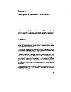
FIG. 1. Streamlines of the usual Fofonoff inertial flow (b), solution of (4.1) with zero circulation and an energy E/ L 2 5 0.189 m 2 s22 . It has been obtained as the final state of the relaxation equations (run MEPm2.0) from the initial condition shown in (a). The contour values are expressed in Sverdrups (Sv [ 10 6 m 3 s21 ), corresponding to c 5 2000 m 2 s21 , with our layer thickness 500 m.

lation: it is the well-known Fofonoff inertial flow, represented in Fig. 1b, which we shall now briefly recall. In the basin interior the PV is dominated by the term by, so (4.1) implies

b(y 2 y 0 ) 5 B 2c .

(4.2)

The corresponding velocity is therefore a constant westward current u 5 2b/B 2 . This flow must return along boundary jets in which the vorticity Dc is of the same order as by and is dominated by the derivative with respect to the coordinate z normal to the wall. This yields ] 2c 2 B 2c 5 0 ]z 2

(4.3)

with the straightforward solution

c 5

b(y 2 y0 ) [1 2 exp(2Bz )]. B2

(4.4)

The constants B and y 0 are determined by the energy E and circulation G 5 ∫ v d 2r. The circulation is also given by the contour integral of the velocity along the boundaries, and this velocity is ]c /]z(z50) 5 b(y 2 y 0 )/B, from (4.4), with the boundary layer approximation y ø const. The energy is also dominated by the boundary jets. An energy density b 2(y 2 y 0) 2 /(4B3) per unit of length is obtained from (4.4), by integration of (]c /]z) 2/2 with respect to z. The integration of these quantities along the boundaries of a rectangular basin of length L (along x) and width aL yields

E aL 2

5

G5

(bL 2 ) 2

G2

24(BL)

8BL 3 a(1 1 a)

a(a 1 3) 1 3

bL 2 2y0 B

L

(1 1 a),

(4.5)

(4.6)

which determines the constants B and y 0 from the energy E and circulation G of the initial condition. For G 5 0, we get a symmetric circulation (y 0 5 0), as in Fig. 1b. The corresponding energy, E /aL 2 5 0.189 m 2 s22 , typical for the ocean, corresponds to BL 5 45 k 1. The condition of strong b effect, with the distinction between an interior flow and boundary jets, is therefore well satisfied. When G ± 0, (4.6) yields a larger value of B for the same energy, so this approximation is still better fulfilled. Using the b parameter defined by (2.8), relation (4.5) then states more generally that the relative boundary layer thickness 1/(BL) scales like E 2/3 b , so the boundary jet approximation LB k 1 is, indeed, valid when E b K 1. The inertial flow of Fig. 1b has been computed by the relaxation equations MEPm2 from the initial condition of Fig. 1a in the absence of forcing and friction. A large diffusivity is then used, as we are only interested in the final steady state. The energy, circulation and total potential enstrophy are conserved in this relaxation process, within the numerical error (typically 1‰ over the whole run). These results confirm that the Fofonoff solution is not only a solution of (4.1) but truly is an entropy maximum. The same final flow is alternatively

JUNE 1998

KAZANTSEV ET AL.

1027

FIG. 2. Free inertial organization with high-resolution computation (REF.0) and the MEP relaxation equations. (a) Streamlines of the stabilized state obtained after complex rearrangement (time t 5 6.5 yr, averaged over 125 days to eliminate the oscillating component, made of Rossby waves). (b) Final state predicted as the statistical equilibrium, from the complete relaxation equations (with three PV levels, run MEP3.0). (c) Scatterplot PV vs streamfunction, corresponding to the field in (a). (d) Scatterplot PV vs streamfunction corresponding to the field in (b).

obtained with the simplified relaxation equations MEPm1. We have similarly computed the free evolution for the reference computation, using a small (ordinary) diffusivity, as allowed by the high-resolution 20 km. The energy is not strictly conserved, due to viscous effects, but varies by no more than 20%. After a complex evolution, during a few years, we observe (see Fig. 2a) an organization into inertial gyres, with a weak westward current in the interior, closing along strong boundary jets. There is a significant analogy with the Fofonoff

flow predicted by the statistical theory. Notice in particular that the final gyres have the opposite sign as the initial vortices. This reversal indicates a clear trend toward the statistical equilibrium (the initial condition with the opposite velocity leads practically to the same final state). There is, however, a discrepancy with the Fofonoff flow due to the presence of a central region with a quiet mean flow. This is most clearly revealed by the plot of q versus c, shown in Fig. 2b. The PV is nearly uniform inside the gyres, with a step at c ø 0 corresponding to

1028

JOURNAL OF PHYSICAL OCEANOGRAPHY

the variation of the planetary vorticity without a corresponding change of c, due to the absence of mean velocity. Notice furthermore that about half of the energy remains as Rossby waves, superposed upon the mean flow shown in Fig. 2a. These waves decay only very slowly, so a true equilibrium has not been reached. Cummins (1992) has performed similar comparisons between the statistical equilibrium and high-resolution numerical simulations for different boundary conditions. For the super-slip boundary conditions, he finds better agreement with the Fofonoff solution. His initial condition is more random, which probably favors PV mixing. In any case, such computations of the free evolution clearly indicate a trend toward inertial Fofonoff gyres, at least in strongly stirred regions, which provides a first supporting evidence for the validity of our MEP parameterization. Notice however that the linear relationship (4.1) has been obtained only in the frame of the two-moment approximation. The case of the complete formulation will be discussed in the next subsection, but the result will be practically unchanged, so this subsection can be skipped in a first reading. b. Statistical equilibrium in the complete formulation At statistical equilibrium, the condition of vanishing fluxes J, expressed by (3.14), yields = lnr 5 2b(q 2 s)=c . Taking the difference with any reference PV level s 0 , this relation yields = ln[r(s, r)/r(s 0 , r)] 5 b(s 2 s 0 )=c . Then by space integration ln[r(s, r)/r(s 0 , r)] 5 b(s 2 s 0 )c 2 a(s), where we have introduced an integration constant a(s). We therefore recover the general condition of statistical equilibrium introduced by Robert and Sommeria (1991):

r(s, r) 5

E

exp(2a(s) 1 bsc )

.

(4.7)

exp(2a(s) 1 bsc ) ds

The probability of any PV level s depends on the position r only through the streamfunction so that q is also a function F of c ,

q 5 F(c ) [

E E

exp(2a(s) 1 bsc )s ds .

(4.8)

exp(2a(s) 1 bsc ) ds

Then the advective term in (3.4) vanishes, characterizing an inviscid steady flow. This generalizes the linear relationship (4.1) obtained with the two-moment approximation. The function F depends on the unknown parameter b, the inverse of a ‘‘temperature,’’ and function a(s), the ‘‘chemical potential’’ of the PV level s. These parameters are indirectly given by the integral constraints,

VOLUME 28

obtained from the conservation of the energy E, and of the global distribution g(s) of the PV levels

E

r(s, r) d 2 r 5 g (s)

(4.9)

for all s. These conserved quantities are set by the initial condition in the freely evolving case. As in the twomoments formulation, this problem has an infinite set of solutions, but only one solution (or very few) corresponds really to a maximum entropy. The MEP relaxation equations (3.2)–(3.4) and (3.10)–(3.12) provide an efficient tool to find such a statistical equilibrium: they maximize the entropy while conserving all the conserved quantities, g(s) and E. The equilibrium state obtained from our two-vortex initial state of Fig. 1a is represented in Fig. 2c. We use our relaxation model with a resolution e 5 80 km (run MEP3.0 in Table 1). Three vorticity levels have been chosen for the PV-level discretization; namely, 2bL, 0, and 1bL. Control runs with 11 levels appear to give very close results for the explicit flow c , which is the quantity of interest (but the local probability distribution of PV levels is then better represented). As in the previous two-moment formulation, the eddy viscosity A E is high so that equilibrium is quickly reached, but the result is independent of this coefficient. We observe that the relationship between PV and streamfunction is nearly linear, so the behavior is nearly the same as with the two-moment formulation. We have observed this result for various initial conditions with strong b effect (i.e., E b K 1), typical of oceanic motion. Notice however that in the opposite limit b 5 0 (Euler equations), a rich variety of equilibrium states has been obtained, depending on circulation, energy, and domain shape (Juttner et al. 1995; Chavanis and Sommeria 1996). For many of these states, the approximation of a linearized relationship between vorticity and streamfunction does not apply. It is therefore useful to understand how good and how general the linearized approximation is with a strong b effect. First notice that the statistical equilibrium always has the structure of the Fofonoff flow, even when F is nonlinear. Indeed, the statistical theory predicts in all cases that this relationship between PV and streamfunction is monotonic (Robert and Sommeria 1991). It is increasing for a positive temperature, b . 0, or decreasing for a negative temperature, b , 0 [taking into account that c was defined with the opposite sign in Robert and Sommeria (1991)]. We find with the relaxation equations that b is always positive in the presence of strong b effect so that F is an increasing function. As in the linear case, we can distinguish the basin interior in which

by 5 F(c ) and the boundary jets where

(4.10)

JUNE 1998

] 2c 2 F(c ) 5 0. ]z 2

(4.11)

The relation (4.10) for the interior determines a westward flow, like in the linear case, but its velocity is not necessarily uniform. We could also imagine a case b , 0, with an eastward flow in the interior, but it cannot match with the boundary jet, as shown below: it must oscillate in the whole domain. Our relaxation equations indicate that such oscillating solutions must be excluded as they are not entropy maxima. Equation (4.11), determining the inertial boundary layer, can be understood by analogy with the equation of an oscillator in classic mechanics: z is analogous to the time and c to the position. We can define a ‘‘potential,’’ V(c ) 5 2∫ 0c F(c9) dc9, and show that the ‘‘energy’’ (]c /]z) 2 1 V(c ) is independent of z. The potential V(c ) is either convex or concave since its derivative 2F is monotonic. The case of a decreasing function F corresponds to a potential well: starting with some initial ‘‘velocity’’ ]c /]z, the point will oscillate forever. By contrast, an increasing function F corresponds to a potential ‘‘bump,’’ and the point can stop at the potential maximum with ]c /]z 5 0, then matching with the bulk solution. Notice that since V(c ) is either convex or concave, there can be at most one ‘‘equilibrium’’ point c for which ]c /]z 5 0. This excludes the possibility of a free jet at statistical equilibrium since such a jet would separate two regions of the bulk with different c ). Therefore an intense detached eastward jet, like the Gulf Stream, can be only obtained in a state out of equilibrium. In conclusion, the statistical equilibrium always contains a westward current in the interior, closing through inertial boundary jets, very much like in the linear case. Moreover, we have found numerically that the function F is nearly linear, and we try now to understand why. Chavanis and Sommeria (1996) have shown that such a linear relationship can be obtained in the limit of strong mixing for which the probabilities r are close to uniform. This is not the case here: on the contrary, the PV is dominated by the planetary vorticity by so that the probability of a given PV level s is nonzero only around its corresponding latitude y 5 s/b. A linear relationship, F, can be alternatively obtained when r(s) is a Gaussian, as assumed in the two-moment formulation; this is the relevant case here. Namely,

r5

1029

KAZANTSEV ET AL.

1 Ï2pq2

[

exp 2

]

(s 2 B 2c 2 by0 ) 2 . 2q2

(4.12)

We must check whether this Gaussian density satisfies the constraint (4.9). With our assumption of a strong b effect, the global PV distribution g(s) corresponds in first approximation to the planetary vorticity by: each PV interval [s, s 1 ds] occupies the latitude range [s/b, (s 1 ds)/b], with a constant area L ds/b. The resulting probability distribution g(s) is therefore uniform in the

interval [2baL/2, baL/2], corresponding to the latitudinal range of the basin [2aL/2, aL/2]. The integral of r in (4.9) can be limited to the interior flow (which occupies most of the area). In the interior, (4.2) applies, so (4.12) can be stated explicitly as

r5

E

1 Ï2pq2

Therefore

E

[

exp 2

]

(s 2 by) 2 . 2q2

(4.13)

1`

r(s, r) d 2 r ø L

r(s, y) dy 5 L/b

2`

for 2abL/2 , s , abL/2. (4.14) We have replaced the integral bounds 6aL by 6` since we have assumed q 2 K (abL) 2 , so r(s, y) is only weakly dispersed around the latitude s/b. The condition (4.9) with a uniform global PV distribution g(s) in the interval [2baL/2, baL/2] is therefore satisfied to first approximation by the distribution (4.12). Moreover, we know that this solution maximizes the entropy for a given energy, circulation, and PV enstrophy (see §3b), which makes it the best candidate once the constraint (4.9) is satisfied. It would be interesting to derive this approximation more rigorously, by determining the deviations to this Gaussian distribution and its effect on the function F. We can nevertheless conclude that this approximation is good when q2 K (abL/2) 2 . In terms of the initial condition, this condition corresponds to an enstrophy ∫ v 2 d 2r small with respect to (abL/2) 2 . c. Statistical equilibrium with forcing and friction The ocean circulation is in reality the result of a global balance between forcing and friction. Nevertheless, in the limit of weak friction (E k K 1), we may expect that turbulent mixing should dominate the dynamics and maintain a statistical equilibrium. This equilibrium is still determined by (4.1), or more generally (4.7), but the constraints on the conserved quantities must be replaced by conditions of global balance between forcing and friction. In the two-moment formulation, this balance is simply written by space integration of (2.1), see (2.4), G 5 TF 2E 5 T F

E E

curlt d 2 r 5 2T F L(t 1 2 t 2 )

(4.15)

t · u d 2 r,

(4.16)

where we have denoted t 1 and t 2 the wind stress at the northern and southern boundaries, respectively. Clearly (4.15) has nonzero solutions only when the wind stress is positively correlated with the Fofonoff solution. With the classic double-gyre forcing (2.5), the stress is mainly eastward in the interior and westward along the northern and southern boundaries, just op-

1030

JOURNAL OF PHYSICAL OCEANOGRAPHY

VOLUME 28

FIG. 3. Single-gyre wind forcing in the half-basin, with the nominal acceleration t m 5 (10/p) 3 1027 s21 : comparison between a reference high-resolution run (REF.1), resolution 20 km (a), and the MEP parameterization (MEPm2v.1), resolution 80 km (b). Streamlines of the permanent flow obtained after a 5-yr spinup time are represented, contour interval 100 Sv.

posite to what is required. We can make the discussion more precise by explicitely solving (4.15)–(4.16), as follows. The velocity is constant in the interior, u 5 2b/B 2 from (4.2), so that the total work in the interior is just proportional to ∫ t dy. The forcing is unchanged by adding a constant to the wind stress (the curl is not modified, and the additional force is just balanced by a pressure gradient). Therefore we can assume ∫ t dy 5 0 without loss of generality, so that the work of the wind stess t · u is only effective in the boundary jets. This stress can be assumed uniform over the width of the jet, so that the work per unit length is proportional to the integral of the velocity across the jet. This integral is the streamfunction outside the jet, that is, the boundary value of the interior flow solution (4.2). Therefore the total work is just the circulation of c t along the boundary of the interior solution. At the eastern and western sides, the wind stress is orthogonal to the boundary with zero work, so the total work is determined by the northern boundary, with streamfunction denoted c1 , and by the southern boundary, with streamfunction denoted c2. The total work is therefore ∫ t · u d 2r 5 L(c1 t 1 2 c2 t 2 ). Then, using (4.2), (4.5)–(4.6), (4.15)–(4.16), we find BL 5

bL 2 a(a 1 3) X 3T F

y0 a13 52 X(t 1 2 t 2 ), aL 3(a 1 1)

(4.17) (4.18)

where X is solution of the equation a13 (t 2 t 1 ) 2 X 2 1 2(t 1 1 t 2 )X 2 1 5 0, (4.19) a11 2 which always has a single positive solution. For the standard double-gyre forcing (2.5), t 1 5 t 2 , 0, we obtain the limit B → ` so that there is no flow

at statistical equilibrium, in agreement with the simple argument given above. Another interesting case is obtained by taking the same forcing (2.5), but restricted to a single gyre, keeping, for instance, only the lower ‘‘half-basin.’’ Then t 1 5 2t 2 5 t m so that (4.17)–(4.19) reduce to BL 5

aÏ(a 1 1)(a 1 3) 6E b

!

y0 1 a13 52 , aL 3 a11

(4.20)

(4.21)

where we have used the b number E b defined by (2.9). For our half-basin a 5 1/2, (4.21) yields y 0 /(aL) ø 20.51: the statistical equilibrium is a single anticyclonic gyre with a strong eastward jet along the northern boundary, as shown in Fig. 3. The ratio of the domain width aL to the jet width B21 is then aBL 5 0.095E 21 b , so our initial hypothesis of a boundary jet, aBL k 1, is satisfied when E b K 0.1.

(4.22)

The validity of the statistical equilibrium also requires a condition of inertial flow: the balance between forcing and friction is global, with forcing and friction times much longer than the circulation time along the gyre. This circulation time is controlled by the slowest part in the interior, with velocity |u| 5 b/B 2 . The corresponding transit time is L/|u| and the velocity change due to the wind stress acceleration t m is then t m L/|u|. Assuming that this velocity change is small with respect to u, we obtain the condition for an inertial gyre u 2 k t m L. Using the result (4.20) and the definition (2.6) of the Ekman number, this condition becomes, for the halfbasin, E b k 0.11E 1/3 k .

(4.23)

The same analysis for the friction effect yields the con-

JUNE 1998

KAZANTSEV ET AL.

dition E b k 0.19E 1/2 k , which is generally less severe than the condition on forcing. Notice again that for the symmetric double-gyre forcing (2.5), the statistical equilibrium has zero velocity so that the condition of an inertial gyre can never be satisfied globally. There is also a more subtle condition of validity for the statistical equilibrium concerning the enstrophy balance in the forced case. Indeed, the global balance between forcing and friction requires in general that some turbulent fluctuations persist, assuring PV transfer across the streamlines. This is a difficulty since at statistical equilibrium there is no PV flux J q . Therefore there is no source of local fluctuations, and q 2 can only decay by friction, according to (3.30). Therefore the system must be always slightly out of equilibrium to maintain the PV fluctuations. An alternative possibility is a balance between forcing and friction along each streamline. Verkley and Zimmerman (1995) have analyzed the corresponding inertial gyres (at least in a particular case without boundary jets) and have found a nearly linear relationship between PV and streamfunction. Such an analysis may provide an additional justification for the selection of a Fofonoff flow in the inertial limit. Finally, we have made the assumption of a quasiGaussian probability distribution, leading to the linear relationship between PV and streamfunction. Numerical computations support this hypothesis, but it may be useful in more general cases to write the condition of statistical equilibrium with forcing and friction. The condition of energy stationarity is always given by (2.4). The condition of stationarity for the global probability distribution g(s) is obtained from (3.36):

E

curlt

]r 2 d r5 ]s

E

1

2

] s 2 by r d 2 r. ]s TF

(4.24)

Taking the primitive of this relation with respect to s yields

E

1

r curlt 2

2

s 2 by 2 d r50 TF

1031

counterrotating cells. Normally, this Gulf Stream–like jet is strongly unstable with mixed barotropic/baroclinic instabilities. In the present model, only barotropic instability would be acting subject to the constraint that the resolution is fine enough. Before considering this double-gyre case, we first consider a half-basin, taking only a single gyre. We indeed expect to make a closer connection with statistical equilibrium in this case, as discussed in subsection 4c. For each case, we first run a reference simulation (REF) at high resolution (e 5 20 km in both directions) with a weak ordinary viscosity of Laplacian type, as described in section 3e. The oceanic flow is spun up from rest under the influence of the wind forcing to a permanent regime, reached after about 5 years. After that, the model is integrated for 30 more years (in the case of the double-gyre forcing) in order to provide for an adequate time sequence for computing the time average flow fields and the eddy statistics. We then degrade the spatial resolution by a factor of 4 (resolution 80 km) and compare the results of different parameterizations defined in section 3 with the same physical parameters. The runs ORD correspond to the usual Laplancian viscosity at this coarse resolution 80 km. The MEP3 corresponds to the complete MEP formulation with a discretization in 3 PV levels. MEPm2 and MEPm1 correspond to the two-moment formulations introduced in section 3b, with or without a transport equation for the local vorticity variance q 2 . We have used either a uniform diffusivity (runs MEPm2) or a diffusivity depending on q 2 by (3.19) (runs MEPm2v). Each of these parameterizations depends only on a single free parameter, A E or k, determining the eddy diffusivity. As a general rule, we have chosen the minimal value of this coefficient, which prevents the development of numerical noise. When specified, we also present results with higher diffusivities to test the influence of this parameter. In general, the corresponding changes are weak as long as the diffusivity remains within a factor of 2 from the minimal value.

(4.25)

(the constant of integration has been determined by the condition of vanishing r for large s). The constraints (2.4) and (4.25) replace the conditions (3.7) and (4.9) of the free evolution case. 5. Application to a wind-driven oceanic basin We now study how the MEP parameterization performs in an actual oceanic model with forcing and friction. Different simulations have been performed, the details of which are presented in Table 1. The parameters not specified in the table are those introduced in section 2, which are common to all cases. We mostly consider the familiar double-gyre wind-forced box, which mimics an open ocean intense jet arising at midlatitudes at the convergence of the subpolar and the subtropical

a. The single-gyre wind forcing With our nominal forcing t m 5 10/p 3 1027 m s22 limited to the lower half-basin (2L/2 , y , 0), we observe the flow organization into a single gyre (Fig. 3a). After the spin up of about 5 years, a nearly steady state is reached: the relative vorticity and velocity fluctuations are typically 1024 . The jet is stabilized by the northern boundary and behaves quite differently from the classic two-gyre case discussed in the next subsection. This organization is in agreement with the statistical equilibrium dicussed in section 4c. An intense jet along the northern boundary has been predicted, with a width given by (4.20). The aspect ratio is a 5 1/2 and the b parameter E b 5 2 3 1022 , leading to a predicted jet width B21 5 L/10. The assumed condition (4.22) for

1032

JOURNAL OF PHYSICAL OCEANOGRAPHY

VOLUME 28

FIG. 4. As in Fig. 3 but with a wind forcing five times smaller, t m 5 (2/p) 3 1027 s21 , for which an inertial gyre coexists with a southern region controlled by the Sverdrup balance (runs REF.2 and MEPm2v.2); contour interval 3 Sv.

a thin jet is not very well satisfied but is still good for a first approximation. We notice also that, with our Ekman number E k 5 0.63 3 1023 , the condition (4.23) for a global inertial flow is only marginally satisfied (by a factor of 2). The predicted maximum velocity along the northern boundary is, from (4.4), bL/(2B) 5 16 m s21 , and the velocity in the interior 2b/B 2 5 3.2 m s21 , while the corresponding numerical values are 11.6 m s21 and 2.7 m s21 , respectively. Therefore the statistical equilibrium prediction is only a first ap-

proximation, and we clearly observe some discrepancy in the southern part of the basin. Accordingly, the total energy is E /(aL 2 ) 5 4.1 m 2 s22 , about half the value E /(aL 2 ) 5 10 m 2 s22 predicted by (4.16). As expected, this flow is well reproduced by the MEPm2v computation (Fig. 3b). However, good agreement is also obtained with the other parameterizations. Due to the weakness of the fluctuations and the relatively large jet width, the numerical modeling appears to be only weakly sensitive to the subgrid-scale parameterization.

FIG. 5. Effects of poor turbulence parameterizations at coarse resolution for the same condition as in Fig. 4, streamlines are represented with contour interval 3 Sv (a). Two-moment formulation with uniform diffusivity, run MEPm2.2; (b) Complete formulation with uniform diffusivity, run MEP3.2; (c) MEP parameterization with uniform q 2 , run MEPm1.2; and (d) ordinary diffusivity, run ORD.2.

JUNE 1998

KAZANTSEV ET AL.

1033

FIG. 6. The double-gyre wind forcing: reference computation with resolution 20 km (REF.3) (left) compared with the two-moment MEP parameterization with resolution 80 km (MEPm2v.3.b) (right). (a) and (b) Examples of instant streamlines, contour interval 15 Sv, from 2135 to 165 Sv (REF), and from 2165 to 150 Sv (MEP); (c) and (d) streamlines of the 30-yr averaged velocity field; contour interval 10 Sv, from 280 to 190 Sv (REF), and from 2100 to 90 Sv (MEP).

In order to obtain velocities more typical of oceanic data we have reduced the forcing by a factor of 5, choosing t m 5 (2/p) 3 1027 m s22 . Then the condition (4.23) of a global inertial flow is no longer satisfied. We observe again the spin up ending in a nearly steady flow, but the inertial gyre is limited to a northern region (Fig. 4). In the southern part, the Sverdrup balance (2.10) occurs instead, with negligible inertial effects. Notice

that the mean energy is E /(aL 2 ) 5 40 3 1024 m 2 s22 , 1000 times weaker than with our nominal forcing. In the statistical equilibrium results of section 4c, energy is dominated by the boundary jets with velocity ;t m and width ;t m so that energy would scale like t m3 and should be 125 times smaller than with the nominal forcing. An additional reduction is due to the smaller size of the inertial gyre.

1034

JOURNAL OF PHYSICAL OCEANOGRAPHY

VOLUME 28

FIG. 7. The double-gyre wind forcing: reference computation with resolution 20 km (REF.3) (left) compared with the two-moment MEP parameterization with resolution 80 km (MEPm2v.3.b) (right). (a) Streamfunction rms, contour interval 10 Sv; (b) eddy kinetic energy, ^u9 2 1 y 9 2 & 5 (^u 2 & 2 ^u& 2 ) 1 (^y 2 & 2 ^y & 2 , contour interval 0.2 m 2 s22 , from 0 to 2.4 m 2 s22 (REF), and from 0 to 2 (MEP); (c) explicit vorticity fluctuations (rms), with contour interval 0.3 3 1025 s21 from 0.3 3 1025 s21 to 3 3 1025 s21 (REF), and from 0.3 3 1025 s21 to 2.7 3 1025 s21 (MEP); (d) implicit vorticity fluctuations, variance q 2 (defined only for the MEP), with contour interval 10 210 s22 , from 10210 s22 to 5 3 10210 s22 .

The MEPm2v, with variable diffusivity, reproduces well the reference computation, as shown in Fig. 4b. With a constant diffusivity, the inertial gyre is unchanged but the southern region is somewhat distorted by diffusive effects, as seen in Fig. 5a (to compare with the reference case Fig. 4a). This test confirms that it is useful to in-

troduce a variable diffusivity when the flow activity is highly inhomogeneous. We have also checked that, like in the free inertial case, the complete formulation (MEP3) gives a result very close to the two-moment formulation, as seen by comparing Figs. 5a and 5b. The parameterization MEPm1 performs poorly, as

JUNE 1998

KAZANTSEV ET AL.

1035

Fig. 7. (Continued )

shown in Fig. 5c. The coefficient bq 2 of the friction term bq 2=c in (3.21) is then uniform, which severely perturbs the southern region. By contrast in MEPm2, q 2 satisfies the transport equation (3.22) and remains in the inertial gyre. Therefore the friction term remains only ‘‘where it is needed,’’ correcting the diffusion without impacting the more quiet region. The effect of an ordinary viscosity is still worse, as shown in Fig. 4d, with a strongly overestimated energy. Notice that our superslip boundary condition can be a source of energy, but in any case an ordinary viscosity is clearly inap-

propriate to describe the inertial boundary jets with a coarse resolution. b. The double-gyre wind forcing We now consider the more realistic double-gyre case in the square basin (with the nominal forcing t m 5 10/p 3 1027 m s22 ). The flow remains strongly unsteady in the permanent regime, which greatly contrasts with the half-basin case. Furthermore, the typical velocity is

1036

JOURNAL OF PHYSICAL OCEANOGRAPHY

much lower than in the half-basin, with a mean energy about 30 times smaller, E /L 2 5 0.108 6 0.05 m 2 s22 (the uncertainty corresponds to the typical fluctuations). Therefore to a first approximation, the flow can be considered as zero, in agreement with the prediction for the global statistical equilibrium (see §4c). However, we are of course interested in this residual flow and use the statistical mechanics in the form of eddy parameterization. We compare in Fig. 6 results obtained with the reference computation (REF.3), left, and the MEP (run MEPm2v.3.a), right. We first show an example of instantaneous streamfunction field (Fig. 6a). The mean streamfunction, shown in Fig. 6b, is in good agreement with the MEPm2 computation. We observe the western boundary jets, detaching into a free jet (the ‘‘Gulf Stream’’), surrounded by inertial gyres. The remaining of the mean flow is controlled by the Sverdrup balance, while variability is due to Rossby waves emitted by the instabilities of the detached jet. All these features are well reproduced with the coarse resolution by the MEPm2v parameterization. The mean energy is E /L 2 5 0.127 6 0.05 m 2 s22 (about 15% higher than for the reference computation). Although the flow is globally out of statistical equilibrium, we can estimate the main flow features by a simple model, assuming some statistical equilibrium restricted to the inertial gyres on each side of the detached jet. We enclose by thought each gyre in a box with the length L9 of the detached jet (to determine eventually). We take an aspect ratio a 5 1/2 for which the wind forcing maintains a single gyre at statistical equilibrium (as seen in section 4c). The gyre is characterized by a parameter B, which determines the velocity 2b/B 2 in its interior. This parameter also determines the velocity in the (southern half ) detached jet, by (4.4) with y 2 y 0 5 L9/2. Unlike in the isolated basin, the energy of the gyre does not result from a balance betwen forcing and friction, since the free jet carries energy away, and emits it as Rossby waves (eventually dissipated by bottom friction in the whole basin). This transport is an energy sink for the gyre, and dominates the bottom friction. The energy flux carried by the (half ) jet is ∫ U 3/2 dy 5 b 3 L9 3 /(48B 4 ), which must be balanced by the work of the wind stress, L9t m ∫ U dy 5 bL9/(2B 2 ). Equating these two quantities gives B 2 5 b 2 L9/(24t m ).

(5.1)

The length L9 can be determined by stating that the gyre occupies the largest domain in which the condition of inertial flow can be sustained. This corresponds to the equality of the transit time and the forcing time, u 2 5 t m L9, with the velocity of the interior flow u 5 2b/B 2 . This yields the second condition

b 2 /B 4 5 t m L9.

(5.2)

Combining (5.1) and (5.2), we find the following laws for the jet length L9, its half-width B21 , the maximum velocity in the jet Umax , and half flow rate c1 of the jet:

VOLUME 28

22/3 L9 ø 4 3 3 2/3t 1/3 5 800 km, m b

B21 ø L9/5 5 160 km, Umax ø 7.06t b 2/3 m

21/3

(5.4)

5 1.2 m s ,

c1 ø 12t m /b 5 100 Sv

(5.3)

21

(Sv [ 10 6 m 3 s21 ).

(5.5) (5.6)

Notice that the results are independent of the basin width and friction time. However, the total energy E of the flow, including the field of Rossby waves, must depend on bottom friction. Indeed, the rate of energy dissipation 2E /T F equals the production by the wind stress, twice the production bL9/(2B 2 ) for the half-jet, so that E /L 2 . 11.5T F b21 L22 t m 5 0.23 m 2 s22 . (5.7) The numerical predictions with our parameters have been quantified. The total energy is overestimated by a factor of 2, but the predicted length and velocity of the jet are in good agreement with the numerical computations (see Fig. 10). The total jet flow rate predicted by (5.6) is 200 Sv, also very close to the result of the computation 180 Sv (corresponding to the difference between the maximum and minimum streamfunction in Fig. 6b, 690 Sv). This supports the idea that the effect of turbulence is to drive the system toward a statistical equilibrium, which is approached in the inertial gyres. A critical evaluation of the MEP is provided by the comparison of the variability fields with the reference computation. The rms of the streamfunction ^(c 2 ^c&) 2 &1/2 (where ^ · & denotes a 30-yr time average) is compared in Fig. 7a. This field characterizes the jet fluctuations in the central western part, and the intensity of the radiated Rossby waves. The MEP overestimates these fluctuations by about 20%, but reproduces well the overall pattern. The eddy kinetic energy field, defined as ^u9 2 1 y 9 2 & 5 (^u 2 & 2 ^u& 2 ) 1 (^y 2 & 2 ^y & 2 ), is represented in Fig. 7b, also showing good agreement. Finally, the field of vorticity fluctuation ^v 2 &1/2 is shown in Fig. 7c (left) and is compared with the explicit vorticity fluctuations ^v 2 &1/2 in the MEP (right). The MEP also provides a field of implicit fluctuations q 2 with a similar distribution around the jet region (Fig. 7d). The explicit fluctuations are a little lower in the MEP than in the reference computation, but the total v 2 1 q 2 overestimates the fluctuations. Notice, however, that a reference computation with higher resolution would probably contain higher vorticity fluctuations, although with little influence on the velocity fields (which smoothes out the finescale vorticity fluctuations). Figure 8 extends the comparison to the PV eddy fluxes (^y 9q9&) in the meridional direction. The dynamical significance of these eddy fluxes has been long recognized (Rhines and Holland 1979; Holland and Rhines 1980) since their divergence rectifies the mean flow. In the case of the reference simulation (left side), we consider that the flux is explicitly obtained as ^y 9q9&. In the case of the MEP simulation (right side), we add the explicit part ^y 9q9& and the y component to the implicit

JUNE 1998

KAZANTSEV ET AL.

1037

FIG. 8. Meridional eddy flux of potential vorticity ^y 9q9& (30-yr averaged), with the double-gyre wind forcing. Reference computation with resolution 20 km (REF.3) (left) compared with the two-moment MEP parameterization with resolution 80 km (MEPm2v.3.b) (right). The isovalue contours are represented in (a) from 5 3 1026 to 245 3 1026 m s22 , with interval 5 3 1026 m s22 in the first slice, within 300 km of the western side, and with interval 0.3 3 1026 m s22 in the second slice, in the range (300–1500 km). The fluxes are much weaker in the eastern part of the basin. The same representation is used in (b), with contours from 5 3 1026 to 230 3 1026 m s22 in the first slice. The PV flux averaged in longitude x^y 9q9& is represented in (c) for the reference computation. For the corresponding MEP computation, in (d), we represent by the solid curve the total flux x^y 9q9& 1 x^J q & , the sum of the parameterized subgrid-scale eddy flux x^J q & (dashed curve), and the effect of explicit variability.

1038

JOURNAL OF PHYSICAL OCEANOGRAPHY

VOLUME 28

FIG. 9. Spurious mean flow obtained with a poor turbulence parameterization at coarse resolution for the double-gyre wind forcing (cf. the reference computation in Fig. 6b). (a) Ordinary viscosity (run ORD.3.1500); (b) MEP diffusivity with excessive diffusivity (run MEPm2v.3.d); contour interval 10 Sv from 2130 to 130 Sv in (a) and from 2170 to 170 Sv in (b).

flux J q , given by (3.6). The maps of the PV flux for the reference (Fig. 8a) and MEP computation (Fig. 8b) compare very well. The strongest PV flux is located at the middle of the western boundary and corresponds to a latitudinal oscillation of the jet detachment point. We can estimate the corresponding PV transport, using our model results (5.4)–(5.5). Indeed at the middle of the western boundary, the time-averaged velocity is zero, but the jet is either northward (positive) with velocity Umax and vorticity 2bL/2 (coming from the lower corner of the basin) or southward with vorticity 1bL/2 (coming from the upper corner). In both cases, it corresponds to a PV flux

is indeed 2t m 5 20.64 3 1026 m s22 , in reasonable agreement with the peak of Fig. 8c. There is some discrepancy with the coarse resolution (Fig. 8d), but with the same general trends. The implicit flux is also plotted in Fig. 8d, but is much weaker than the explicit flux: the MEP parameterization does not directly model the PV flux due to the oscillations of the detached jet. However it has an essentiel indirect influence by providing a correct simulation of the explicit eddies, preserving their energy and PV.

(y 9q9)extr ø UmaxbL/2 5 7.06t m2/3b 2/3 L/2

In the two-gyre case, we have found similar results with a variable diffusivity (MEPm2v) or with a uniform diffusivity (MEPm2). We also have good agreement between the two-moment formulation and the complete formulation (MEP3). We now discuss typical defects of other parameterizations, which help to put the performance of MEPm2 in perspective. An ordinary viscosity with the same resolution of 80 km yields the mean flow of Fig. 9a, which is not good (cf. the reference case of Fig. 6b). The jet flux is excessive (260 Sv), and the velocity is too high (Fig. 10e). Moreover the fluctuations are completely damped by viscosity, even for the minimum value (1000 m 2 s21 ) necessary to avoid numerical noise at this resolution. MEPm1 performs better than ordinary viscosity. The detached jet is unstable (see the snapshot of Fig. 11a),

5 25 3 1025 m s22 .

(5.8)

This provides a good estimate of the extremum PV flux in Fig. 8a. Weaker extrema are also seen east of the detachment point and are linked with jet meanders. The resulting longitude averaged fluxes are plotted in Figs. 8b and 8c. There is globally a strong PV flux from the northern half-basin toward the southern half-basin, as indicated by the strong central peak (this flux is mainly located near the western boundary). The wind produces a circulation in each half-basin with the same rate 2Lt m but opposite sign. A small proportion (about 2%) of this circulation is lost by bottom friction, but most of the production is balanced by the PV flux between the two half-basins. The corresponding x-averaged flux

c. Influence of the parameterization type and eddy diffusivity

JUNE 1998

KAZANTSEV ET AL.

1039

FIG. 10. Mean velocity along the jet center (y 5 0) vs longitude, with the double-gyre forcing, for different parameterizations. In each graph the results obtained with the coarse resolution 80 km, with different diffusivities, are compared with the reference computation at resolution 20 km (run REF.3, solid line). (a) MEP with two moments and variable diffusivity (MEPm2v); (b) MEPm2 with two moments, constant diffusivity; (c) MEP3 with three PV levels; (d) MEPm1 with uniform q 2 ; (e) ordinary viscosity (ORD).

1040

JOURNAL OF PHYSICAL OCEANOGRAPHY

VOLUME 28

FIG. 11. Spurious behavior for the parameterization with uniform q 2 , double-gyre forcing, run MEPm1.3.1500 (cf. the reference computation in Figs. 6 and 7). (a) Snapshot of the streamlines, contour interval 15 Sv, from 2180 to 195 Sv; (b) streamlines of the 10-yr averaged flow, contour interval 10 Sv, from 2100 to 100 Sv; (c) streamfunction rms, contour interval 10 Sv from 0 to 130 Sv; (d) eddy kinetic energy ^u9 2 1 y 9 2 & 5 (^u 2 & 2 ^u& 2 ) 1 (^y 2 & 2 ^y & 2 , contour interval 0.1 m 2 s 2 2, from 0 to 1.1 m 2 s22 .

and the mean flow is reasonably well computed (streamlines in Fig. 11b and velocity profiles in Fig. 10d). However, the fluctuation fields for the streamfunction (Fig. 11c) and velocity (Fig. 11d) are not well represented (cf. the reference computations of Figs. 7a and 7b, respectively). All the results somewhat depend on the chosen diffusivity, and we now discuss the influence of this pa-

rameter. We have found that a good evaluation of a parameterization is obtained by plotting the velocity along the jet center (y 5 0) and comparing it with the reference computation (solid curve in Fig. 10). For each kind of parameterization, we first choose the minimum diffusivity that prevents growth of numerical noise and compare with results at higher diffusivity. With the parameterization MEPm2v, this minimum diffusivity is

JUNE 1998

KAZANTSEV ET AL.

obtained with k 5 0.62 3 1022 but a slightly better result is obtained for k 5 0.94 3 1022 , the value we have chosen in Figs. 6–8. The result with k 5 1.25 3 1022 is still close, but the system switches to a different regime for k 5 3.12 3 1022 , with the field of Fig. 9b. As already stated, the results with a uniform diffusivity (MEPm2), Fig. 10b, and with the complete formulation (MEP3), Fig. 10c, are in close agreement with the reference computation (provided that the diffusivity is not too far from the minimum value). The corresponding results with MEPm1 are less good, Fig. 10d, and the results with ordinary viscosity still worse (Fig. 10e). 6. Conclusions We have applied an equilibrium statistical theory for continuous PV fields to a barotropic model of an ocean basin. The result of a free inertial evolution appears very close to the classic Fofonoff solution, obtained earlier with truncated spectral models or selective decay hypothesis. Our procedure is, however, more general as it takes into account all the conservation laws of the system. In particular, it applies also to self-organization into coherent vortices in the absence of the b effect, unlike the truncated spectral model. The Fofonoff flow is necessarily eastward in the basin interior, with strong westward boundary jets. This statistical equilibrium can be maintained by wind forcing when it is compatible with this flow direction, like in the considered half-basin case (sections 4c and 5a). However, the usual double-gyre wind forcing has the wrong direction, and it cannot maintain a global statistical equilibrium. Such an equilibrium is approached only in the recirculating gyres on each side of the central jet, as already noticed by many authors (e.g., Ierley and Young 1988). We have formalized this idea in a simple model (§5b), which correctly estimates the main flow features. As the system is generally not in a global statistical equilibrium, we consider that the effect of turbulence is to drive the system toward equilibrium: it provides the maximum entropy production (MEP) with appropriate constraints. This is a practical implementation of the ideas advocated by Holloway (1992) for eddy parameterization. Our parameterization can be considered as mixing PV, in a similar spirit as Marshall (1984) but with the constraint of energy conservation. The complete MEP formulation involves a new variable, the PV level s, but a coarse three-level discretization (MEP3), involving only two independent values, appears to be sufficient. A more convenient possibility is to work with the successive moments of the PV distribution, using a local maximum entropy closure. The truncation limited to the two first moments is equivalent to assuming a local Gaussian PV probability distribution and it provides coupled transport equations for the PV q and local enstrophy q 2 (MEPm2). In typical oceanic conditions, with local vorticity fluctuations much small-

1041

er than the planetary vorticity bL, we find that this twomoment formulation yields results close to the complete formulation, both for the statistical equilibrium and for the wind-driven case. The MEP procedure does not determine the eddy diffusivity, but simple considerations lead us to a proportionality in the local vorticity rms (q 2 )1/2 . The results obtained with this MEPm2v parameterization compare well with a computation at higher resolution in terms of mean currents, fluctuations, and eddy transport. By comparison, an ordinary viscosity with the same resolution gives only a crude mean flow, without any variability. The simplified MEPm1 formulation, assuming that q 2 is uniform, is also defective, although less severely. Of course the success of the MEPm2v parameterization is obtained at the price of a more complex set of equations. The computing time with the MEPm2v modeling appears to be about six times longer than for the vorticity equation with ordinary viscosity at the same resolution (but it could be probably optimized). However, a factor of 4 in resolution typically infers a factor 4 3 in computational cost. As a practical result, the simulation MEPm2v is about ten times shorter than the corresponding simulation REF. Beyond the gain in computation time and storage, this parameterization offers perspectives for improving the physical modeling. For instance, the boundary condition (3.24) is naturally brought by the theory without arbitrary assumption: it arises from the absence of production or dissipation of PV at the boundaries. Furthermore, any force applied to the system can be decomposed into an explicit and subgrid component, modifying the distribution of PV levels. The influence of small-scale topography or wind variability could then be introduced quite naturally. The most direct application of our results is probably the link with the ‘‘Neptune’’ effect of Holloway (1992), obtained when the b effect is due to the bottom topography instead of planetary vorticity (§3c). The introduction of this effect in actual oceanographic modeling has been proven useful, but it relied on several arbitrary parameters. We specify these parameters, relating them to the eddy diffusivity, and provide a systematic derivation of this parameterization. The barotropic vorticity equation is clearly of limited scope for modeling the real ocean. The generalization of the MEP eddy viscosity to a stratified fluid must be undertaken to really prove its usefulness. There is no formal obstacle for this generalization within the quasigeostrophic approximation, provided the resolution is finer than the radius of deformation. The MEP basic principle applies to the isopycnal mixing without further assumption on diapycnal exchanges. For a cutoff scale larger than the radius of deformation, the subgrid eddies will contain a significant part of the energy, unlike in the barotropic case, so that an additional equation for the eddy energy would be necessary, in replacement of the constraint (3.8).

1042

JOURNAL OF PHYSICAL OCEANOGRAPHY

Acknowledgments. We have benefitted from a continuous collaboration with R. Robert and coworkers at Laboratoire d’Analyse Nume´rique de Lyon. Parts of this work have been made possible owing to support by the Direction des Recherches et Etudes Techniques under Contract 91/140 and by the Programme Atmosphe`re et Oce´an a` Me´soe´chelle of CNRS and IFREMER. All the contour plots in this paper have been prepared using the Grid Analysis and Display System developed at the Department of Meteorology of the University of Maryland. REFERENCES Alvarez, A., J. Tintore´, G. Holloway, M. Elby, and J. M. Beckers, 1994: Effect of topographic stress on circulation in the western Mediterranean. J. Geophys. Res., 99(C8), 16 053–16 064. Arakawa, A., 1966: Computational design for long term numerical integration of the equations of fluid motions: Two-dimensional incompressible flow. Part 1. J. Comput. Phys., 1, 119–143. Basdevant, C., and R. Sadourny, 1983: Mode´lisation des e´chelles virtuelles dans la simulation nume´rique des e´coulements turbulents bidimensionnels. J. Me´ca. Th. Appl. (Special issue), ‘‘Two-dimensional turbulence,’’ 243–269. Bretherton, F. P., and D. B. Haidvogel, 1976: Two-dimensional turbulence above topography. J. Fluid Mech., 78, 129–154. Carnevale, G. F., and J. S. Frederiksen, 1987: Nonlinear stability and statistical mechanics of flow over topography. J. Fluid Mech., 175, 157–181. Chavanis, P., and J. Sommeria, 1996: Classification of self-organized structures in two-dimensional turbulence: The case of a bounded domain. J. Fluid Mech., 314, 267–297. , and , 1997: A thermodynamical approach to small scale parameterization in 2D Turbulence. Phys. Rev. Lett., 28, 3302– 3305. Cummins, P., 1992: Inertial gyres in decaying and forced geostrophic turbulence. J. Mar. Res., 50, 545–566. , and G. Holloway, 1994: On eddy–topographic stress representation. J. Phys. Oceanogr., 24, 700–706. Fofonoff, N. P., 1954: Steady flow in a frictionless homogeneous ocean. J. Mar. Res., 13, 254–262. Gent, P. R., and J. C. McWilliams, 1990: Isopycnal mixing in ocean circulation models. J. Phys. Oceanogr., 20, 150–155. Griffa, A., and R. Salmon, 1989: Wind driven ocean circulation and equilibrium statistical mechanics. J. Mar. Res., 47, 457–492. Holland, W. R., 1978: The role of mesoscale eddies in the general circulation of the ocean—numerical simulations using a winddriven quasigeostrophic model. J. Phys. Oceanogr., 8, 363–392. , and P. B. Rhines, 1980: An example of eddy induced ocean circulation. J. Phys. Oceanogr., 10, 1010–1031. Holloway, G., 1986: Eddies, waves, circulation and mixing: Statistical geofluid mechanics. Annu. Rev. Fluid Mech., 18, 91–147. , 1992: Representing topographic stress for large-scale ocean models. J. Phys. Oceanogr., 22, 1033–1046. Ierley, G., and W. Young, 1988: Inertial recirculation in a b-plane corner. J. Phys. Oceanogr., 18, 683–689.

VOLUME 28

Jespersen, D. C., 1974: Arakawa’s method is a finite-element method. J. Comput. Phys., 16, 383–390. Juttner, B., A. Thess, and J. Sommeria, 1995: On the symmetry of self-organized structures in two-dimensional turbulence. Phys. Fluids, 7, 2108–2110. Kraichnan, R. H., and D. Montgomery, 1980: Two-dimensional turbulence. Rep. Prog. Phys., 43, 547–617. Kuz’min, G. A., 1982: Statistical mechanics of the organisation into two-dimensional coherent structures. Structural Turbulence, M. A. Goldshtik, Ed., Acad. Nauk CCCP Novosibirsk, Institute of Thermophysics, 103–114. Le Provost, C., and J. Verron, 1987: Wind-driven ocean circulation transition to barotropic instability. Dyn. Atmos. Oceans, 11, 175– 201. Marshall, J. C., 1984: Eddy–mean flow interaction in a barotropic ocean model. Quart. J. Roy. Meteor. Soc., 110, 573–590. Michel, J., and R. Robert, 1994: Statistical mechanical theory of the Great Red Spot of Jupiter. J. Stat. Phys., 77, 645–666. Miller, J., 1990: Statistical mechanics of Euler equations in two dimensions. Phys. Rev. Lett., 65, 2137–2140. Montgomery, D., and G. Joyce, 1974: Statistical mechanics of negative temperature states. Phys. Fluids, 17, 1139–1145. Muller, P., and G. Holloway, 1989: Parameterization of small-scale processes. Proc. Aha Hulikoa Hawaiian Winter Workshop, Honolulu, HI, 341–354. Onsager, L., 1949: Statistical hydrodynamics. Nuovo Cimento Suppl., 6, 279–287. Rhines, P. B., and W. R. Holland, 1979: A theoretical discussion of eddy-driven mean flows. Dyn. Atmos. Oceans, 3, 289–325. Robert, R., 1990: Etat d’e´quilibre statistique pour l’e´coulement bidimensionnel d’un fluide parfait. C. R. Acad. Sci. Paris, 311, Se´rie I, 575–578. , and J. Sommeria, 1991: Statistical equilibrium states for twodimensional flows. J. Fluid Mech., 229, 291–310. , and, , 1992: Relaxation towards a statistical equilibrium state in two-dimensional perfect fluid dynamics. Phys. Rev. Lett., 69 (19), 2776–2779. , and C. Rosier, 1997: The modelling of small scales in 2D turbulent flows: A statistical mechanics approach. J. Stat. Phys., 86, 481–515. Salmon, R., G. Holloway, and M. C. Hendershott, 1976: The equilibrium statistical mechanics of simple quasi-geostrophic models. J. Fluid Mech., 75, 691–703. Sommeria, J., C. Nore, T. Dumont, and R. Robert, 1991: The´ orie statistique de la Tache Rouge de Jupiter. C. R. Acad. Sci. Paris, 312, 999–1005. Strang, G., and G. J. Fix, 1973: An Analysis of the Finite Element Method. Prentice-Hall, 306 pp. Verkley, W. T. M., and J. T. F. Zimmerman, 1995: A series solution of the nonlinear wind-driven ocean circulation and its inertial limit. J. Fluid Mech., 295, 61–89. Wang, J., and G. K. Vallis, 1994: Emergence of Fofonoff states in inviscid and viscous ocean models. J. Mar. Res., 52, 83–127. Welander, P., 1973: Lateral friction in the ocean as an effect of potential vorticity mixing. Geophys. Fluid Dyn., 5, 101–120. Zou, J., and G. Holloway, 1994: Entropy maximization tendency in topographic turbulence. J. Fluid Mech., 263, 361–374.