Aug 7, 2015 - The output scores of a neural network classifier are converted to probabilities via normalizing over the scores ...... Curran Associates, Inc., 2014.
Sublinear Partition Estimation
arXiv:1508.01596v1 [stat.ML] 7 Aug 2015
Pushpendre Rastogi Benjamin Van Durme Johns Hopkins University
Abstract The output scores of a neural network classifier are converted to probabilities via normalizing over the scores of all competing categories. Computing this partition function, Z, is then linear in the number of categories, which is problematic as real-world problem sets continue to grow in categorical types, such as in visual object recognition or discriminative language modeling. We propose three approaches for sublinear estimation of the partition function, based on approximate nearest neighbor search and kernel feature maps and compare the performance of the proposed approaches empirically.
1
Introduction
Neural Networks (and log-linear models) have out-performed other machine learning frameworks on a number of difficult multi-class classification tasks such as object recognition in images, large vocabulary speech recognition and many others [19, 10, 25]. These classification tasks become “large scale” as the number of potential classes/categories increases. For instance, discriminative language models need to choose the most probable word from the entire vocabulary which can have more than 100,000 words in case of the English language. And in the field of computer vision, the latest datasets for object recognition contain more than 10,000 object classes and the number of categories is increasing every year [5]. In certain applications neural networks may be used as sub-systems of a larger model in which case it may be necessary to convert the unnormalized score assigned to a class by a neural network to a probability value. To perform this conversion we need to compute the so-called Partition Function of a neural network which is just a sum of the scores assigned by the neural network to all the classes. Let N be the number of output classes and let q, vi ∈ Rd where vi represents weights of ith class. Also, let ui be the score of the ith class, i.e. ui = vi · q then the partition function Z(q) is defined as: Z(q) =
N X
exp(ui )
(1)
i=1
The problem of assigning a probability to the most probable class can be stated as: Find, ˆı = arg max ui i
p(ˆı) =
exp(uˆı ) Z(q)
(2) (3)
Recently, [21, 17, 3] have presented methods for solving (2) by building upon frameworks for performing fast randomized nearest neighbor searches such as Locality Sensitive Hashing and Randomized k-d trees. This paper presents methods for estimating the value of Z(q) required in (3). While brute force parallelization is one effective strategy for reducing the time needed for this computation our goal is to estimate the partition function in asymptotically lesser runtime. 1
2
Previous Work
A number of techniques have been used previously for speeding up the computation of the partition function in artificial neural networks. Computational efficiency of the normalizing step seems to be especially important for these tasks because of the large size of vocabulary needed to achieve state of the art performance in these tasks. The prior work can be categorized by the technique it uses as follows: Importance Sampling: The partition function can be written as Z = N E[exp(ui )] where the distribution of i is uniform over [1, . . . , N ]. However, the attempts to estimate Z by simply drawing k samples from the uniform distribution and replacing the expectation by its sample estimate are marred by the high variance of the estimate. [4] were the first to use importance sampling for reducing the variance of the sample average estimator. Their aim was to speed up the training of neural language models and they used an n-gram language model as the proposal distribution. Though they do not use their method for actually computing the partition function at inference time, their method could be easily extended for that purpose. The problem however with their method is that it requires the use of an external model for constructing the proposal distribution. Such an external model requires extra engineering and knowledge, specific to the problem domain, that may not be available. Hierarchical decomposition: [13] introduced a method for breaking the original N -way decision problem into a hierarchical one such that it requires only O(log(N )) computations. That method requires a change in the model from a single decision problem into a chain of decision problems computed over a tree. Also, since there is no a priori single most preferable way of growing a tree for doing this computation therefore an external model is needed for creating the hierarchical tree. Self-Normalization: Some of the prior work side-steps the problem of computing the partition function and trains neural networks with the added constraint that the partition function should remain close to 1 for inputs seen during test time. [14] used Noise Contrastive Estimation1 with a heuristic to clamp the values of Z to 1 during training. They demonstrated empirically that by doing so the partition function at test time also remained close to 1 though they did not provide any theoretical analysis on how close to 1 the value of the partition function remains at test time. 2
On the other hand, [6] added a penalty term log (Z(q)) to the training objective of the neural network and empirically demonstrated on a large scale machine translation task that they do not suffer from a large loss in accuracy even if they assume that the value of the partition function is close to 1 for all inputs at test time. Recently, [1] showed that after training on n training examples, with probability�1 − δ the expected value of log(Z(q)) lies in an interval of size �q Pn dN log(dBRn)+log( δ1 ) 1 i=1 log(Z(qi )) 4 + centered at . Here N and d are the number of out2n n n put classes and number of features in a loglinear model and B and R are upper bounds on the infinity norm of vi and q respectively.
3
Background
Maximum Inner Product Search (MIPS): MIPS refers to the problem of finding points that have the highest inner product with an input query vector.2 Let us define Sk (q) to be the set of k vectors that have the highest inner product with the vector q and let us assume for simplicity that MIPS algorithms allow us to retrieve Sk (q) for arbitrary k and q in sublinear time. The exact order of runtime depends on the dataset and the indexing algorithm chosen for retrieval. For example, one could use the popular library FLANN [16, 15] or PCA-Trees[24] or LSH itself[7] for retrieving Sk (q). Also, [9] presented a measure of hardness of the dataset for nearest neighbor algorithms. [21, 22] and [17] presented methods for MIPS based on Asymmetric Locality Sensitive Hashing (LSH) i.e., they used two separate hash functions for the query and data. A different approach 1 2
Please see section 3 for a brief overview and section 4.2 for a detailed explanation of NCE. Note that simply by querying for −q one can also find the vectors with the smallest inner product.
2
that relies on reducing the problem of performing maximum inner product search over a set of ddimensional vectors to the problem of performing nearest neighbor search in Euclidean distance over a set of d + 1 dimensional vectors was presented by [3, 17]. These algorithms enable us to draw high probability samples from the unnormalized distribution over i ∈ [1, . . . , N ] induced by q and we will use this property heavily for creating our estimators. NCE: NCE was introduced by [8] as an objective function that can be computed and optimized more efficiently than the likelihood objective in cases where normalizing a distribution is an expensive operation. In the same paper they proved that the NCE objective has a unique maxima, and that it achieves that maxima for the same parameter values that maximize the true likelihood function. Moreover the normalization constant itself can be estimated as an outcome of the optimization. The NCE objective relies on at least a single sample being available from the true distribution which may be unnormalized and a noise distribution which should be normalized. Kernel Feature Maps: The function exp(vi · q) is a kernel that depends on the dot product of vi and q, therefore, exp(vi · q) is a dot product kernel[20, 11]. Every kernel that satisfies certain conditions3 also has an associated feature map such that the kernel can be decomposed as a countable sum of products of feature functions[23]: X ∃λj φj : k(x, x0 ) = λj φj (x)φj (x0 ) j∈N
If the values of λj decrease fast enough then one could approximate the exp kernel up to some small tolerance by a finite summation of its feature maps as follows: exp(vi · q) ≈
P X
λj φj (vi )φj (q)
j=1
Log Normal Distribution of Z: If we assume that q ∼ N (µ, Σ) then ui is also a normal random variable with distribution N (vi> µ, vi> Σvi ) and exp(ui ) is log-normal distributed. In this case, Z(q) is the sum of N dependent log-normal random variables. There is no analytical formula known for the distribution of Z, however, in general it is known that the distribution of Z is governed by the distribution of the max(ui ) when Z is high enough due to a result by [2].4 This suggests that one could reasonably estimate Z when its value is high enough, by exponentiating and then summing only the top few ui . Unfortunately, when the value of Z is not very large, then all ui become significant for calculating Z. E.g. consider the pathological case that |q| = 0 which means that ui = 0 ∀i ∈ [1, . . . , N ]. In practice, for most values of q, the value of Z(q) is not large enough to ignore the contributions due to the tail of ui .
4
Methods
4.1
MIMPS: MIPS Based Importance Sampling
In Section 2 we discussed the importance sampling based approach for estimating the partition function and pointed out that the work so far relies on the presence of an external model or proposal distribution that can produce samples from the high probability region. However, by utilizing the algorithms for solving MIPS problem, we can overcome problems of engineering proposal distributions, since we can retrieve the set Sk (q) (See Section 3). A naive estimator, which we call Naive MIMPS or NMIMPS, that utilizes Sk (q) is the following: X ZˆN M IM P S = exp(s · q) (4) s∈Sk (q)
Unfortunately NMIMPS requires k to be very high and is not realistic. Let Ul represent a set of l vectors sampled uniformly from amongst the vectors that are not in Sk then a better way of estimating 3
It is sufficient for a kernel to be analytic, and have positive coefficients in its Taylor expansion around zero. These conditions are satisfied by the exp function. 4 lim p(Z(q)>x) equals the number of ui that have the highest variance and highest mean. They show that x→inf ¯ (x) F ¯ Here F (x) is the tail of a log-normal CDF.
3
Z is: X
ZˆM IM P S =
exp(s · q) +
N −k X exp(u · q) l
(5)
u∈Ul
s∈Sk (q)
In effect we are assuming that the values at the tail end of the probability distribution lie in a small range and thus a small sample size still has a small variance. A better estimator could be created by modeling the tail of the probability distribution, perhaps as a power law curve. 4.2
MINCE: MIPS Based NCE
NCE is a general parameter estimation technique that can be used any where in place of maximum likelihood estimation. Specifically if we consider the values of the partition function to be a parameter of the unnormalized distribution over i induced by q then by generating samples from the true distribution and a noise distribution ideally we can estimate it. Since NCE requires samples from the true distribution which we can generate by querying for Sk (q) therefore methods that perform MIPS can be used for estimating the value of Z(q) as well. If our noise distribution is uniform over the N − k vectors not present in Sk then the NCE objective is; ZˆMINCE = arg maxZ J(Z), where: where J(Z) =
X s∈Sk (q)
log(
l 1 X exp(s · q)/Z k N −k ) + log( exp(s · q)/Z + kl N 1−k exp(l · q)/Z + l∈U l
l 1 k N −k
)
(6)
It is worthy to note that if we let as = (exp(s · q)k(N − k)/l and analogously define bl then the objective simplifies into a very convenient form shown in (7) of which even the third derivatives can be found efficiently. Efficient computation of the third derivative utilized through Halley’s method, leads to considerable speedup during optimization compared to using only the second derivatives and Newton’s method. −J(Z) =
T X
log(Z/ai + 1) +
N X
log(bj /Z + 1)
(7)
j=1
i=1
We also briefly note that one way of estimating the partition function could be to assume a parameteric form on the output distribution and then to use Maximum likelihood estimation which is the most efficient estimator possible when the form of the distribution is known. However even though individual class scores ui follow the lognormal distribution it is not clear how one could use MLE for computing the partition function in our setting. 4.3
FMBE: Feature Map Based Estimation
In Section 3 we sketched how kernels could be linearized into a sum over products of feature maps. This decomposition of a kernel can be utilized for speeding up the computation of Z as follows: ! N N X P P N X X X X φj (q) λj φj (vi ) exp(vi · q) ≈ λj φj (vi )φj (q) = i=1
i=1 j=1
˜ j = λj Let: λ
N X
j=1
ˆ φj (vi ) then Z(q) =
i=1
P X
i=1
˜ j φj (q) λ
(8)
j=1
˜ j during training and reduce the O(N ) summation to O(P ) Essentially, one could precompute λ ˜j along with a constant factor, say p, needed to compute φj . Note that even though computing λ involves the mapping φ which in general is unknown. Let us now detail how we would compute φ. Overall this scheme would lead to savings in time if P p < N d. Although [23] gave explicit formulas for deriving the eigenvalues λj and eigen-functions Φj in terms of spherical harmonics, unfortunately, we are not aware of any method for efficiently computing the spherical harmonics in high dimensions. Instead we will rely on a technique developed by [11] for creating a randomized 4
kernel feature map for approximating the dot product kernel as follows: Let, φj (x) =
M Y p ωr> x aM pM +1
(9)
r=1
Then, exp(x, y) ≈
P X
T
φj (x) φj (y)
(10)
j=1 1 is the mth coefficient in the taylor Here p is a hyper-parameter, usually taken to be 2. am = m! expansion of exp and M is chosen by drawing a sample from a geometric distribution p[M = m] = 1 pm+1 and ωr is a binary random vector each coordinate of which is chosen from {−1, 1} with equal chance. Refer to [11] for details5 .
5
Experiments
We want to answer the following questions: (1) As a function of k, if we have access to a system that can retrieve Sk 6 then what accuracy can be achieved by the proposed algorithms? (2) For a given k, how does the accuracy then change in the face of error in retrieval (such as would result from the use of an approximate nearest neighbor routine such as MIPS)? (3) What is the accuracy of our proposed methods as opposed to existing methods for estimating the partition function? 5.1
Oracle Experiments
In Section 3 in the discussion of the log-normal distribution of Z we explained how the number of neighbors needed for estimating Z was dependent on the value of Z itself.7 Our first set of experiments relies on real-world, publicly available collection of vectors: the neural word embeddings dataset released by [12] that consists of 3 million, 300 dimensional vectors, each representing a distinct word or phrase trained on a, 100 billion token, monolingual corpus of news text.8 Each vector represents a single word or phrase. More pertinently, the dot product between the vectors vi , vj , associated to the vocabulary items wi , wj respectively, represents the unnormalized log probability of observing wi given wj : exp(vi · vj ) p(wi |wj ) = PN k=1 exp(vk · vj )
(11)
For our experiments we used the first 100, 000 vectors from the 3 Million word vectors and all experiments in this subsection are on this set. Note that we do not normalize the vectors in any way: this ensures that we stay true to real-world situation in which vectors are the weights of a trained neural network, and consequently we can not modify them. In Figure 1 we show CDFs over words given context, sorted such that the words contributing the highest probability appear to the left. We can see that less than 1000 nearest neighbors (in terms of largest magnitude dot-product) are needed for recovering 80% of the true value of the partition function for the rare words Chipotle and Kobe Bryant, but close to 80K neighbors are needed for common words that have high frequency of occurrence in a monolingual corpus. This is explained by the fact that common terms such as “The” occur in a wide variety of contexts and therefore induce a somewhat flat probability distribution over words. These patterns indicate that the Naive MIMPS estimator would need an unreasonably large number of nearest neighbors for correctly estimating the partition function of common words and therefore we do not experiment with it further and focus on MIMPS, MINCE and FMBE. We implemented MIMPS, MINCE and FMBE based on an oracle ability to recover Sk , to which we then add errors in a deterministic fashion. The resultant estimates of Z are then tabulated based on their mean absolute relative error.9 . 5
[11] also present one more algorithm for creating random feature maps that we would not discuss here. We defined Sk (q) to be the set of k vectors that have the highest inner product with the vector q in Section 3 7 Also see figure 1 8 URL:code.google.com/p/word2vec ˆ 9 Percentage Absolute Relative error µ = 100| Z−Z | Z 6
5
fraction of value of partition function
1.0
0.8
0.6
0.4
The(4.9e-02) for(7.5e-03) love(7.8e-05) Toy(5.3e-06) Chipotle(2.0e-07) Kobe_Bryant(1.0e-08)
0.2
0.0
0
20000
40000
60000
number of words used
80000
100000
Figure 1: CDF over vocabulary items sorted in descending order from left to right according to their individual contribution to the distribution. Every curve is associated with a distinct context word marked in the legend. The bracketed numbers in the legend indicate the frequency of occurrence of these words in an English Wikipedia corpus. We can see that high frequency, common words tend to induce flat distributions.
Our query set consists of 10, 000 items taken from across the top 100, 000 vectors chosen initially. Each query represents the context (features) that are best “classified” by one of the many categories. In the case of word-embeddings and language models, this would be some preceding word context which would be extracted and used in measuring the surprisal of the next word in a sequence.10 We simulate this context by taking the representation of a given item from the vocabulary (a query vector) and randomly adding varied levels of noise with controlled relative norms. Every experimental setting was ran three times with different seeds to maintain a low standard error. Table 1 presents the hyper-parameter tuning results for the different algorithms (UNIFORM, MIMPS and MINCE). We can see a symmetric behavior in the table for MIMPS which is surprising and we can see that the uniform case (which we model as a special case of MIMPS where k=0) performs badly. It is good to see that at k = 1000 and l = 1000 the error in Z is quite low but more exciting to see that when k = 100 and l = 100 then the error is only 7.1% with only 0.1% standard error. This means that by retrieving only 0.1% of the original vocabulary one can reasonably estimate the value of Z with low error. The MINCE estimator and the FMBE estimators do not fare well although the decrease in error of the MINCE algorithm as the number of noise samples is increased agrees with intuition. The FMBE algorithm had µ = 100 at D = 10000 and µ = 83.8 at D = 50000. The standard error in both cases was lower than 0.1. Clearly the FMBE algorithm would require far higher number of dimensions in the feature map created through random projections before giving reasonable results and it might be better to experiment with the newer methods for generating kernel feature maps that come with better theoretical guarantees, e.g. by [18]. We defer this investigation to future work. Table 2 shows the results of adding noise to the query vectors. As we mentioned before and interesting experiment for us was to restrictively simulate the type of errors that these estimators might encounter in a real setting where the vector with the highest or second highest inner product might not be made available to the estimators. We tabulated the performance of the estimators on these 10 Surprisal being a function of the probability assigned by the model to an observation given context, and that probability assignment requiring the computation of Z.
6
Uniform MIMPS (k=1000) MIMPS (k=100) MIMPS (k=10) MIMPS (k=1) MINCE (k=1000) MINCE (k=100) MINCE (k=10) MINCE (k=1)
l=1000 µ σ 101.8 3.1 0.8 0.0 2.4 0.0 8.1 0.1 28.7 0.6 96285.4 2124.1 3780.9 125.8 230.9 7.9 133.7 0.8
l=100 µ σ 117.3 10.4 2.7 0.0 7.1 0.1 17.1 0.3 39.3 2.1 12413.0 363.9 667.4 20.2 330.3 2.1 317.3 2.0
l=10 µ σ 97.3 10.5 8.2 0.1 16.1 0.2 27.4 0.7 47.0 2.7 2527.3 72.9 846.5 5.1 827.1 5.0 525.2 3.5
Table 1: Mean absolute relative error, µ, and their associated standard error, σ, for different algorithms at varying settings of the hyper-parameters k and l that govern the number of vectors retrieved.
type of errors in Table 3. It is disconcerting to see the huge increase in error when the most important neighbor is absent from the retrieved set and clearly the importance of neighbors decreases as their rank increases. This indicates that one should use retrieval mechanism that have a high chance of retrieving the single best nearest neighbor in practice. This evidence is important while deciding between different indexing schemes that solve the MIPS problem.
Uniform MIMPS MINCE FMBE
noise=0% µ σ 101.8 3.1 0.8 0.0 230.9 7.9 83.8 0.2
noise=10% µ σ 103.6 3.1 0.9 0.0 229.9 7.9 85.2 0.2
noise=20% µ σ 104.1 3.1 0.9 0.0 233.7 8.0 85.8 0.2
noise=30% µ σ 105.0 3.1 0.9 0.0 231.5 8.4 87.1 0.2
Table 2: Results at varying levels of gaussian noise added to the query vectors to make them deviate from the actual. The header of the column indicates the norm of the noisy vector relative to the norm of the original vector. K and L were both set to 1000 for MIMPS and to 1 and 1000 for MINCE.
MIMPS MINCE
ret err=None µ σ 0.8 0.0 133.7 0.8
ret err=1 µ σ 39.3 0.2 133.7 0.8
ret err=2 µ σ 6.1 0.0 133.7 0.8
ret err=[1 2] µ σ 45.0 0.2 133.7 0.8
Table 3: The performance of the estimators with simulated retrieval errors in the oracle system. “ret err=None” represents no error where “ret” stands for retrieval and “ret err=1” represents that the most closest vector in terms of innre product was missing from the Sk retrieved by the oracle and “ret err=0 1” means that the first and second items were missing. We can see that the error increases as more and more items go missing.K and L were both set to 1000 for MIMPS and to 1 and 1000 for MINCE.
5.2
Language Modeling Experiments
We now move beyond controlled experiments and do an end-to-end experiment by training a log bilinear language model [13] on text data from sections 0–20 of the Penn Treebank Corpus. At test time we estimate the value of the partition function for the contexts in sections 21–22 of the Penn Treebank and compare the approximation to the true values of the partition function. We train the log-bilinear language models using NCE and clamp the value of the partition function to be one while training the language model which enables us to do evaluate the accuracy of our method against the most common usage of NCE for language modeling. For the following experiments we use the method MIMPS that we implement using the specific MIPS algorithm presented by [3] that in turn is implemented by modifying the implementation of K-Means Tree in FLANN [16]. 7
Remember that our goal is to estimate the true value of the partition function in the test corpus. There are two main hyper parameters in our approach, the number of “head” samples and the number of “tail” samples. We train the LBL language model with the dimensionality of 300 and context size of 9 and tabulate the results as the number of head and tail samples is varied in table 4. We can see that with around 100 head samples and 100 tail samples the estimation accuracy becomes better than the heuristic of assuming that the value of Z is 1. l = 10 l = 100 AbsE-MIPS AbsE-NCE %Better Speedup AbsE-MIPS AbsE-NCE %Better Speedup k = 10 1063.5 352 34 18.5 728.5 352 47.5 13.5 989.5 352 46.5 16 554 352 61.5 13 k = 50 k = 100 229 352 55.5 14.5 198.5 352 70.5 10 Table 4: AbsE column contains the total absolute difference between the estimated value of the partition function and the true value over the test set (Section 21–22 of the Penn Treebank Corpus) for the corresponding estimators. The test set contained close to 10, 000 contexts. %Better refers to the number of times the MIPS estimator gives a better estimate than the NCE heuristic as a percentage of the total number of contexts in the test set. The Speedup refers to the speedup achieved over brute force computation by the corresponding MIPS method.
6
Conclusions
We presented three new methods to estimate the partition function of a neural network or a loglinear model using recent algorithms from the field of randomized algorithms for nearest neighbor search, new statistical estimators and randomized kernel feature maps. We found that it is possible to compute the true value of the partition function with a small number of samples both under ideal conditions where we have an oracle for retrieving the true set k vectors closest to a query vector and on at least one real dataset using the algorithm for MIPS described in [3] implemented using the FLANN toolkit. We also noted that the estimator MIMPS seems to be the most reasonable way to do so. Initially we were hopeful that the MINCE estimator could also be successfully used but we found that it did not work so well. While the data used for our experiments was always a real world dataset, we performed both controlled experiments where settings such as retrieval error and the creation of query vectors were carefully controlled to tease apart the sources of errors and end-to-end tasks. Based on the control experiments we can see that the performance of the algorithms critically depend on the indexing mechanism employed and it might be possible to extend some of the guarantees of those algorithms to our problem by using the results described in [9]. We also note that while a theoretical analysis of the performance of an estimator of the partition function would be extremely desirable, doing so for methods that rely on LSH that would need a three step analysis: (1) Analyze how the actual data (text or images) affects the weights learnt on the outer layer of a neural network. This process is not well understood. (2) How that distribution of weights would affect the performance of nearest neighbor retrieval. Perhaps the approach taken in [9] could be extended for this purpose. (3). Finally, how the error in Nearest neighbor retrieval would affect the accuracy of the estimator. This analysis could be done by assuming some parameteric distribution on the distributions of scores assigned to the output classes. We defer solutions to one or more of these steps to future work.
References [1] J. Andreas and D. Klein. When and why are log-linear models self-normalizing? In Proceedings of the 2015 Conference of the North American Chapter of the Association for Computational Linguistics: Human Language Technologies, pages 244–249, Denver, Colorado, May–June 2015. Association for Computational Linguistics. [2] S. Asmussen and L. Rojas-Nandayapa. Asymptotics of sums of lognormal random variables with gaussian copula. Statistics & Probability Letters, 78(16):2709–2714, 2008. 8
[3] Y. Bachrach, Y. Finkelstein, R. Gilad-Bachrach, L. Katzir, N. Koenigstein, N. Nice, and U. Paquet. Speeding up the xbox recommender system using a euclidean transformation for innerproduct spaces. In 8th ACM Conference on Recommender systems, 2014. [4] Y. Bengio and J.-S. S´en´ecal. Adaptive importance sampling to accelerate training of a neural probabilistic language model. IEEE Transactions on Neural Networks, 19(4):713–722, 2008. [5] J. Deng, A. C. Berg, K. Li, and L. Fei-Fei. What does classifying more than 10,000 image categories tell us? In ECCV, pages 71–84. Springer-Verlag, 2010. [6] J. Devlin, R. Zbib, Z. Huang, T. Lamar, R. Schwartz, and J. Makhoul. Fast and robust neural network joint models for statistical machine translation. In Proceedings of the 52nd Annual Meeting of the Association for Computational Linguistics (Volume 1: Long Papers), pages 1370–1380. Association for Computational Linguistics, 2014. [7] W. Dong, Z. Wang, W. Josephson, M. Charikar, and K. Li. Modeling lsh for performance tuning. In ACM CIKM, pages 669–678. ACM, 2008. [8] M. Gutmann and A. Hyv¨arinen. Noise-contrastive estimation: A new estimation principle for unnormalized statistical models. In AISTATS, pages 297–304, 2010. [9] J. He, S. Kumar, and S.-f. Chang. On the difficulty of nearest neighbor search. In ICML, pages 1127–1134, 2012. [10] G. Hinton, L. Deng, D. Yu, G. E. Dahl, A.-r. Mohamed, N. Jaitly, A. Senior, V. Vanhoucke, P. Nguyen, T. N. Sainath, et al. Deep neural networks for acoustic modeling in speech recognition: The shared views of four research groups. Signal Processing Magazine, IEEE, 29(6):82– 97, 2012. [11] P. Kar and H. Karnick. Random feature maps for dot product kernels. In AISTATS, pages 583–591, 2012. [12] T. Mikolov, I. Sutskever, K. Chen, G. S. Corrado, and J. Dean. Distributed representations of words and phrases and their compositionality. In NIPS, pages 3111–3119, 2013. [13] A. Mnih and G. E. Hinton. A scalable hierarchical distributed language model. In NIPS, pages 1081–1088, 2008. [14] A. Mnih and Y. W. Teh. A fast and simple algorithm for training neural probabilistic language models. In ICML, 2012. [15] M. Muja and D. Lowe. Scalable nearest neighbour algorithms for high dimensional data. IEEE Transactions on Pattern Analysis and Machine Intelligence, 36, 2014. [16] M. Muja and D. G. Lowe. Fast approximate nearest neighbors with automatic algorithm configuration. In VISAPP, 2009. [17] B. Neyshabur and N. Srebro. On Symmetric and Asymmetric LSHs for Inner Product Search. ArXiv e-prints, Oct. 2014. [18] N. Pham and R. Pagh. Fast and scalable polynomial kernels via explicit feature maps. In ACM SIGKDD, pages 239–247. ACM, 2013. [19] O. Russakovsky, J. Deng, H. Su, J. Krause, S. Satheesh, S. Ma, Z. Huang, A. Karpathy, A. Khosla, M. Bernstein, A. C. Berg, and L. Fei-Fei. ImageNet: Large Scale Visual Recognition Challenge, 2014. [20] B. Sch¨olkopf and A. J. Smola. Learning with Kernels: Support Vector Machines, Regularization, Optimization, and Beyond (Adaptive Computation and Machine Learning). The MIT Press, 1st edition, December 2001. [21] A. Shrivastava and P. Li. Asymmetric lsh (alsh) for sublinear time maximum inner product search (mips). In NIPS, pages 2321–2329. Curran Associates, Inc., 2014. [22] A. Shrivastava and P. Li. Asymmetric Minwise Hashing. ArXiv e-prints, Nov. 2014. ´ ari, and R. C. Williamson. Regularization with dot-product kernels. In [23] A. J. Smola, Z. L. Ov´ NIPS, pages 308–314, 2001. [24] R. F. Sproull. Refinements to nearest-neighbor searching in k-dimensional trees. Algorithmica, 6(1-6):579–589, 1991. [25] G. P. Zhang. Neural networks for classification: a survey. Systems, Man, and Cybernetics, Part C: Applications and Reviews, IEEE Transactions on, 30(4):451–462, 2000.
9