Extension to continuous domains. â Application: proximal operator for non-convex regularizers. ⢠Preprint available
Submodular Functions: from Discrete to Continuous Domains Francis Bach INRIA - Ecole Normale Sup´erieure
ÉCOLE NORMALE S U P É R I E U R E
NIPS Workshop 2016
Submodular functions From discrete to continuous domains Summary • Which functions can be minimized in polynomial time? – Beyond convex functions
Submodular functions From discrete to continuous domains Summary • Which functions can be minimized in polynomial time? – Beyond convex functions • Submodular functions – – – –
Not convex, ... but “equivalent” to convex functions Usually defined on {0, 1}n Extension to continuous domains Application: proximal operator for non-convex regularizers
• Preprint available on ArXiv, second version (Bach, 2015)
Submodularity for combinatorial optimization (see, e.g., Fujishige, 2005; Bach, 2013) • Definition: ∀x, y ∈ {0, 1}n, H(x) + H(y) > H(max{x, y}) + H(min{x, y}) – NB: identification of x ∈ {0, 1}n to {i, xi = 1} ⊆ {1, . . . , n} • Examples: cut functions, entropies, set covers, etc.
Submodularity for combinatorial optimization (see, e.g., Fujishige, 2005; Bach, 2013) • Definition: ∀x, y ∈ {0, 1}n, H(x) + H(y) > H(max{x, y}) + H(min{x, y}) – NB: identification of x ∈ {0, 1}n to {i, xi = 1} ⊆ {1, . . . , n} • Examples: cut functions, entropies, set covers, etc. • Minimization in polynomial time – Reformulation as a convex problem through continuous extension
From discrete to continuous domains • Main insight: {0, 1} is totally ordered!
From discrete to continuous domains • Main insight: {0, 1} is totally ordered! • Extension to {0, . . . , k − 1}: H : {0, . . . , k − 1}n → R ∀x, y, H(x) + H(y) > H(min{x, y}) + H(max{x, y}) – Equivalent definition: with (ei)i∈{1,...,n} canonical basis of Rn ∀x, i 6= j, H(x + ei) + H(x + ej ) > H(x) + H(x + ei + ej ) – See Lorentz (1953); Topkis (1978)
From discrete to continuous domains • Main insight: {0, 1} is totally ordered! • Extension to {0, . . . , k − 1}: H : {0, . . . , k − 1}n → R ∀x, y, H(x) + H(y) > H(min{x, y}) + H(max{x, y}) – Equivalent definition: with (ei)i∈{1,...,n} canonical basis of Rn ∀x, i 6= j, H(x + ei) + H(x + ej ) > H(x) + H(x + ei + ej ) – See Lorentz (1953); Topkis (1978) • Taylor expansion: – H(x + ei) + H(x + ej ) ≈ 2H(x) + – H(x)+H(x+ei +ej ) =
∂H ∂xi
2H(x)+ ∂H ∂xi
+
+
∂H ∂xj
+
1 ∂ 2H 2 ∂x2
∂H 1 ∂ 2H ∂xj + 2 ∂x2 i
i
+
+
1 ∂ 2H 2 ∂x2 j
1 ∂ 2H ∂ 2H 2 ∂x2 + ∂xi ∂xj j
From discrete to continuous domains • Main insight: {0, 1} is totally ordered! • Extension to {0, . . . , k − 1}: H : {0, . . . , k − 1}n → R ∀x, y, H(x) + H(y) > H(min{x, y}) + H(max{x, y}) – Equivalent definition: with (ei)i∈{1,...,n} canonical basis of Rn ∀x, i 6= j, H(x + ei) + H(x + ej ) > H(x) + H(x + ei + ej ) – See Lorentz (1953); Topkis (1978) • Taylor expansion: – H(x + ei) + H(x + ej ) ≈ 2H(x) + – H(x)+H(x+ei +ej ) =
∂H ∂xi
2H(x)+ ∂H ∂xi
+
+
∂H ∂xj
+
1 ∂ 2H 2 ∂x2
∂H 1 ∂ 2H ∂xj + 2 ∂x2 i
i
+
+
1 ∂ 2H 2 ∂x2 j
∂ 2H 1 ∂ 2H 2 ∂x2 + ∂xi ∂xj j
From discrete to continuous domains • Main insight: {0, 1} is totally ordered! • Extension to {0, . . . , k − 1}: H : {0, . . . , k − 1}n → R ∀x, y, H(x) + H(y) > H(min{x, y}) + H(max{x, y}) – Equivalent definition: with (ei)i∈{1,...,n} canonical basis of Rn ∀x, i 6= j, H(x + ei) + H(x + ej ) > H(x) + H(x + ei + ej ) – See Lorentz (1953); Topkis (1978) • Generalization to all totally ordered sets: Xi ⊂ R n Y ∂ 2H Xi, intervals + H twice differentiable: ∀x ∈ (x) 6 0 ∂xi∂xj i=1
A “new” class of continuous functions • Assume each Xi ⊂ R is a compact interval, and (for simplicity) H twice differentiable: n Y ∂ 2H Xi, Submodularity : ∀x ∈ (x) 6 0 ∂xi∂xj i=1
A “new” class of continuous functions • Assume each Xi ⊂ R is a compact interval, and (for simplicity) H twice differentiable: n Y ∂ 2H Xi, Submodularity : ∀x ∈ (x) 6 0 ∂xi∂xj i=1 • Invariance by – individual increasing smooth change of variables H(ϕ1(x1), . . . , ϕn(xn)) Pn – adding arbitrary (smooth) separable functions i=1 vi(xi)
A “new” class of continuous functions • Assume each Xi ⊂ R is a compact interval, and (for simplicity) H twice differentiable: n Y ∂ 2H Xi, Submodularity : ∀x ∈ (x) 6 0 ∂xi∂xj i=1 • Invariance by – individual increasing smooth change of variables H(ϕ1(x1), . . . , ϕn(xn)) Pn – adding arbitrary (smooth) separable functions i=1 vi(xi) • Examples – Quadratic functions with Hessians with non-negative off-diagonal entries (Kim and Kojima, 2003) – ψ(xi − xj ), ψ convex; ψ(x1 + · · · + xn), ψ concave; log det, etc... – Monotone of order two (Carlier, 2003), Spence-Mirrlees condition (Milgrom and Shannon, 1994)
A “new” class of continuous functions −1 0 −0.5
x
2
−0.5 0 −1 0.5
1 −1
−1.5
−0.5
0 x1
0.5
1
−2
7 • Level sets of the submodular function (x1, x2) 7→ 20 (x1 − x2)2 − 3 −4(x1 + 23 )2 −4(x2 − 32 )2 −4(x2 + 23 )2 −4(x1 − 32 )2 − 5e −e −e , with several local e minima, local maxima and saddle points
Extensions to the space of product measures View 1: thresholding cumulative distrib. functions • Identify xi ∈ Xi with the Dirac δxi (a probability distribution on Xi)
Extensions to the space of product measures View 1: thresholding cumulative distrib. functions • Given a probability distribution µi ∈ P(Xi) – (reversed) cumulative distribution function Fµi : Xi → [0, 1] as � � Fµi (xi) = µi {yi ∈ Xi, yi > xi} = µi [xi, +∞) ∈ [0, 1] (t) = sup{xi ∈ Xi, Fµi (xi) > t} ∈ Xi – and its “inverse”: Fµ−1 i Fµi (xi)
0
1
xi
Extensions to the space of product measures View 1: thresholding cumulative distrib. functions • Given a probability distribution µi ∈ P(Xi) – (reversed) cumulative distribution function Fµi : Xi → [0, 1] as � � Fµi (xi) = µi {yi ∈ Xi, yi > xi} = µi [xi, +∞) ∈ [0, 1] (t) = sup{xi ∈ Xi, Fµi (xi) > t} ∈ Xi – and its “inverse”: Fµ−1 i • “Continuous” extension ∀µ ∈
n Y
i=1
P(Xi), h(µ1, . . . , µn) =
Z
1
H 0
�
�
−1 (t), . . . , F Fµ−1 µn (t) 1
dt
– For finite sets, can be computed by sorting all values of Fµi (xi) – Equal to the “Lov´asz extension” when ∀i, Xi = {0, 1}
Extensions to the space of product measures View 1: thresholding cumulative distrib. functions Fµ1 (x1) 1
Fµ2 (x2) 1
Fµ3 (x3) 1
t 0
Fµ−1 (t) 1
x1
• “Continuous” extension ∀µ ∈
n Y
i=1
x2
(t) 0 Fµ−1 2
P(Xi), h(µ1, . . . , µn) =
Z
1
H 0
�
0
x3 Fµ−1 (t) 3
�
−1 (t), . . . , F Fµ−1 µn (t) 1
dt
– For finite sets, can be computed by sorting all values of Fµi (xi) – Equal to H(x1, . . . , xn) when µi = δxi for all i
Extensions to the space of product measures View 2: convex closure • Given any function H on X =
Qn
i=1 Xi
– Known value H(x) for any “extreme points” of product measures (i.e., all Diracs δx at any x ∈ X) ˜ = largest convex lower bound – Convex closure h ˜ is equivalent – Minimizing H and its convex closure h
µ2
(0,0) (1,0) µ1
(0,1) (1,1)
Extensions to the space of product measures View 2: convex closure • Given any function H on X =
Qn
i=1 Xi
– Known value H(x) for any “extreme points” of product measures (i.e., all Diracs δx at any x ∈ X) ˜ = largest convex lower bound – Convex closure h ˜ is equivalent – Minimizing H and its convex closure h • Need to compute the Fenchel-Legendre bi-conjugate of a : µ 7→ H(x) if µ = δx for some x ∈ X, and + ∞ otherwise
Extensions to the space of product measures View 2: convex closure • Given any function H on X =
Qn
i=1 Xi
– Known value H(x) for any “extreme points” of product measures (i.e., all Diracs δx at any x ∈ X) ˜ = largest convex lower bound – Convex closure h ˜ is equivalent – Minimizing H and its convex closure h Z ˜ 1, . . . , µn) = inf • “Closed-form” formula: h(µ H(x)dγ(x), γ∈P(X)
X
– Optimization with respect to all joint probability measures γ on X such that γi(xi) = µi(xi) (fixed marginals)
Extensions to the space of product measures View 2: convex closure • Given any function H on X =
Qn
i=1 Xi
– Known value H(x) for any “extreme points” of product measures (i.e., all Diracs δx at any x ∈ X) ˜ = largest convex lower bound – Convex closure h ˜ is equivalent – Minimizing H and its convex closure h Z ˜ 1, . . . , µn) = inf • “Closed-form” formula: h(µ H(x)dγ(x), γ∈P(X)
X
– Optimization with respect to all joint probability measures γ on X such that γi(xi) = µi(xi) (fixed marginals) – Multi-marginal optimal transport
Optimal transport: from Monge to Kantorovich • Monge formulation (“La th´eorie des d´eblais et des remblais”, 1781) – Transforming a measure µ1 to µ2 Rthat (a) preserves local mass and (b) minimize transportation cost X1 c(x1, T (x1))dµ1(x1) c(x1, x2) = |x1 − x2| µ2 x2 T d´eblais µ1
x1
remblais
– Optimal transport map T may not always exists – Discrete case: earth’s mover distance
Optimal transport: from Monge to Kantorovich • Monge formulation (“La th´eorie des d´eblais et des remblais”, 1781) – Transforming a measure µ1 to µ2 Rthat (a) preserves local mass and (b) minimize transportation cost X1 c(x1, T (x1))dµ1(x1) c(x1, x2) = |x1 − x2| µ2 x2 T d´eblais µ1
x1
remblais
– Optimal transport map T may not always exists – Discrete case: earth’s mover distance • Kantorovich formulation (1942) – Convex relaxation on space of probability measures γ ∈ P(X1 ×X2) – Prescribed marginals γ1 = µ1 and γ2 = µ2 R – Minimum cost X1×X2 c(x1, x2)dγ(x1, x2)
Optimal transport: from two to multiple marginals • Kantorovich formulation (1942) – Convex relaxation on space of probability measures γ ∈ P(X1 ×X2) – Prescribed marginals γ1 = µ1 and γ2 = µ2 R – Minimum cost X1×X2 c(x1, x2)dγ(x1, x2)
Optimal transport: from two to multiple marginals • Kantorovich formulation (1942) – Convex relaxation on space of probability measures γ ∈ P(X1 ×X2) – Prescribed marginals γ1 = µ1 and γ2 = µ2 R – Minimum cost X1×X2 c(x1, x2)dγ(x1, x2) • Properties – Monge formulation with distribution of (x1, T (x1)) – Wasserstein distance between measures with c(x1, x2) = |x1 − x2|p – See Villani (2008); Santambrogio (2015)
Optimal transport: from two to multiple marginals • Kantorovich formulation (1942) – Convex relaxation on space of probability measures γ ∈ P(X1 ×X2) – Prescribed marginals γ1 = µ1 and γ2 = µ2 R – Minimum cost X1×X2 c(x1, x2)dγ(x1, x2) • Properties – Monge formulation with distribution of (x1, T (x1)) – Wasserstein distance between measures with c(x1, x2) = |x1 − x2|p – See Villani (2008); Santambrogio (2015) • Extension to multiple marginals R – Minimize X H(x)dγ(x1, . . . , xn) with respect to all prob. measures γ on X such that γi(xi) = µi(xi) for all i ∈ {1, . . . , n}
Extensions to the space of product measures Combining the two views • View 1: thresholding cumulative distribution functions + closed form computation for any H, always an extension − not convex • View 2: convex closure + convex for any H, allows minimization of H − not computable, may not be an extension
Extensions to the space of product measures Combining the two views • View 1: thresholding cumulative distribution functions + closed form computation for any H, always an extension − not convex • View 2: convex closure + convex for any H, allows minimization of H − not computable, may not be an extension • Submodularity – The two views are equivalent – Direct proof through optimal transport – All results from submodular set-functions go through
Kantorovich optimal transport in one dimension • Theorem (Carlier, 2003): If H is submodular, then Z inf H(x)dγ(x) such that ∀i, γi = µi γ∈P(X)
is equal to
Z
1
H 0
�
X
�
−1 (t), . . . , F Fµ−1 µn (t) 1
dt
Kantorovich optimal transport in one dimension • Theorem (Carlier, 2003): If H is submodular, then Z inf H(x)dγ(x) such that ∀i, γi = µi γ∈P(X)
is equal to
“⇔”
Z
1
H 0
�
X
�
−1 (t), . . . , F Fµ−1 µn (t) 1
dt
Optimal transport with one-dimensional distributions and submodular cost is obtained in closed form
– See Villani (2008); Santambrogio (2015)
Submodular functions Links with convexity (Bach, 2015) 1. H is submodular if and only if h is convex 2. If H is submodular, then x∈
min Q n
i=1 Xi
H(x) =
h(µ) Qmin n µ∈ i=1 P(Xi )
3. If H is submodular, then a subgradient of h at any µ may be computed by a “greedy algorithm”
Submodular functions Links with convexity (Bach, 2015) 1. H is submodular if and only if h is convex 2. If H is submodular, then x∈
min Q n
i=1 Xi
H(x) =
h(µ) Qmin n µ∈ i=1 P(Xi )
3. If H is submodular, then a subgradient of h at any µ may be computed by a “greedy algorithm” – Submodular functions may be minimized in polynomial time with similar algorithms than for the binary case – NB: existing (less efficient) reduction to submodular set-functions defined on a ring family (Schrijver, 2000)
Minimization of submodular functions Projected subgradient descent • For simplicity: discretizing all sets Xi, i = 1, . . . , n to k elements • Assume Lispschitz-continuity: ∀x, ei, |H(x + ei) − H(x)| 6 B
Minimization of submodular functions Projected subgradient descent • For simplicity: discretizing all sets Xi, i = 1, . . . , n to k elements • Assume Lispschitz-continuity: ∀x, ei, |H(x + ei) − H(x)| 6 B • Projected subgradient descent √ – Convergence rate of O(nkB/ t) after t iterations – Cost of each iteration O(nk log(nk)) – Reasonable scaling with respect to discretization � n3 � e O for continuous domains 3 ε
• Frank-Wolfe / conditional gradient
Empirical simulations (online code) • Signal processing example: H : [−1, 1]n → R with α < 1
n−1 n n X X 1X α 2 (xi − xi+1)2 |xi| + µ (xi − zi) + λ H(x) = 2 i=1 i=1 i=1 1
1 noisy noiseless
denoised noiseless 0.5 signal
signal
0.5
0
−0.5
−1 −1
0
−0.5
−0.5
0 x
0.5
1
−1 −1
−0.5
0 x
0.5
1
- Generalization to other proximal operators for non-convex regularizers
Empirical simulations (online code) • Signal processing example: H : [−1, 1]n → R with α < 1
n−1 n n X X 1X α 2 (xi − xi+1)2 |xi| + µ (xi − zi) + λ H(x) = 2 i=1 i=1 i=1 1
1 noisy noiseless
denoised noiseless 0.5 signal
signal
0.5
0
−0.5
−1 −1
0
−0.5
−0.5
0 x
0.5
1
−1 −1
−0.5
0 x
0.5
1
• Generalization to other proximal operators for non-convex regularizers
Empirical simulations (online code) • Signal processing example: H : [−1, 1]n → R with α < 1
n−1 n n X X 1X α 2 (xi − xi+1)2 |xi| + µ (xi − zi) + λ H(x) = 2 i=1 i=1 i=1 4
(certified) gaps
2
subgradient Frank−Wolfe Pair−wise FW
0 −2 −4 −6 −8
100 200 300 number of iterations
400
• Pair-wise Frank-Wolfe (Lacoste-Julien and Jaggi, 2015)
Conclusion • Submodular function and convex optimization – – – –
From discrete to continuous domains Extensions to product measures Direct link with one-dimensional multi-marginal optimal transport Application: proximal operator for non-convex regularizers
Conclusion • Submodular function and convex optimization – – – –
From discrete to continuous domains Extensions to product measures Direct link with one-dimensional multi-marginal optimal transport Application: proximal operator for non-convex regularizers
• On-going work and extensions – – – – –
Optimal transport beyond submodular functions Beyond discretization Beyond minimization Sums of simple submodular functions (Jegelka et al., 2013) Mean-field inference in log-supermodular models (Djolonga and Krause, 2015)
Postdoc opportunities in downtown Paris
• Machine learning group at INRIA - Ecole Normale Sup´ erieure – Two postdoc positions (2 years) – One junior researcher position (4 years)
References F. Bach. Learning with Submodular Functions: A Convex Optimization Perspective, volume 6 of Foundations and Trends in Machine Learning. NOW, 2013. F. Bach. Submodular functions: from discrete to continous domains. Technical Report 1511.00394-v2, HAL, 2015. G. Carlier. On a class of multidimensional optimal transportation problems. Journal of Convex Analysis, 10(2):517–530, 2003. J. Djolonga and A. Krause. Scalable variational inference in log-supermodular models. In International Conference on Machine Learning (ICML), 2015. S. Fujishige. Submodular Functions and Optimization. Elsevier, 2005. S. Jegelka, F. Bach, and S. Sra. Reflection methods for user-friendly submodular optimization. In Advances in Neural Information Processing Systems (NIPS), 2013. S. Kim and M. Kojima. Exact solutions of some nonconvex quadratic optimization problems via SDP and SOCP relaxations. Computational Optimization and Applications, 26(2):143–154, 2003. S. Lacoste-Julien and M. Jaggi. On the global linear convergence of frank-wolfe optimization variants. In Advances in Neural Information Processing Systems (NIPS), 2015. G. G. Lorentz. An inequality for rearrangements. American Mathematical Monthly, 60(3):176–179, 1953. P. Milgrom and C. Shannon. Monotone comparative statics. Econometrica: Journal of the Econometric Society, pages 157–180, 1994.
F. Santambrogio. Optimal Transport for Applied Mathematicians. Springer, 2015. A. Schrijver. A combinatorial algorithm minimizing submodular functions in strongly polynomial time. Journal of Combinatorial Theory, Series B, 80(2):346–355, 2000. D. M. Topkis. Minimizing a submodular function on a lattice. Operations research, 26(2):305–321, 1978. C. Villani. Optimal transport: old and new, volume 338. Springer Science & Business Media, 2008.