Subspace Clustering on Static Datasets and Dynamic Data Streams

Subspace Clustering on Static Datasets and Dynamic Data Streams Using Bio-Inspired Algorithms Sergio Peignier

To cite this version: Sergio Peignier. Subspace Clustering on Static Datasets and Dynamic Data Streams Using BioInspired Algorithms. Data Structures and Algorithms [cs.DS]. Université de Lyon; INSA Lyon, 2017. English. .

HAL Id: tel-01697499 https://hal.archives-ouvertes.fr/tel-01697499 Submitted on 31 Jan 2018

HAL is a multi-disciplinary open access archive for the deposit and dissemination of scientific research documents, whether they are published or not. The documents may come from teaching and research institutions in France or abroad, or from public or private research centers.

L’archive ouverte pluridisciplinaire HAL, est destinée au dépôt et à la diffusion de documents scientifiques de niveau recherche, publiés ou non, émanant des établissements d’enseignement et de recherche français ou étrangers, des laboratoires publics ou privés.

              N°d’ordre   NNT   : 2   017LYSEI071     

THÈSE  d   e  D   OCTORAT   DE   L’UNIVERSITÉ  D   E  L   YON  opérée  a   u  s   ein  d   e 

INSA   Lyon     

École   Doctorale  N   °  5   12   Mathématique   et  I   nformatique  (   InfoMaths) 

 

Discipline   de   doctorat   : I  nformatique          Soutenue  p   ubliquement  l e  2   7/07/2017,  p   ar : 

Sergio  P   EIGNIER 

 

  Subspace  C   lustering  o   n  S   tatic  D   atasets  and  D   ynamic  D   ata  S   treams  U   sing  Bio­Inspired  A   lgorithms     

  Devant  l e  j ury  c   omposé  d   e  :   

  GALICHET,   Sylvie    Professeur   des   Universités     Polytech   Annecy­Chambéry   P   résidente    BANZHAF,   Wolfgang    Professor    Michigan   State   University   R   apporteur  KRAMER,   Stefan    Professor    Johannes   Gutenberg   University   R   apporteur    PENSA,   Ruggero    Assistant   professor     Università   degli   Studi   di   Torino   E   xaminateur  STEPNEY,   Susan    Professor     University   of   York   E   xaminatrice  VEREL,   Sébastien    Maître   de   conférences    Université   du   Littoral   Côte   d’Opale  E   xaminateur    RIGOTTI,   Christophe   Maître   de   conférences    INSA   Lyon   Directeur   de   thèse  BESLON,   Guillaume    Professeur   des   Universités   INSA   Lyon   D   irecteur   de   thèse 

Département FEDORA – INSA Lyon - Ecoles Doctorales – Quinquennal 2016-2020 SIGLE

CHIMIE

ECOLE DOCTORALE CHIMIE DE LYON http://www.edchimie-lyon.fr Sec : Renée EL MELHEM Bat Blaise Pascal 3e etage [email protected] Insa : R. GOURDON

E.E.A.

ELECTRONIQUE, ELECTROTECHNIQUE, AUTOMATIQUE http://edeea.ec-lyon.fr Sec : M.C. HAVGOUDOUKIAN [email protected]

E2M2

EVOLUTION, ECOSYSTEME, MICROBIOLOGIE, MODELISATION http://e2m2.universite-lyon.fr Sec : Sylvie ROBERJOT Bât Atrium - UCB Lyon 1 04.72.44.83.62 Insa : H. CHARLES [email protected]

INTERDISCIPLINAIRE SCIENCESSANTE http://www.edisslyon.fr Sec : Sylvie ROBERJOT Bât Atrium - UCB Lyon 1 04.72.44.83.62 Insa : M. LAGARDE [email protected] INFORMATIQUE ET INFOMATHS MATHEMATIQUES http://infomaths.univ-lyon1.fr Sec :Renée EL MELHEM Bat Blaise Pascal, 3e étage Tél : 04.72. 43. 80. 46 Fax : 04.72.43.16.87 [email protected] MATERIAUX DE LYON http://ed34.universite-lyon.fr EDISS

Matériaux

Sec : Marion COMBE Tél:04-72-43-71-70 –Fax : 87.12 Bat. Direction [email protected]

MEGA

MECANIQUE, ENERGETIQUE, GENIE CIVIL, ACOUSTIQUE http://mega.universite-lyon.fr Sec : Marion COMBE Tél:04-72-43-71-70 –Fax : 87.12 Bat. Direction [email protected]

ScSo

ScSo* http://recherche.univ-lyon2.fr/scso/ Sec : Viviane POLSINELLI Brigitte DUBOIS Insa : J.Y. TOUSSAINT Tél : 04 78 69 72 76 [email protected]

NOM ET COORDONNEES DU RESPONSABLE

M. Stéphane DANIELE Institut de Recherches sur la Catalyse et l'Environnement de Lyon IRCELYON-UMR 5256 Équipe CDFA 2 avenue Albert Einstein 69626 Villeurbanne cedex [email protected]

M. Gérard SCORLETTI Ecole Centrale de Lyon 36 avenue Guy de Collongue 69134 ECULLY Tél : 04.72.18 60.97 Fax : 04 78 43 37 17 [email protected]

M. Fabrice CORDEY CNRS UMR 5276 Lab. de géologie de Lyon Université Claude Bernard Lyon 1 Bât Géode 2 rue Raphaël Dubois 69622 VILLEURBANNE Cédex Tél : 06.07.53.89.13 cordey@ univ-lyon1.fr

Mme Emmanuelle CANET-SOULAS INSERM U1060, CarMeN lab, Univ. Lyon 1 Bâtiment IMBL 11 avenue Jean Capelle INSA de Lyon 696621 Villeurbanne Tél : 04.72.68.49.09 Fax :04 72 68 49 16 [email protected]

M. Luca ZAMBONI Bâtiment Braconnier 43 Boulevard du 11 novembre 1918 69622 VILLEURBANNE Cedex Tél :04 26 23 45 52

[email protected]

M. Jean-Yves BUFFIERE INSA de Lyon MATEIS Bâtiment Saint Exupéry 7 avenue Jean Capelle 69621 VILLEURBANNE Cedex Tél : 04.72.43 71.70 Fax 04 72 43 85 28 [email protected]

M. Philippe BOISSE INSA de Lyon Laboratoire LAMCOS Bâtiment Jacquard 25 bis avenue Jean Capelle 69621 VILLEURBANNE Cedex Tél : 04.72 .43.71.70 Fax : 04 72 43 72 37 [email protected]

M. Christian MONTES Université Lyon 2 86 rue Pasteur 69365 LYON Cedex 07 [email protected]

*ScSo : Histoire, Géographie, Aménagement, Urbanisme, Archéologie, Science politique, Sociologie, Anthropologie

v

Abstract

Recent technical advances have facilitated the massive acquisition of data described by a large number of measurable properties (high dimensional datasets). New technologies have also enabled the continuous acquisition of data over time, providing users with possibly infinite data streams. The analysis of both high dimensional and streaming data by means of traditional clustering algorithm turn out to be troublesome. In the context of high dimensional data, common similarity measures used by clustering techniques tend to be less meaningful, leading to a degradation of the clustering quality. Moreover, in the case of data streams, the large volume of data does not allow to run several passes on the dataset. In order to overcome these problems, a variety of new approaches has been proposed in the literature. An important task that has been investigated in the context of high dimensional data is subspace clustering. This data mining task is recognized as more general and complicated than standard clustering, since it aims to detect groups of similar objects called clusters, and at the same time to find the subspaces where these similarities appear. Furthermore, subspace clustering approaches as well as traditional clustering ones have recently been extended to deal with data streams by updating clustering models in an incremental way. The different algorithms that have been proposed in the literature, rely on very different algorithmic foundations. Among these approaches, evolutionary algorithms have been under-explored, even if these techniques have proven to be valuable addressing other NP-hard problems. The aim of this thesis was to take advantage of new knowledge from evolutionary biology in order to conceive evolutionary subspace clustering algorithms for static datasets and dynamic data streams. Chameleoclust, the first algorithm developed in this work, takes advantage of the large degree of freedom provided by bio-like features such as a variable genome length, the existence of functional and non-functional elements and mutation operators including chromosomal rearrangements. KymeroClust, our second algorithm, is a k-medians based approach that relies on the duplication and the divergence of genes, a cornerstone evolutionary mechanism. SubMorphoStream, the last one, tackles the subspace clustering task over dynamic data streams. It relies on two important mechanisms that favor fast adaptation of bacteria to changing environments, namely gene amplification and foreign genetic material uptake. All these algorithms were compared to the main state-of-the-art techniques, obtaining competitive results. Results suggest that these algorithms are useful complementary tools in the analyst toolbox. In addition, two applications called EvoWave and EvoMove have been developed to assess the capacity of these algorithms to address real world problems. EvoWave is an application that handles the analysis of Wi-Fi signals to detect different contexts. EvoMove, the second one, is a musical companion that produces sounds based on the clustering of dancer moves captured using motion sensors.

vii

Abstract

Les récents progrès techniques ont facilité l’acquisition massive de données décrites par un grand nombre de propriétés mesurables (jeu de données à forte dimensionnalité). De plus, le développement de nouvelles technologies a permis l’acquisition continue des données, fournissant aux utilisateurs des flux de données potentiellement infinis. Dans ces deux cas, les algorithmes traditionnels de clustering s’avèrent souvent insuffisants. En effet, les mesures de similarité, couramment utilisées par les techniques de clustering, rencontrent des limites lorsqu’elles sont utilisées dans des espaces à forte dimensionnalité. Ce phénomène conduit à une dégradation de la qualité du modèle de clustering obtenu. D’autre part, les grands volumes des flux de données ne permettent pas d’utiliser des techniques qui nécessitent l’exécution de plusieurs passes sur le jeu de données. Pour surmonter ces problèmes, de nouvelles approches ont été proposées dans la littérature. Une tâche importante qui a été étudiée dans le contexte de données à forte dimensionnalité est la tâche connue sous le nom de subspace clustering. Le subspace clustering est généralement reconnu comme étant plus compliqué que le clustering standard, étant donné que cette tâche vise à détecter des groupes d’objets similaires entre eux (clusters), et qu’en même temps elle vise à trouver les sous-espaces où apparaissent ces similitudes. Le subspace clustering, ainsi que le clustering traditionnel ont été récemment étendus au traitement de flux de données en mettant à jour les modèles de clustering de façon incrémentale. Les différents algorithmes qui ont été proposés dans la littérature, reposent sur des bases algorithmiques très différentes. Parmi ces approches, les algorithmes évolutifs ont été sous-explorés, même si ces techniques se sont avérées très utiles pour traiter d’autres problèmes NP-difficiles. L’objectif de cette thèse a été de tirer parti des nouvelles connaissances issues de l’évolution afin de concevoir des algorithmes évolutifs qui traitent le problème du subspace clustering sur des jeux de données statiques ainsi que sur des flux de données dynamiques. Chameleoclust, le premier algorithme développé au cours de ce projet, tire partie du grand degré de liberté fourni par des éléments bio-inspirés tels qu’un génome de longueur variable, l’existence d’éléments fonctionnels et non fonctionnels et des opérateurs de mutation incluant des réarrangements chromosomiques. KymeroClust, le deuxième algorithme conçu dans cette thèse, est un algorithme de k-medianes qui repose sur un mécanisme évolutif important: la duplication et la divergence des gènes. SubMorphoStream, le dernier algorithme développé ici, aborde le problème du subspace clustering sur des flux de données dynamiques. Cet algorithme repose sur deux mécanismes qui jouent un rôle clef dans l’adaptation rapide des bactéries à des environnements changeants: l’amplification de gènes et l’absorption de matériel génétique externe. Ces algorithmes ont été comparés aux principales techniques de l’état de l’art, et ont obtenu des résultats compétitifs. En outre, deux applications appelées EvoWave et EvoMove ont été développés pour évaluer la capacité de ces algorithmes à résoudre des problèmes réels. EvoWave est une application d’analyse de signaux Wi-Fi pour détecter des contextes différents. EvoMove est un compagnon musical artificiel qui produit des sons basés sur le clustering des mouvements d’un danseur, décrits par des données provenant de capteurs de déplacements.

ix

Acknowledgements First of all I would like to warmly thank Wolfgang Banzhaf and Stefan Kramer for having accepted to review this work, for their valuable observations and scientific feedback. I am also very grateful to Sylvie Galichet, Ruggero Pensa, Susan Stepney and Sébastien Verel for having agreed to be members of my Ph.D. committee. Before switching to (mostly) french I would like to thank the European project EvoEvo EU-FET grant EvoEvo (ICT- 610427) that has supported this work and I would also be glad to thank all the members of the EvoEvo project for fruitful discussions. Merci au LIRIS, à INRIA et à l’École Doctorale InfoMaths, institutions au sein desquelles j’ai été accueilli pendant ma thèse. Je souhaite remercier le personnel administratif de toutes ces institutions et particulièrement l’assistante de l’équipe BEAGLE, Caroline Lothe. Un grand merci à l’INSA de Lyon pour m’avoir accueilli pendant huit ans, aux filières Musique études et AMERINSA mais surtout au département de Bio-Informatique et Modélisation. Merci à tous mes enseignants pour les conseils et les connaissance qu’ils m’ont transmis. Je voudrais remercier Hubert Charles et Hedi Soula pour m’avoir permis de faire des cours au sein du département, une expérience très importante dans ma vie professionnelle. Dans ce contexte je voudrais aussi remercier les trois générations d’élèves de "3BIM" qui ont vaillamment accompli les Pythonesques travaux que je leur ai imposé. Me gustaría agradecer a la Facultad de Ciencias Puras y Naturales de la Universidad Mayor de San Andrés de La Paz Bolivia por haberme permitido realizar un trabajo de investigación junto con el doctor Heriberto Catañeta Maroni, a quien me complace agradecer por haberme brindado la oportunidad de trabajar con él. Je voudrais remercier les compagnies de dance "Anou Skan" and "Désoblique" pour avoir accepté d’expérimenter le système EvoMove et pour leurs retours constructifs et encourageants. Un grand merci à Léo Lefebvre, Anthony Rossi et Jonas Abernot pour avoir joué un rôle majeur dans la création et l’implémentation de EvoMove et EvoWave. Je voudrais remercier tout particulièrement à Christophe Rigotti et Guillaume Beslon, mes directeurs de thèse, pour avoir été toujours présents et disponibles, merci de m’avoir soutenu lors de périodes particulièrement compliquées et de m’avoir guidé tout au long de ce travail de recherche et de m’avoir permis de mieux comprendre ce que signifie être un chercheur. Merci pour les discussions et les idées échangées au tour d’un café ou d’un thé (gingembre cannelle). Je souhaite aussi remercier tous les membres des équipes Beagle, DM2L et Dracula avec lesquels j’ai pu interagir au cours de ma thèse. Merci à tous les membres permanents de l’équipe BEAGLE pour les séminaires scientifique et pour être à l’origine d’un environnement de travail exceptionnel: Hugues Berry, Guillaume Beslon, Carole Knibbe, Christophe Rigotti, Jonathan Rouzaud-Cornabas, Hedi Soula et Eric Tanier. Merci aux autres thésards, aux post-docs et aux ingénieurs de l’équipe: Jonas Abernot, Priscilla Biller, Nicolas Comte, Audrey Denizot, Marie Fernandez, Marine Jacquier, Jules Lallouette, Álvaro Mateos González, Vincent Liard, David Parsons, Charles Rocabert et Yoram Vadée-le-Brun, pour les idées échangées, les discussions et la bonne humeur. Plus particulièrement je voudrais remercier :

x Vincent Liard pour m’avoir légué le Z800 qui m’a permis de diviser par 6 le temps passé à faire des simulations. Alexandre Foncelle pour m’avoir remplacé en cours lors de moments particulièrement difficiles. Brice Denoun, Alexandre Foncelle and Ilya Prokin for proofreading portions of my manuscript. Alexandre Foncelle, Carlos Vivar and specially Maurizio De Pittà for their valuable feedback concerning my Ph.D. scientific presentation. Priscilla Biller, Brice Denoun, Maurizio De Pittà, Alexandre Foncelle, Ilya Prokin and Carlos Vivar for their sense of humour, for the advices and for the stimulating discussions. Moises Arizpe Rojo, Brice Denoun, Alexandre Foncelle, Ilya Prokin and Carlos Vivar for the exciting side projects I carried out with each of them. Alexandre Foncelle pour avoir été le meilleur co-bureau. Ilya Prokin for good advices, the good spam and the stimulating puzzles. Sur le plan familial je voudrais remercier mon oncle et ma tante Michel et Anne José Aigle pour m’avoir soutenu depuis mon arrivée à l’INSA il y a huit ans. Un grand merci aussi à Michel Aigle pour les enrichissantes discussions scientifiques qu’on a eu concernant la biologie, l’évolution et la bio-informatique. A Firulais, por su omnipresente incorporea compañía. Finalmente me gustaría terminar esta sección de agradecimientos, dando las gracias y dedicándole mi tesis a Patricia Zapata, mi madre y la persona más importante de mi vida. Le agradezco por haberme apoyado constantemente, por comprenderme y alentarme, a pesar de las adversidades y de los duros momentos que la vida nos puso. Si he podido llegar hasta aquí es gracias a ella, a su apoyo y gracias a todo lo que me ha inculcado. Memory is volatile and biased towards more recent and more important events, therefore I would like to apologize and thank every one how helped and supported me during this period and that has not been mentioned here. Thank you all!

xi

Contents Acknowledgements 1

2

Introduction 1.1 The problem . . . . . . . . . . . 1.2 The context . . . . . . . . . . . . 1.3 Chameleoclust . . . . . . . . . . 1.4 KymeroClust . . . . . . . . . . . 1.5 SubMorphoStream . . . . . . . 1.6 EvoWave and EvoMove . . . . 1.7 Organization of the manuscript

ix

. . . . . . .

. . . . . . .

1 1 3 4 5 6 7 7

Subspace Clustering and Evolutionary Approaches 2.1 Introduction . . . . . . . . . . . . . . . . . . . . . . . . . . . . . . . . . . 2.2 Clustering in High Dimensional Spaces . . . . . . . . . . . . . . . . . . 2.2.1 Categorization . . . . . . . . . . . . . . . . . . . . . . . . . . . . 2.2.2 Axis-Parallel Subspace Clustering . . . . . . . . . . . . . . . . . 2.2.3 Arbitrarily Oriented Subspace Clustering . . . . . . . . . . . . . 2.2.4 Pattern-Based Clustering . . . . . . . . . . . . . . . . . . . . . . 2.2.5 Other related Tasks . . . . . . . . . . . . . . . . . . . . . . . . . . 2.2.5.1 Feature Selection and Feature Reduction . . . . . . . . 2.2.5.2 Soft-Projected Clustering . . . . . . . . . . . . . . . . . 2.3 Focusing on Axis-Parallel Subspace Clustering . . . . . . . . . . . . . . 2.3.1 Classification of the Axis-Parallel Approaches . . . . . . . . . . 2.3.1.1 Algorithmic-oriented categorization . . . . . . . . . . 2.3.1.2 Problem-Oriented Categorization . . . . . . . . . . . . 2.3.1.3 Categorization based on traditional clustering families 2.3.2 Cell-Based Approaches . . . . . . . . . . . . . . . . . . . . . . . 2.3.3 Density-Based Approaches . . . . . . . . . . . . . . . . . . . . . 2.3.4 Clustering-Oriented Approaches . . . . . . . . . . . . . . . . . . 2.4 A Challenge: Clustering and Subspace Clustering of Data Streams . . . 2.4.1 Introduction . . . . . . . . . . . . . . . . . . . . . . . . . . . . . . 2.4.2 Clustering-oriented approach . . . . . . . . . . . . . . . . . . . . 2.4.3 Density-based stream clustering . . . . . . . . . . . . . . . . . . 2.4.4 Cell-based stream clustering . . . . . . . . . . . . . . . . . . . . 2.4.5 Other stream clustering families . . . . . . . . . . . . . . . . . . 2.4.6 Subspace Clustering of Data Streams . . . . . . . . . . . . . . . 2.4.6.1 Density-based approach . . . . . . . . . . . . . . . . . 2.4.6.2 Cell-based approach . . . . . . . . . . . . . . . . . . . .

. . . . . . . . . . . . . . . . . . . . . . . . . .

9 9 10 10 12 13 15 17 18 19 20 20 20 20 21 22 24 25 26 26 27 28 29 29 29 30 30

. . . . . . .

. . . . . . .

. . . . . . .

. . . . . . .

. . . . . . .

. . . . . . .

. . . . . . .

. . . . . . .

. . . . . . .

. . . . . . .

. . . . . . .

. . . . . . .

. . . . . . .

. . . . . . .

. . . . . . .

. . . . . . .

. . . . . . .

. . . . . . .

. . . . . . .

. . . . . . .

. . . . . . .

. . . . . . .

xii

2.5

2.6 3

4

2.4.6.3 Clustering-oriented approach . . . . . . . . . . . . . Evolutionary approaches for Clustering and Subspace Clustering . . 2.5.1 Introduction . . . . . . . . . . . . . . . . . . . . . . . . . . . . . 2.5.2 Encoding and initialization . . . . . . . . . . . . . . . . . . . . 2.5.2.1 Binary encoding . . . . . . . . . . . . . . . . . . . . . 2.5.2.2 Integer encoding . . . . . . . . . . . . . . . . . . . . . 2.5.2.3 Real encoding . . . . . . . . . . . . . . . . . . . . . . 2.5.3 Mutational operators . . . . . . . . . . . . . . . . . . . . . . . . 2.5.4 Selection techniques and fitness functions . . . . . . . . . . . . 2.5.5 Subspace Clustering Based on Evolutionary Approaches . . . 2.5.5.1 Cell-based approach . . . . . . . . . . . . . . . . . . . 2.5.5.2 Density-Based and Clustering-oriented approach . . 2.5.6 Towards an evolutionary subspace clustering of data streams Conclusion . . . . . . . . . . . . . . . . . . . . . . . . . . . . . . . . . .

Chameleoclust 3.1 Introduction . . . . . . . . . . . . . 3.2 Chameleoclust . . . . . . . . . . . . 3.2.1 Dataset and clusters . . . . 3.2.2 Overall clustering principle 3.2.3 Preprocessing . . . . . . . . 3.2.4 Genome structure . . . . . . 3.2.5 Phenotype . . . . . . . . . . 3.2.6 Mutation operators . . . . . 3.2.7 Fitness . . . . . . . . . . . . 3.2.8 Population . . . . . . . . . . 3.2.9 Time complexity . . . . . . 3.3 Experimental setup . . . . . . . . . 3.3.1 Experimental protocol . . . 3.3.2 Datasets . . . . . . . . . . . 3.3.3 Parameter setting . . . . . . 3.3.4 Evaluation measures . . . . 3.4 Experimental results . . . . . . . . 3.4.1 Real dataset . . . . . . . . . 3.4.2 Synthetic data . . . . . . . . 3.4.3 Sensitivity analysis . . . . . 3.4.4 Alternative models . . . . . 3.5 Conclusion . . . . . . . . . . . . . .

. . . . . . . . . . . . . . . . . . . . . .

. . . . . . . . . . . . . . . . . . . . . .

. . . . . . . . . . . . . . . . . . . . . .

. . . . . . . . . . . . . . . . . . . . . .

. . . . . . . . . . . . . . . . . . . . . .

. . . . . . . . . . . . . . . . . . . . . .

. . . . . . . . . . . . . . . . . . . . . .

KymeroClust 4.1 Introduction . . . . . . . . . . . . . . . . . . . . 4.2 Median-based clustering . . . . . . . . . . . . . 4.3 Targeted clustering task . . . . . . . . . . . . . 4.3.1 Dataset and preprocessing . . . . . . . . 4.3.2 K-medians problem . . . . . . . . . . . 4.3.3 Subspace clustering based on medians . 4.4 General principle of the algorithm . . . . . . .

. . . . . . . . . . . . . . . . . . . . . . . . . . . . .

. . . . . . . . . . . . . . . . . . . . . . . . . . . . .

. . . . . . . . . . . . . . . . . . . . . . . . . . . . .

. . . . . . . . . . . . . . . . . . . . . . . . . . . . .

. . . . . . . . . . . . . . . . . . . . . . . . . . . . .

. . . . . . . . . . . . . . . . . . . . . . . . . . . . .

. . . . . . . . . . . . . . . . . . . . . . . . . . . . .

. . . . . . . . . . . . . . . . . . . . . . . . . . . . .

. . . . . . . . . . . . . . . . . . . . . . . . . . . . .

. . . . . . . . . . . . . . . . . . . . . . . . . . . . .

. . . . . . . . . . . . . . . . . . . . . . . . . . . . .

. . . . . . . . . . . . . . . . . . . . . . . . . . . . .

. . . . . . . . . . . . . . . . . . . . . . . . . . . . .

. . . . . . . . . . . . . .

. . . . . . . . . . . . . .

31 32 32 33 34 34 36 36 38 40 40 41 41 42

. . . . . . . . . . . . . . . . . . . . . .

. . . . . . . . . . . . . . . . . . . . . .

45 45 46 46 46 47 47 47 48 49 51 51 52 52 53 53 58 58 58 62 64 73 77

. . . . . . .

79 79 82 83 83 84 84 85

. . . . . . .

xiii

4.5

4.6

4.7

4.8

4.9 5

6

4.4.1 General evolutionary procedure 4.4.2 Sampling the dataset . . . . . . . 4.4.3 Lazy evolution procedure . . . . Gene duplication-divergence heuristic . 4.5.1 Weighted candidate model . . . 4.5.2 One child computation function 4.5.3 Expected gain in the SAE . . . . 4.5.4 Complexity . . . . . . . . . . . . Parameter Setting . . . . . . . . . . . . . 4.6.1 Maximum model size SDmax . . 4.6.2 Number of iterations N bIter . . 4.6.3 Dataset sample size N . . . . . . Experimental Setup . . . . . . . . . . . . 4.7.1 Experimental protocol . . . . . . 4.7.2 Datasets . . . . . . . . . . . . . . 4.7.3 Parameter values . . . . . . . . . 4.7.4 Evaluation measures . . . . . . . Experimental Results . . . . . . . . . . . 4.8.1 Real dataset . . . . . . . . . . . . 4.8.2 Synthetic data . . . . . . . . . . . Conclusion . . . . . . . . . . . . . . . . .

. . . . . . . . . . . . . . . . . . . . .

. . . . . . . . . . . . . . . . . . . . .

. . . . . . . . . . . . . . . . . . . . .

. . . . . . . . . . . . . . . . . . . . .

. . . . . . . . . . . . . . . . . . . . .

. . . . . . . . . . . . . . . . . . . . .

. . . . . . . . . . . . . . . . . . . . .

SubMorphoStream 5.1 Introduction . . . . . . . . . . . . . . . . . . . . . . . 5.2 SubMorphoStream . . . . . . . . . . . . . . . . . . . 5.2.1 Genotype and phenotype . . . . . . . . . . . 5.2.2 Fitness . . . . . . . . . . . . . . . . . . . . . . 5.2.3 Computing new generations over the stream 5.2.4 Exogenous genetic material uptake . . . . . 5.2.5 Amplification and deamplification . . . . . . 5.3 Experimental setup . . . . . . . . . . . . . . . . . . . 5.3.1 Datasets . . . . . . . . . . . . . . . . . . . . . 5.3.2 Parameter setting . . . . . . . . . . . . . . . . 5.3.3 Evaluation measures . . . . . . . . . . . . . . 5.4 Experimental results . . . . . . . . . . . . . . . . . . 5.4.1 Real datasets . . . . . . . . . . . . . . . . . . 5.4.2 Synthetic datasets . . . . . . . . . . . . . . . . 5.4.3 SynthFullDyn: Highly dynamic clusters . . . 5.4.4 Execution time . . . . . . . . . . . . . . . . . 5.5 Conclusion . . . . . . . . . . . . . . . . . . . . . . . . EvoWave and EvoMove 6.1 Introduction . . . . . 6.2 EvoWave application 6.2.1 Introduction . 6.2.2 Workflow . . 6.2.3 Results . . . .

. . . . .

. . . . .

. . . . .

. . . . .

. . . . .

. . . . .

. . . . .

. . . . .

. . . . .

. . . . .

. . . . .

. . . . .

. . . . .

. . . . .

. . . . .

. . . . .

. . . . .

. . . . .

. . . . . . . . . . . . . . . . . . . . . . . . . . . . . . . . . . . . . . . . . . .

. . . . . . . . . . . . . . . . . . . . . . . . . . . . . . . . . . . . . . . . . . .

. . . . . . . . . . . . . . . . . . . . . . . . . . . . . . . . . . . . . . . . . . .

. . . . . . . . . . . . . . . . . . . . . . . . . . . . . . . . . . . . . . . . . . .

. . . . . . . . . . . . . . . . . . . . . . . . . . . . . . . . . . . . . . . . . . .

. . . . . . . . . . . . . . . . . . . . . . . . . . . . . . . . . . . . . . . . . . .

. . . . . . . . . . . . . . . . . . . . . . . . . . . . . . . . . . . . . . . . . . .

. . . . . . . . . . . . . . . . . . . . . . . . . . . . . . . . . . . . . . . . . . .

. . . . . . . . . . . . . . . . . . . . . . . . . . . . . . . . . . . . . . . . . . .

. . . . . . . . . . . . . . . . . . . . . . . . . . . . . . . . . . . . . . . . . . .

. . . . . . . . . . . . . . . . . . . . . . . . . . . . . . . . . . . . . . . . . . .

. . . . . . . . . . . . . . . . . . . . .

85 85 86 88 88 89 89 91 92 92 93 93 94 94 95 95 96 96 97 98 102

. . . . . . . . . . . . . . . . .

111 111 112 112 113 114 114 115 116 116 118 120 120 120 123 123 125 127

. . . . .

133 133 134 134 135 139

xiv

6.3

6.4 7

6.2.4 Software package . . . . . . EvoMove application . . . . . . . . 6.3.1 Introduction . . . . . . . . . 6.3.2 EvoMove system . . . . . . 6.3.3 Experiments . . . . . . . . . 6.3.3.1 EvoMove settings 6.3.3.2 Results . . . . . . Conclusion . . . . . . . . . . . . . .

. . . . . . . .

. . . . . . . .

. . . . . . . .

. . . . . . . .

. . . . . . . .

. . . . . . . .

. . . . . . . .

. . . . . . . .

. . . . . . . .

. . . . . . . .

. . . . . . . .

. . . . . . . .

. . . . . . . .

. . . . . . . .

. . . . . . . .

. . . . . . . .

. . . . . . . .

. . . . . . . .

. . . . . . . .

. . . . . . . .

. . . . . . . .

. . . . . . . .

Conclusion and Perspectives

153

A Appendix 1 B Appendix 2 B.1 Evaluation measures B.2 Entropy . . . . . . . . B.3 Accuracy . . . . . . . B.4 F1 . . . . . . . . . . . B.5 CE . . . . . . . . . . . B.6 Subspace CE . . . . . B.7 RNIA . . . . . . . . .

140 146 146 147 149 149 150 151

159

. . . . . . .

. . . . . . .

. . . . . . .

. . . . . . .

. . . . . . .

. . . . . . .

. . . . . . .

. . . . . . .

. . . . . . .

. . . . . . .

. . . . . . .

. . . . . . .

. . . . . . .

. . . . . . .

. . . . . . .

. . . . . . .

. . . . . . .

. . . . . . .

. . . . . . .

. . . . . . .

. . . . . . .

. . . . . . .

. . . . . . .

. . . . . . .

. . . . . . .

. . . . . . .

. . . . . . .

. . . . . . .

. . . . . . .

. . . . . . .

167 167 167 168 168 169 169 170

xv

List of Figures 1.1 1.2

Toy example to illustrate the curse of dimensionality . . . . . . . . . . . . . Temporal diagram of the organization of the work presented in this thesis.

2.1

Overview of the main families of clustering algorithms for high dimensional datasets . . . . . . . . . . . . . . . . . . . . . . . . . . . . . . . . . . 12 General flow diagram of evolutionary algorithms . . . . . . . . . . . . . 33

2.2 3.1

3.2

3.3

3.4

3.5

3.6

3.7

3.8

ϕ value computed as a function of the mutation rate um for different genome sizes. The suitable chosen range of genomic variability and its related mutation rate range are delimited by dashed lines. The retained mutation rate is marked by a vertical plain line. . . . . . . . . . . . . . Mean fitness values ± standard deviation for the best individual of the last generation for each one of the 10 runs on shape (red), pendigits (blue) and D20 (green) as a function of the population size. . . . . . . . . . . . Evolution of the mean ± standard deviation of different measures for the best individuals for 10 runs over the real world datasets shape (red) and pendigits (blue) and the synthetic dataset D20 (green). . . . . . . . . Mean over the different datasets of the ranking of each algorithm for the maximum and the minimum value obtained for each evaluation measure: Accuracy, Entropy, F1, CE, RNIA, Number of cluster, Coverage, Runtime (colored dots) and average ranking for each method (red stars). The algorithms belonging to the clustering-oriented family are indicated by an asterisk. . . . . . . . . . . . . . . . . . . . . . . . . . . . Accuracy, F1 and Entropy as a function of the number of clusters for the subspace clustering having the best fitness among 10 runs for the synthetic datasets (red dots) and region where the state-of-the-art algorithm results lay (blue). . . . . . . . . . . . . . . . . . . . . . . . . . . . . RN IA and CE as a function of the number of clusters for the subspace clustering having the best fitness among 10 runs for the synthetic datasets (red dots) and region where the state-of-the-art algorithm results lay (blue). . . . . . . . . . . . . . . . . . . . . . . . . . . . . . . . . Average ± standard deviation of the mean runtime of Chameleoclust on each synthetic dataset with respect to the number of dimensions D and the number of objets |S|. . . . . . . . . . . . . . . . . . . . . . . . . Mean ± standard deviation of quality measures for the best individual of the last generation for each one of the 10 runs on shape (red), pendigits (blue) and D20 (green) as a function of the sample size relative to the t| dataset size |S |S| (percentage of the dataset size). . . . . . . . . . . . . . .

2 4

. 55

. 56

. 57

. 63

. 65

. 66

. 67

. 69

xvi 3.9

3.10

3.11

3.12

3.13

3.14

3.15

4.1 4.2 4.3

4.4 4.5 4.6

4.7

4.8 4.9

Mean ± standard deviation of quality measures for the best individual of the last generation for each one of the 10 runs on shape (red), pendigits (blue) and D20 (green) as a function of the selection pressure parameter s. Mean ± standard deviation of quality measures for the best individual of the last generation for each one of the 10 runs on shape (red), pendigits (blue) and D20 (green) as a function of the initial genome size. . . . . . . Mean ± standard deviation of quality measures for the best individual of the last generation for each one of the 10 runs on shape (red), pendigits (blue) and D20 (green) as a function of the population size N . . . . . . . Mean ± standard deviation of quality measures for the best individual of the last generation for each one of the 10 runs on shape (red), pendigits (blue) and D20 (green) as a function of the mutation rate um . . . . . . . . Evolution of the mean ± standard deviation of quality measures for the best individual for 10 runs of Chameleoclust for shape (red), pendigits (blue) and D20 (green). . . . . . . . . . . . . . . . . . . . . . . . . . . . . . Mean ± standard deviation of quality measures for 10 runs on shape, pendigits and D20, with (red) and without (blue) elitism. For shape and pendigits two cmax values where tested: the number of classes in the dataset and twice this number and the real number of cluster was used as cmax value for D20. . . . . . . . . . . . . . . . . . . . . . . . . . . . . . . Mean ± standard deviation of quality measures for 10 runs on shape, pendigits and D20, with (red) and without (blue) non-functional tuples. For shape and pendigits two cmax values where tested: the number of classes in the dataset and twice this number and the real number of cluster was used as cmax value for D20. . . . . . . . . . . . . . . . . . . . KymeroClust algorithm. . . . . . . . . . . . . . . . . . . . . . . . . . . . . Generation of a new child. . . . . . . . . . . . . . . . . . . . . . . . . . . . Average rankings over all datasets regarding the quality (RN IA, CE, F1 , Entropy and Accuracy) and the coverage. The algorithms belonging to the clustering-oriented family are indicated by an asterisk. . . . . . . . Average rankings over all datasets regarding the runtime and the number of clusters. . . . . . . . . . . . . . . . . . . . . . . . . . . . . . . . . . . Details of the cluster structures and of the runtimes on Pendigits and Diabetes. . . . . . . . . . . . . . . . . . . . . . . . . . . . . . . . . . . . . . Accuracy, F1 and Entropy Quality measures and number of clusters obtained on synthetic datasets by KymeroClust (red circles), unweighted-KymeroClust (blue triangles) and the other algorithms (green areas). CE and RN IA Quality measures and number of clusters obtained on synthetic datasets by KymeroClust (red circles), unweighted-KymeroClust (blue triangles) and the other algorithms (green areas). . . . . . . . Accuracy, F1 and Entropy vs number of clusters obtained on synthetic datasets by KymeroClust under weaker parameter setting (black stars). . CE and RN IA vs number of clusters obtained on synthetic datasets by KymeroClust under weaker parameter setting (black stars). . . . . . . .

70

71

72

74

75

76

78 87 90

98 99 100

103

104 105 106

xvii 4.10 Number of candidate centers (avg. 10 runs) for KymeroClust (red circles) and unweighted-KymeroClust (blue triangles) vs dataset dimensionality. . . . . . . . . . . . . . . . . . . . . . . . . . . . . . . . . . . . . . 4.11 Subspace mean size of the centers (avg. 10 runs) for KymeroClust (red circles) and unweighted-KymeroClust (blue triangles) vs subspace mean size of the hidden clusters. . . . . . . . . . . . . . . . . . . . . . . . . . . . 4.12 Runtimes (avg. 10 runs) for KymeroClust (red circles) and unweight˜ for the synthetic ed-KymeroClust (blue triangles) vs sample sizes (|S|) dataset of size 5500. . . . . . . . . . . . . . . . . . . . . . . . . . . . . . . . 4.13 Runtimes (avg. 10 runs) for KymeroClust (red circles) and unweightedKymeroClust (blue triangles) vs synthetic dataset dimensionalities. . . . 4.14 Average SAE measure along generations for different number of children λ = 1 (blue curve), λ = 5 (red curve) and λ = 10 (green curve). . . . 4.15 Average CE measure along generations for different number of children λ = 1 (blue curve), λ = 5 (red curve) and λ = 10 (green curve). . . . 4.16 Average accuracy along generations for different number of children λ = 1 (blue curve), λ = 5 (red curve) and λ = 10 (green curve). . . . . . . 5.1 5.2 5.3

5.4 5.5

5.6 5.7 5.8 5.9 5.10 5.11

5.12 5.13

Mean fitness of the best individual of each generation using different values for the amplification rate µa , on the SynthBaseDyn dataset. . . . Evolution of the fitness of the best individual along the SynthBaseDyn data stream. . . . . . . . . . . . . . . . . . . . . . . . . . . . . . . . . . . Evolution of the genome size of the best individual along the CoverType (red circles), the NetIntrusion (green diamonds) and the SynthBaseDyn (blue triangles) data streams. . . . . . . . . . . . . . . . . . . . . . . . . Accuracy and number of clusters produced by HPStream (red) and SubMorphoStream (green) over the CoverType data stream. . . . . . . . . . Accuracy of HPStream (red) and SubMorphoStream (green) over the NetIntrusion data stream and dynamic changes of the number of classes of intrusion (blue) in this data stream. . . . . . . . . . . . . . . . . . . . Accuracy, CE and SSCE measures for HPStream (red) and SubMorphoStream (green) over the SynthBasicDyn data stream. . . . . . . . . . . . Average Dimensionality of the clusters produced by HPStream (red) and SubMorphoStream (green) over the SynthBasicDyn data stream. . Accuracy, CE and SSCE measures for HPStream (red) and SubMorphoStream (green) over the SynthDriftDyn data stream. . . . . . . . . . . . Number of clusters found by HPStream (red) and SubMorphoStream (green) in the SynthDriftDyn stream. . . . . . . . . . . . . . . . . . . . . Accuracy, CE and SSCE measures for HPStream (red) and SubMorphoStream (green) over the SynthClusterNbDyn data stream. . . . . . . . . Number of Hidden Clusters in the SynthClusterNbDyn stream (blue), number of clusters found by HPStream (red) and by SubMorphoStream (green). . . . . . . . . . . . . . . . . . . . . . . . . . . . . . . . . . . . . . Accuracy, CE and SSCE measures for HPStream (red) and SubMorphoStream (green) over the SynthClusterSizeDyn data stream. . . . . . . . Accuracy, CE and SSCE measures for HPStream (red) and SubMorphoStream (green) over the SynthFullDyn data stream. . . . . . . . . . . .

107

107

108 108 109 109 110

. 118 . 119

. 119 . 121

. 122 . 124 . 125 . 126 . 127 . 128

. 129 . 130 . 131

xviii 5.14 Number of Hidden Clusters in the SynthFullDyn stream (blue), number of clusters found by HPStream (red) and by SubMorphoStream (green). 132 6.1 6.2

6.3

6.4

6.5 6.6

6.7

Illustration of the visualization tool output (enlarged version of the Figure 6.6 bottom). . . . . . . . . . . . . . . . . . . . . . . . . . . . . . . . . Accuracy and F1 as a function of the sliding sample location in the data stream, for the Chameleoclust algorithm (red) and for a modified version having a lower probability of transition from non-functional elements to functional ones (green). . . . . . . . . . . . . . . . . . . . . . . Entropy and CE as a function of the sliding sample location in the data stream, for the Chameleoclust algorithm (red) and for a modified version having a lower probability of transition from non-functional elements to functional ones (green). . . . . . . . . . . . . . . . . . . . . . . N umber of clusters, Average cluster dimensionality and N umber of genes as a function of the sliding sample location in the data stream, for the Chameleoclust algorithm (red) and for a modified version having a lower probability of transition from non-functional elements to functional ones (green). . . . . . . . . . . . . . . . . . . . . . . . . . . . . Snapshots of the program execution respectively for points 970-1070, 1010-1110 and 1050-1150 of the data stream. . . . . . . . . . . . . . . . . Snapshots of the execution of the modified version of Chameleoclust that has a lower probability of transition from non-functional elements to functional ones, respectively for points 970-1070, 1010-1110 and 10501150 of the data stream. . . . . . . . . . . . . . . . . . . . . . . . . . . . . The EvoMove system. Wireless sensors worn by performer(s) (A). High dimension signal (B). Subspace clustering to identify groups of similar moves (C). Audio feedback according to the moves (D). . . . . . . . .

. 138

. 141

. 142

. 143 . 144

. 145

. 147

xix

List of Tables 3.1 3.2 3.3

3.4

3.5

Results for the shape real dataset: 17 dimensions, 9 classes, 160 objects . . 60 Average number of clusters and average dimensionality per cluster found for each dataset . . . . . . . . . . . . . . . . . . . . . . . . . . . . . . . . . 61 Number of datasets where the conditions on runtime (less than one hour), coverage (more than 95%) and number of clusters (less than 100) were fulfilled, for subspace clustering algorithms belonging to the clusteringoriented family . . . . . . . . . . . . . . . . . . . . . . . . . . . . . . . . . 62 Number of datasets where the conditions on runtime (less than one hour), coverage (more than 95%) and number of clusters (less than 100) were fulfilled, for subspace clustering algorithms belonging to the cellbased family . . . . . . . . . . . . . . . . . . . . . . . . . . . . . . . . . . . 63 Number of datasets where the conditions on runtime (less than one hour), coverage (more than 95%) and number of clusters (less than 100) were fulfilled, for subspace clustering algorithms belonging to the densitybased family . . . . . . . . . . . . . . . . . . . . . . . . . . . . . . . . . . . 63

A.1 Results for the breast real dataset: 33 dimensions, 2 classes, 198 objects A.2 Results for the shape real dataset: 17 dimensions, 9 classes, 160 objects . A.3 Results for the pendigits real dataset: 16 dimensions, 10 classes, 7494 objects . . . . . . . . . . . . . . . . . . . . . . . . . . . . . . . . . . . . . A.4 Results for the diabetes real dataset: 8 dimensions, 2 classes, 768 objects A.5 Results for the glass real dataset: 9 dimensions, 6 classes, 214 objects . . A.6 Results for the liver real dataset: 6 dimensions, 2 classes, 345 objects . . A.7 Results for the vowel real dataset: 10 dimensions, 11 classes, 990 objects

. 160 . 161 . . . . .

162 163 164 165 166

1

1 Introduction 1.1

The problem

The French philosopher Michel Foucault in his book Les mots et les choses : une archéologie des sciences humaines (The Order of Things) [67] affirms that the human representation of the world, the "fundamentals codes of a culture", establish a "system of elements", a kind of set of rules that allows individuals to make sense of the world by finding similarities and differences between elements according to some patterns. The Order of things is perceived by means of the distinction between the Same and the Other, giving birth to a "grid of knowledge", or in other words generating a taxonomy or a classification. Recently, the development of the information society has led to the acquisition and the management of large collections of data described in high dimensional spaces. Important efforts have been made to develop automatic tools, such as clustering, that could be helpful to find some order in these datasets and better grasp the complexity they convey. The fundamental principles of the clustering algorithms are reminiscent of the ideas of Foucault: clustering aims at partitioning objects in groups (clusters) such that objects within the same group share a higher similarity than objects from different groups. Consequently the structure (the clustering model) found by an algorithm depends on the notion of similarity that has been used to conceive the method. Is there a unique objective way to define the degree of similarity between two objects? This does not seem to be the case for clustering and many different complementary approaches have been developed. "There is no classification of the universe that is not arbitrary and speculative. The reason is quite simple: we do not know what the universe is" declared Jorge Luis Borges regarding human systems of thought, in his essay John Wilkins’ analytical language [36]. In order to illustrate this concept let us take, as an informal example, the peculiar Chinese encyclopedia imagined by Jorge Luis Borges in [36]. This encyclopedia called the "Heavenly Emporium of Benevolent Knowledge" presented a very particular classification of animals, among which we could find for instance the class of "those [animals] that belong to the emperor", the group of "those that have just broken the flower vase", the one of "those that are trained", a category grouping "embalmed ones", the class of "stray dogs" and even a very self-explanatory class called "etcetera". Even if these classes seem absurd at a first sight, they do not gather unrelated objects randomly, they group objects with respect to very different features (or dimensions) and the groups still make sense. This phenomenon is even stronger when the number of features describing the objects is large (high dimensional space). In this case the dataset may hide many latent underlying structures, i.e., different ways to cluster data along different subsets of features. Moreover, in this case similarity measures, such as distances, tend to lose their meaningfulness, a problem known as the curse of dimensionality. Let us illustrate this

Chapter 1. Introduction

EF

0

"Have just broken the flower vase"

GH

1

"Belong to the emperor"

2 1 E

G

0 F 0

1

H

"Have just broken the flower vase"

E "Are trained"

1

H

G0 1

F 0 "H av the e just bro

flower ken vase"

1 0

g to " lon peror e "Be em th

F IGURE 1.1: Toy example to illustrate the curse of dimensionality

concept with a toy example based on the previous classification. Let us consider four dogs called E, F, G and H. Let E be a trained dog that belongs to the emperor and that has never broken a vase. Dog F belongs to one soldier, it has never been trained and has never broken a vase. G is a dog that belongs to the emperor, it has never been trained, and has just broken a flower vase. Dog H belongs to the grandmother of the emperor, it has been trained and has also broken a flower vase while playing with dog G. In this example, we first locate the dogs in the one-dimensional space defined by the feature "Have just broken the flower vase" (1 if the property holds for the dog and 0 otherwise). Then the feature "Belong to the emperor" is included in order to describe dogs in a two-dimensional space Finally the feature "Are trained" is added to locate the dogs in a three dimensional space. Figure 1.1 shows the evolution of the distances between our four dogs in one, two and three-dimensional spaces. Gradually, when the dimensionality of the space increases, new features expose more differences between the dogs and in higher dimensional spaces they all seem to be very different from each other, and thus it is harder to find groups of similar objects in high dimensional spaces using distances (here, in a three dimensional space, all the dogs differ from each other along two features). Traditional clustering tasks have been extended to deal with high dimensional data in order to overcome the curse of dimensionality, detecting groups of similar objects and at the same time the subspaces (set of features) where the similarity appears. This task is called subspace clustering and is defined as "similarity examined under different representations" [172]. Let us sketch this concept with another simple example, where many animals are described by the features from the Chinese encyclopedia of Jorge

1.2. The context

3

Luis Borges. As aforementioned, the curse of dimensionality hinders the search of clusters in the full space. However, examining data under a different representation can enable the identification of clusters. For example, let us imagine that most of the animals belonging to the emperor have been trained, regardless of the fact that they could have broken a vase or that they could be embalmed. In this case, trained animals that belong to the emperor form a cluster in a two-dimensional subspace. The curse of dimensionality may not be the only problem while partitioning data objects in clusters. Additional difficulties appear when the data objects arrive continuously over time in a so called data stream. This situation becomes more frequent since it is easier and cheaper to deploy different devices and sensors to collect data and monitor systems ceaselessly over time. In such streams, the underlying phenomena that are being measured can change over time and the importance of each feature for each cluster can also vary. In this case the clustering produced should follow the changes in the data on-the-fly. In this thesis we will tackle the subspace clustering problem over static datasets and dynamic data streams.

1.2

The context

From its very beginning, computer science has used biological concepts in order to create bio-inspired algorithms. Darwinian evolution principles where applied for the first time in computer science during the Sixties in order to solve optimization problems (e.g., [90]). In this context, an individual organism encodes an answer to a given problem and a population encodes a set of possible answers. Then, such a population is evolved in order to increase the number of "good answers" and their accuracy over generations until some kind of "optimum" is reached (if the overall process is well designed). This is achieved by alternating variation (e.g., mutation, recombination) and selection phases: mutations and recombinations incorporate random variations to the current population and selection picks the best answers to create the next population. According to [26], more knowledge from evolutionary and molecular biology should be taken into account in the interest of conceiving better bio-inspired optimization algorithms. Among the main phenomena in evolutionary biology, the dynamic evolution of the genome structure appears as a promising source of advances for bioinspired optimization. Important phenomena such as the variable genome length or the variable percentages of coding/non-coding elements within the genome, are typical evolutionary events that modify the genome structure [105]. Moreover, several studies have shown that an evolvable genome structure allows evolution to shape the effects of evolution principles themselves (e.g. mutations), this phenomenon is known as evolution of evolution (EvoEvo) [89]. The main question that was studied in this thesis can be formulated as follows: Is the design of evolutionary algorithms relying on evolvable genome structures a promising approach to tackle the subspace clustering problem on static datasets and on dynamic data streams? Indeed, we hypothesized that an evolvable genome characterized by a variable genome length and the presence of both functional and nonfunctional elements could adapt its structure to encode very different sets of clusters and could also evolve it to adapt to the changes over a dynamic data stream. Indeed,

4

Chapter 1. Introduction

F IGURE 1.2: Temporal diagram of the organization of the work presented in this thesis.

changing the genome structure could increase or decrease the number of clusters produced and the dimensionality of their respective subspaces. The goal of this thesis has been to propose different evolutionary algorithms using this approach and compare their results to the state-of-the-art subspace clustering algorithms. This thesis took place within the European project EvoEvo (EU-FP7 ICT-610427, http://evoevo.eu/). One of the aims of the EvoEvo project was to take advantage of evolution of evolution mechanisms to develop new algorithms and computational systems that could ultimately operate in complex, changing and unpredictable contexts. The work carried out during this thesis was organized in different steps, leading to the design of three algorithms named Chameleoclust, KymeroClust and SubMorphoStream, and also to the development of two real world applications called EvoWave and EvoMove that rely respectively on Chameleoclust and KymeroClust. A temporal diagram that depicts the organization of these main tasks is presented in Figure 1.2.

1.3

Chameleoclust

The first step was to conceive and develop an evolutionary algorithm that could take advantage of an evolvable genome structure to tackle the subspace clustering task. To allow for evolution of evolution the conception of the algorithm has been inspired on state-of-the-art in silico experimental evolution formalisms that were developed to study the evolution of the genome structure. Among the formalisms used by this community and reviewed in [89], two models enable the evolution of the genome structure: [105] and [54], thus both formalisms were used to design the key elements of our first bio-inspired algorithm called Chameleoclust. This algorithm evolves a population of individuals, each of them encoding a candidate solution to the subspace clustering problem. One individual is characterized by its genome (a list of tuples) that contains a variable number of functional genes and non-functional elements. Moreover the algorithm uses bio-inspired mutational operators, namely local mutations and large chromosomal rearrangements. These operators can modify the

1.4. KymeroClust

5

genome elements but also the genome structure. Each genome is mapped at the phenotype level to denote the location of core-points along different dimensions. These core-points are then used to build the subspace clusters, by grouping each data object around its closest core-point. The biological analogy here is that each gene codes for a molecular product and that the combination of molecular products associated together codes for a biological function, i.e., a cluster. Chameleoclust takes advantage of such an evolvable genome structure to encode various numbers of clusters in subspaces of various dimensions. To achieve a better understanding of the system we analyzed the impact of each parameter on the behavior of the algorithm using real and synthetic benchmark datasets. The algorithm was compared to the state-ofthe-art subspace clustering methods and exhibited competitive results. This provides some evidences regarding the benefits of using evolutionary algorithms based on an evolvable genome structure to tackle a complex task like subspace clustering. This first stage of the thesis is described in Chapter 3.

1.4

KymeroClust

As aforementioned, Chameleoclust is a complex algorithm inspired from in silico experimental evolution formalisms. It is thus based on several interlinked elements controlled by many parameters. Once the first algorithm was successfully tested a natural objective was to identify the core evolutionary mechanisms in the system to develop a more conceptual algorithm that could still be able to adapt the number of clusters and their respective subspaces. This step led to the conception of KymeroClust, a more abstract algorithm that is also able to take advantage of an evolvable genome structure to tackle the subspace clustering problem. As the previous algorithm, KymeroClust evolves a population of individuals, each of them encoding a subspace clustering model, but unlike Chameleoclust, KymeroClust is based on a more abstract selection schema where only the best individual reproduces. KymeroClust uses the same phenotypic representation as Chameleoclust, genes encode the locations of different core-points in their own subspaces and data objects are grouped around their closest core-point to form clusters. In the pioneering study [165] and also in more recent investigations (e.g., [52]) it has been suggested that duplicated genes facilitate the acquisition of a new functions, allowing individuals to adapt fast to new environments. However the acquisition of new functions does not directly arise from duplication events. The appearance of new function is achieved by means of a disjoint process involving the duplication of a gene and the divergence of one of the copies. This disjoint process is fragile since most of the duplicated genes are deleted (reverted) just after being created. To avoid this problem we decided to use a joint operator that duplicates a gene and immediately imposes the divergence of one of the copies. In KymeroClust, the genotypic description only stores the number of genes that are involved in the construction of each core-point location along each dimension. Therefore KymeroClust benefits from both an explicit representation of the phenotype and a flexible and evolvable genome structure, to detect different number of clusters in subspaces of various dimensions.

6

Chapter 1. Introduction

Finally, in order to achieve a more efficient exploration of the space of possible models, KymeroClust uses data objects themselves to build and adjust each core-point coordinates so that they approximate the locations of the median of their corresponding cluster. This makes KymeroClust suitable to extend the well-known k-medians clustering task to subspace clustering. The KymeroClust algorithm was also assessed using real and synthetic benchmark datasets and it was compared to the state-of-the-art subspace clustering methods and to Chameleoclust. It exhibited results that were comparable to those obtained by Chameleoclust, while requiring lower runtimes. These results show that using an abstract but still evolvable genome structure and only a few bio-inspired mutational operators are sufficient to reproduce results as good as those obtained previously while saving computational resources. This second stage of the thesis is described in Chapter 4.

1.5

SubMorphoStream

A variant of the subspace clustering problem is to consider that the objects arrive continuously in a data stream. In this case the clustering algorithm should build a set of subspace clusters that describes the dataset, and it also needs to continuously keep it up-to-date, adapting the model to the changes that occur in the data stream. Some data streams require great adaptation ability, especially when different kinds of changes (e.g., cluster disappearance, cluster creation, cluster move in space, subspace modifications, . . . ) are interleaved in the same stream. Living organisms are immersed in an ever changing environment, and evolution has led to the acquisition of different mechanisms that allow individuals to cope with such changes. In the context of prokaryotic organisms, recent studies suggested that mechanisms enabling the acquisition of foreign genetic material, such as bacterial competence, enhance the adaptation of organisms to new environments. More precisely, the incorporation of genetic material from the extracellular environment, such as genetic material released by organisms of different species, is likely to drive a fast adaptation to a new environment since the uptaken genetic material can contain an entire functional group of genes leading to the acquisition of a completely new phenotypic trait in a single step [101, 121]. Another interesting mechanisms that also plays a role in the adaptation to new and changing environments, is the mechanisms known as gene amplification. This mechanism consists in the duplication (or deletions) of several gene copies that are organized in a so-called tandem array [101]. Different studies have suggested that this mechanism may work as a rudimentary regulation system, which allows to cope with inefficient genes (e.g., recently acquired genes) by means of dosage effect [52]. We investigated the potential benefits of the incorporation of mechanisms enhancing bacterial adaptation to the subspace clustering problem over dynamic data streams. This step led to the conception of the SubMorphoStream algorithm, in which the new generation is produced by copying the parental organism and then applying mutational operators inspired from gene amplification and bacterial competence.

1.6. EvoWave and EvoMove

7

The results showed evidence of these mechanisms inspired on recent discoveries in evolutionary biology to conceive evolutionary data mining algorithms to analyze data streams. This third stage of the thesis is described in Chapter 5.

1.6

EvoWave and EvoMove

Two applications dealing with real world data were conceived in the context of the tasks 5.1 and 5.2 of the EvoEvo project (http://evoevo.eu/). The two applications that were built are called Evowave and Evomove and were deliverables of the EvoEvo project. In this applications, the data are in the form of stream, but at the due dates of these deliverables, SubMorphoStream was not yet designed, and the algorithms used were Chameleoclust and KymeroClust. As aforementioned, these algorithms were designed to deal with static datasets and they required to be slightly modified by adapting a sliding window strategy. Obviously an interesting future task would consist in using SubMorphoStream in these applications, since this algorithm has specifically been conceived to deal with such streaming data. The first application, EvoWave, is a proof-of-concept prototype that aims to assess the EvoEvo approach in a complex real world context, were data change dynamically in a high dimensional space. The EvoWave system captures signals from all Wi-Fi devices of the entire Wi-Fi network in its neighborhood and uses Chameleoclust to analyze the Wi-Fi context looking for different clusters that reveal particular Wi-Fi contexts (e.g., different offices were the program is executed, meeting rooms, houses). The second application, called EvoMove, is a musical companion that has been designed to generate music according to a dancer moves. It relies on wireless motion sensors to acquire a continuous data stream describing the motion of the dancer and uses KymeroClust to keep up-to-date a subspace clustering model that describe the moves of the performer. EvoMove relies on a music generation system that is based on a tiling over time of audio samples, each sample being triggered according to the cluster of moves detected by KymeroClust in the data stream coming from the sensors. This musical companion has been tested with professional dancers and has also been presented during a dance festival and live performances. Both applications are described in Section 6.

1.7

Organization of the manuscript

The rest of the thesis is organized as follows: in Chapter 2 we describe the different approaches of subspace clustering, clustering of data streams and evolutionary approaches for clustering that have been proposed in the literature. In Chapter 3 we present the Chameleoclust algorithm and in Chapter 4 we describe the KymeroClust algorithm. Both algorithms are assessed using both synthetic and real world datasets and compared to state-of-the-art algorithms for subspace clustering. In Chapter 5 we describe the SubMorphoStream algorithm and assess it using synthetic and real world data streams. Finally in Chapter 6 we present the EvoWave and the EvoMove applications.

9

2 Subspace Clustering and Evolutionary Approaches 2.1

Introduction

Cluster analysis, as defined in [111], is a well established data mining task that has been recognized as a NP-hard problem [200]. Clustering aims at partitioning a dataset into groups of objects called clusters, such that objects belonging to the same cluster are similar to each other and objects from different clusters are different from each other. It follows from the previous definition that the notion of clustering is intimately related to the notion of similarity between objects. There is an important variety of similarity measures in the literature. For instance some measures are defined in terms of common behaviors or patterns while others are based on distance measures. The concept used to define the similarity between objects is particularly important since each concept of similarity can lead to different cluster models and paradigms. Indeed, different families of approaches have been proposed in the literature. Interestingly, there is no best or ever winning paradigm. Each one has its own application domain and consequently the different approaches should be considered as complementary tools in the data analyst toolbox. Recently it has become more common to deal with datasets containing objects described by a large number of features. Such datasets are known as high dimensional datasets. Dealing with high dimensional data turns out to be a more challenging task. Indeed, usual similarity measures tend to be less meaningful in high dimensional spaces. This problem is usually related to the presence of irrelevant features, to the correlation among features and to the concentration effect of distance measures in high dimensional spaces. These difficulties are some aspects of the problem known as the curse of dimensionality, expression that groups a set of various adversities that arise while dealing with high dimensional data. Most of the time, these complications lead traditional clustering techniques to struggle with high dimensional data [31], and new clustering approaches have been proposed in the literature to overcome this problem. Subspace clustering is an adaptation of clustering for high dimensional data. It implies two different problems that should be solved simultaneously: detect clusters in the dataset and search the relevant subspace of each cluster. Different approaches have been proposed to tackle this problem, and as well as in traditional clustering, these different methods are complementary tools and have all their own merits. Different techniques available in the literature have been reviewed for instance in [196], [111], [157], and [171]. Each of these survey articles proposed a different

10

Chapter 2. Subspace Clustering and Evolutionary Approaches

and complementary classification of the available techniques. In this thesis we decided to use the taxonomy presented in [111] in order to exhibit the major families of algorithms for clustering in high dimensional spaces. These families are detailed in Sections 2.2.2, 2.2.3, 2.2.4 and 2.2.5. Then, in Section 2.3 we provide further details regarding the category to which belong the algorithms developed in the next chapters of this thesis. Furthermore, recent advances in data acquisition do not only imply that the objects may be described in high-dimensional spaces, but they also imply that for some applications, large volumes of data are received continuously. Such datasets, termed data streams, cannot be fully stored and require one-pass algorithms being able, if possible, to cluster the data on-the-fly. Several clustering paradigms and subspace clustering algorithms have also been extended to the clustering of data streams, the different families of methods that tackle this problem are presented in Section 2.4. The different clustering algorithms that have been proposed in the literature rely on different algorithmic approaches. For instance some of them rely on meta-heuristics that have been applied successfully to other NP-hard problems. Among these techniques, different clustering approaches are based on evolutionary algorithms. To tackle the clustering task, these algorithms rely on a population of evolving individuals. Each individual is a candidate solution that encodes a clustering model in its genome. The best individuals have more chances to reproduce in order to guide the exploration of the space towards more promising solutions. Finally the children are mutated to produce the new generation and the process repeats. Different kinds of encodings, selection schemas and mutation operators have been used in the literature. In Section 2.5 the existing approaches are presented and classified according to these criteria.

2.2

Clustering in High Dimensional Spaces

As shown in the previous section, the concept of similarity based on distances tends to be less meaningful when it is measured in high dimensional spaces [9]. This leads traditional clustering techniques to struggle with high dimensional datasets. In this context, different approaches for clustering in high dimensional spaces have been proposed in the literature. Among the most important techniques, those known with the broad name of subspace clustering algorithms extend traditional clustering towards methods that retrieve clusters and their meaningful subspaces at the same time. Such techniques turn out to be particularly useful while dealing with multidimensional data [111]. In this section we present different families of subspace clustering that have been proposed in the literature and we also provide a quick overview of other related tasks.

2.2.1

Categorization

As aforementioned, traditional clustering algorithms intend to find groups of objects that are similar to each other with respect to the different features of the data space. Subspace clustering is recognized as a more complicated task than traditional clustering since "Subspace clustering finds clusters where sets of objects are homogeneous in sets

2.2. Clustering in High Dimensional Spaces

11

of attributes" [196]. Indeed, subspace clustering algorithms, as traditional clustering ones, search for subsets of objects sharing similar feature values but they also aim to find the subspaces where these similarities appear. As well as for traditional clustering algorithms, subspace clustering approaches are characterized by some important elements such as the similarity measure used to compare objects between them. More precisely, according to [196], the subspace clustering problem is defined regarding two criteria: first, the clusters produced should satisfy a condition of homogeneity (similarity, distance, density, . . . ) and secondly, they should also satisfy a condition of support, which means that the clusters produced should contain enough objects. Subspace clustering approaches proposed in the literature rely on different homogeneity and support functions, and in some cases they are based only on one of those criteria. Different choices for these elements characterize different clustering paradigms that lead to the production of various kinds of clusters. In [111] authors proposed and developed an interesting categorization for subspace clustering algorithms. This taxonomy classifies the existing algorithms based on the characteristics of the subspaces they produce. Three major families have been described 1 : • The axis-parallel clustering or projected clustering family groups algorithms that aim at finding clusters in subspaces that are defined as subsets of the original features. This kind of subspaces are known as axis-parallel subspaces. The axisparallel clustering approaches apply a local reduction of the dimensionality to each cluster, by selecting an adequate subset of features (i.e., a subspace) that exhibits the similarity between the data objects from the same cluster. Since the subspaces found are subsets of the original features, they are easy to interpret. • The arbitrary oriented clustering or simply oriented clustering family looks for arbitrary-oriented subspaces and does not restrain the search to axis-parallel ones. The algorithms belonging to this family apply a dimensionality reduction locally to each cluster in order to find an adequate subspace for each cluster. This is achieved by using a linear or even a non-linear mapping of a subset of the dataset to a lower-dimensional space. This approach is interesting since it does not constrain clusters to subspaces of the original features, and allows to construct new subspaces (e.g., by linear combination of some original features). However this usually makes the subspaces less intuitive and harder to interpret. • The pattern-based clustering or bi-clustering family differs from the two previous ones by defining subspace clusters as subsets of objects and features that exhibit some common patterns. Unlike the two previous approaches, this family usually considers objects and features interchangeably. However some pattern-based clustering algorithms still exhibit characteristics that are similar to either axisparallel clustering or arbitrary oriented clustering. 1

It is interesting to notice that the machine learning and the computer vision communities have proposed different approaches in parallel to those provided by the data mining community. In this thesis we present only the data mining approaches. A review of methods developed by the machine learning and computer vision communities can be found for instance in [213].

12

Chapter 2. Subspace Clustering and Evolutionary Approaches

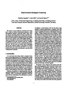
F IGURE 2.1: Overview of the main families of clustering algorithms for high dimensional datasets

The two first classes of this taxonomy are defined by the type of subspace produced by the algorithms. The third class constitutes a different category, since the way objects and features are considered is very different from the two previous classes. The diagram presented in Figure 2.1 represents the major families of approaches developed to overcome the curse of dimensionality and tackle the clustering problem in high dimensional spaces. In the next subsections we present the main families of subspace clustering algorithms, namely axis-parallel clustering, arbitrary oriented clustering and pattern-based clustering. At the end of this section we also provide a quick overview of other related approaches proposed to overcome the curse of dimensionality. Then in Section 2.3 we focus with more details on axis-parallel clustering, that is the family to which belong the algorithms developed in this thesis.

2.2.2

Axis-Parallel Subspace Clustering

The algorithms belonging to the axis-parallel clustering family look for clusters in subspaces that are subsets of the original features. In this case the subspaces are termed "axis-parallel subspaces". Historically two different terms have been used in parallel to evoke axis-parallel algorithms: subspace clustering and projected clustering. The former term was introduced in 1998 by Agrawal et al. [15], while the latter term was introduced one year after by Aggarwal et al. [13]. In principle, projected clustering algorithms ensure that the clusters produced are not overlapping (clusters are disjoint sets of objects) while subspace clustering algorithms allow clusters to overlap and a same object can belong to different clusters in different subspaces. Moreover subspace clustering aims at identifying all possible subspace clusters. To do so it uses a pruning criterion proposed first in the context of the mining of frequent itemsets in [14] and subsequently adapted to subspace clustering in [15]. This criterion is based on a monotonicity property that states that each cluster is defined in a given subspace is also defined in any lower dimensional projection of this subspace. Conversely, if a set of objects does not form a cluster in a given

2.2. Clustering in High Dimensional Spaces

13

subspace, it will not form a cluster in any higher dimensional subspace generated by adding dimensions to the initial one. In practice, the outputs of these two families are very similar and different hybrid methods have been proposed in the literature. In addition these two terms are not used consistently and projected clustering techniques usually refer to themselves as subspace clustering approaches. Moreover, subspace clustering has been used in the literature in a broader sense to denote different approaches even beyond the context of axis-parallel clustering. So in this thesis, to avoid ambiguities we refer to the subspace clustering approaches stemming from [15] as exhaustive subspace clustering. In addition to the historical differences between the terms presented previously, different taxonomies for axis-parallel approaches have been presented in the literature (e.g., [111] and [157]). These classifications are based on different concepts and present complementary points of view on the axis-parallel family. In Section 2.3.1 we describe the main taxonomies and we present the classification finally retained in this thesis.

2.2.3

Arbitrarily Oriented Subspace Clustering

Unlike axis-parallel clustering that defines subspaces only as subsets of the original features, the approach known as arbitrary-oriented clustering or simply oriented clustering defines subspaces as arbitrary oriented hyperplanes. Therefore this technique is more general than axis-parallel clustering in terms of spatial representation and for this reason arbitrary oriented clustering has also been called generalized subspace clustering or generalized projected clustering. Moreover arbitrary oriented clustering can express and represent complex positive and negative correlation between different features. Hyperplanes where these complex behaviours hold are usually described by means of linear dependencies between the different features, which denote linear correlations between those features. In this case arbitrary oriented clustering has also been called correlation clustering and the cluster subspaces found by this method are also referred as correlation cluster hyperplanes. Clustering algorithms belonging to this family generally search subspaces that are arbitrary oriented hyperplanes where a set of data objects are densely packed (i.e., where a cluster lays). Most of the arbitrary-oriented clustering algorithms rely on the intra-cluster variance to compute the cluster subspaces. In this case, subspaces are usually chosen such that the variance (i.e., the spread) of the object coordinates along them is low and thus the subspaces retain descriptions that exhibit a high similarity between objects from the same cluster. On the contrary, the variance along the perpendicular subspaces is high and thus orthogonal subspaces contain descriptions that distinguish data objects belonging to the same cluster. In practice, most of the algorithms that have been proposed to tackle this problem rely on the local use of the feature reduction algorithm known as Principal Component Analysis (PCA) [102]. This algorithm is applied to local groups of objects in order to find the so-called principal components, i.e., a new set of vectors defining an uncorrelated orthogonal basis. Notice that the directions found are ranked according to the variance of the data objects coordinates along them (the first principal component having the largest possible variance). Once the PCA algorithm has been applied locally, the most promising directions are selected to define the cluster subspaces. The new

14

Chapter 2. Subspace Clustering and Evolutionary Approaches

subspaces can then be defined by means of a set of equations describing each new feature as a linear combination of the initial ones. Interestingly, this kind of description may prove valuable on its own, for instance it has been extended to encode quantitative and predictive models in [2]. Since the Principal Component Analysis is applied to local groups of objects, these methods rely on the so called locality assumption to find subspaces. This assumption, applied to the context of arbitrary oriented clustering, implies that it is possible to compute the subspace of a cluster using the neighborhood of the cluster center. Therefore according to this assumption using a subset of the cluster objects should be sufficient to compute the subspace of the cluster. The first algorithm proposed to tackle the oriented clustering problem for arbitrary oriented disjoint clusters is ORCLUS [10]. This algorithm extends the axis-parallel clustering algorithm called PROCLUS presented in [13] that searches hyper-spherical shaped clusters. A variant of ORCLUS was proposed in [43] for multidimensional indexing. More recent approaches have also been proposed, for instance a variant of this algorithm that is resistant to noise and relies on Singular Value Decomposition (e.g., [75]) has been proposed in [126]. The first density-based approach developed to tackle the oriented clustering problem, called 4C has been proposed in [34]. Two other density-based algorithms called COPAC and ERiC have been proposed in [7] and [5] respectively. Both methods use information of the structure of the Principal Components Analysis decomposition in order to reduce the runtimes and improve the results. This subspace clustering family has even been extended to find clusters exhibiting non-linear correlation by the algorithm called CURLER [206]. In addition to density-based approaches, the hierarchical paradigm has also been extended to arbitrary oriented clustering by the algorithm HiCO [4]. According to [111] the major drawback of techniques relying on Principal Component Analysis are their runtimes. While these techniques scale linearly or at most quadratically with respect to the number of objects, their time complexity is usually cubic with respect to the number of features in the space. In addition to techniques based on Principal Components Analysis, other approaches have been investigated. For instance a method called CASH, proposed in [6], relies on the Hough Transform to map the data objects into a so-called parameter space, where the algorithm does not require the locality assumption any longer to produce subspace clusters. The use of Fractal Dimensions for arbitrary projected clustering has also been investigate for instance in [27] and [73]. Interestingly the pattern-recognition community proposed approaches based on random sampling techniques that are related to arbitrary oriented clustering (e.g., [84], and [83]). Some techniques belonging to the pattern-based clustering or biclustering family share some similarities with the arbitrary-oriented approach. However according to [111], the approaches relying on pattern-based clustering or on biclustering intuitions do not tackle the same problems addressed by arbitrary-oriented approaches.

2.2.4

Pattern-Based Clustering

The main difference between the pattern-based clustering approach and those previously described is related to the similarity measure used to define clusters: While

2.2. Clustering in High Dimensional Spaces

15

axis-parallel clustering and arbitrary oriented clustering algorithms use mostly distance similarity measures (e.g., Euclidean distance or the Manhattan distance), pattern-based clustering approaches use similarity measures based on "common patterns" of the data objects in a given subspace. Moreover, pattern-based approaches also differ from the two previous paradigms since they usually consider interchangeably the objects and the features of the dataset. Therefore the similarity can correspond to a group of objects presenting a common pattern along a given set of features, or to a set of features exhibiting a common pattern with respect to a given set of objects, or even to both a common joint pattern of a subset of dimensions and a subset of objects. For this reason this approach is also known as biclustering, coclustering, two-mode clustering or two-way clustering. In this context, datasets are usually organized in a matrix, such that objects are represented by the matrix rows and features by the columns. Different survey articles have been dedicated to pattern-based clustering in the literature. For instance, we refer the reader to [141], [211], [202] and [99] for detailed presentations of this family. In [141] authors categorized pattern-based clustering algorithms in four categories, namely constant biclusters, biclusters with constant values on either columns or rows, biclusters with coherent values and biclusters with coherent evolution. Hereafter we present each one of these categories and we provide some examples of algorithms belonging to each of them. Constant biclusters This family of pattern-based algorithms looks for sets of objects and dimensions for which all the coordinates along the different dimensions of the given subspace are equal to the same value. According to [111] this leads to a very particular scenario. Indeed, since a constant bicluster has the same coordinates along each dimension of its subspace, it invariably lays on the bisecting line with unitary slope and zero intercept defined in its corresponding subspace, which corresponds to a very particular location. In order to deal with real world applications the algorithms usually rely on a more relaxed condition: a cluster is formed if the different values are not too far from the mean value. For instance a classical example of the relaxed version of this approach, based on the intra-cluster variance has been presented in [85]. Biclusters with constant values on either columns or rows The algorithms belonging to this family constitute a more relaxed version of the previous approach. Biclusters with constant values on columns are constituted by objects that must have the same coordinates along each dimension, however the coordinates can differ from one dimension to another. Conversely, biclusters with constant values on rows are constituted by features that should provide the same coordinate for each distinct object, but this coordinate value may differ from one object to another. In this case the clusters are located on the hyperplanes defined by the relevant features. The bio-informatics community has developed many application driven methods employing such biclustering approaches, especially to analyze gene expression data gather in microarrays. For instance in [72] authors presented a robust biclustering approach that was able to cluster microarray samples according to genes or vice versa. A probabilistic model based on biclusering was presented in [186] and was applied to

16

Chapter 2. Subspace Clustering and Evolutionary Approaches

genomic expression data. Moreover, in [191] authors use such a biclustering strategy taking advantage of Gibbs sampling to detect patterns in noisy data. Biclusters with coherent values The algorithms from this category are more general than the previous approaches. In this case biclusters contain values that exhibit a correlation between rows and columns. Each coordinate in such a bicluster can be computed by taking the mean of the bicluster coordinates, and adding an adjustment value depending on the feature along which the coordinate is measured and another adjustment related to the object to which it belongs. Consequently this approach searches for clusters that exhibit a very particular correlation between rows or columns. The clusters are described in hyperplanes that are parallel to the relevant features axes and have a rectilinear shape defined by linear equation with unitary slope and arbitrary intercept. Notice that negative correlations cannot be captured by this approach. The term biclustering was first used for this particular pattern-based clustering family, in the context of analysis of genes expression arrays [48]. This work focused on the extraction of a given number of biclusters with coherent values referred as δ-biclusters, i.e., subsets of features and objects having a mean squared residue lower than a given parameter δ. A stochastic variant of this previous approach called FLOC was presented in [222]. A related algorithm called MaPle was presented in [173], avoiding redundant biclusters and focusing only on maximal biclusters. k-means flavored biclustering algorithms for biclusters with coherent values have also been proposed, for instance in [50]. Biclusters with coherent evolution The algorithms belonging to this category look for biclusters that contain objects such that their coordinates have the same tendency when they are analyzed with respect to different features, e.g., if the coordinate of a given object is higher in a given feature than in another, then this should also happen for the other objects in the cluster. Some approaches only consider the direction of the change and not the value itself, while other approaches quantize the coordinates over continuous domains into discrete states and consider a change of discrete state from one feature to another, e.g. [158]. The approach presented in [28] introduces the concept of order-preserving submatrices, i.e., set of objects and features such that every feature induce the same tendency on the coordinates of the distinct objects. The same concept has been used in [130] to define a model called OP-Cluster (Order Preserving Cluster). This approach defines the similarity between two objects on a given subset of features as the capacity of the values of those objects to lead to a similar ordering of the features. As the three previous biclustering approaches, this category also has been applied to gene expression data. Graph oriented representations Regardless of the kind of biclustering approach that was addressed, different graph oriented representations for biclustering have been proposed in the literature. This approach has received an special attention in the context of binary data. In this case datasets have been represented as bipartite graphs connecting objects and features and the biclustering task corresponds to the search of bicliques in the bipartite graphs representing the dataset. For instance in [203] authors proposed a representation of gene expression data based on a weighted bipartite

2.2. Clustering in High Dimensional Spaces

17

graph between a set of nodes representing genes and a set of nodes representing biological situations, such that the weights on the edges represent the level of expression of the genes in each situation. Other approaches that have been proposed, rely on a more relaxed definition of biclustering based on quasi-bicliques. For instance in [199], authors have proposed a biclustering approach based on the search of quasi-bicliques in a bipartite graph to analyze stocks and financial ratios. Other approaches based on quasi-bicliques have also been proposed for instance in [198], [125], [150] and [195]. Similarly, in [56] authors proposed a representation of a document collection as a bipartite graph between words and documents along with spectral graph partitioning. More generally biclustering methods based on graph oriented representations have also been proposed to deal with matrices of occurrences, in this case bi-clusters are usually called co-clusters and the pattern-based clustering task is commonly referred as co-clustering. Another co-clustering method based on graph partitioning was proposed for instance in [179]. Other approaches relying on a graph representation and mutual information to perform co-clustering were proposed for instance in [57], [197], [71] and [49].

2.2.5

Other related Tasks

Besides subspace clustering algorithms, other related approaches have been proposed to overcome the curse of dimensionality and cluster high dimensional data. An intuitive idea that has been explored is to reduce the dimensionality of the dataset, for instance by removing irrelevant features, and subsequently apply traditional clustering algorithms in a lower dimensional space. The approaches based on this idea, rely for instance on techniques such as features selection (e.g. [55]) or features reduction (e.g. [58]) to reduce the dataset dimensionality before applying traditional clustering techniques. Furthermore a different approach called soft-projected clustering aims to deal with high-dimensional spaces by associating a weight to each feature. 2.2.5.1

Feature Selection and Feature Reduction

According to [111] a classical way to deal with high dimensional data consists in applying methods known as feature selection or features reduction before applying mining algorithms per se. This first step allows to project the entire dataset into a new space (or a subspace) with lower dimensionality. Since classic distance measures are likely to be more meaningful in the lower dimensional space, traditional data mining algorithms are then likely to produce more promising results in this new space. Two major families of global dimensionality reduction exist: feature selection and feature reduction. Both approaches are described hereafter. Feature selection Feature selection is a data mining task used to select only a subset of the original features, removing irrelevant and redundant attributes from the dataset. This task is usually applied with other data mining techniques such as clustering, classification or regression. When this technique is used before applying a clustering algorithm, the features that are selected are those along which the objects are well clustered.

18

Chapter 2. Subspace Clustering and Evolutionary Approaches

The feature selection task is somehow analogous to the axis-parallel clustering approach presented in Section 2.2.2. Indeed the feature selection approach applies a global dimensionality reduction by selecting a promising subset of the features and the axisparallel clustering task applies the same kind of dimensionality reduction locally to each cluster in order to find adequate subspace for each cluster. Notice that this technique does not apply a transformation to the original features, it only extracts the projection of the data objects along the selected features. Two major approaches exist and are called the wrapping model and filter model. The algorithms that follow the principles of the filter model are independent from the clustering task since they select a set of features according to some predefined criteria and apply the clustering afterwards. For instance an example of this approach can be found in [55]. In the wrapping model, the clustering algorithm is used iteratively by the feature selection technique to evaluate the quality of the set of dimensions that are being selected by the algorithm. Then the best set of dimensions found by the algorithm is chosen and finally the clustering algorithm is applied to the projected dataset to produce a clustering model. An example of this technique can be found in [106]. Feature reduction Unlike feature selection, the feature reduction approach does not only select a subset of features to reduce the dimensionality of the dataset. This technique performs a linear and even a non-linear mapping of the dataset to a lowerdimensional space. Hence, the coordinates of an object in the new space can be expressed as a combination of the original coordinates of the given object. Notice that the feature reduction task is somehow related to the arbitrary-oriented clustering approach presented in Section 2.2.3. Indeed the feature reduction approach apply a global dimensionality reduction based on a linear or even a non-linear mapping of the dataset, and arbitrary-oriented clustering apply a similar dimensionality reduction locally to each cluster in order to find an adequate subspace for each cluster. This approach is interesting since it does not constrain the cluster to subspaces of the original features, and allows to construct new subspaces (e.g., by linear combination of some original features). A common approach consists in applying linear feature reduction using algorithms such as the Principal Component Analysis (PCA) [102] or the Singular Value Decomposition (SVD) [75]. In this case the new features are expressed as a linear combination of the original features. Some approaches also involve non-linear transformations that map the feature space in a lower dimensional space in such a way that nearby objects are mapped close to each other (e.g. [140] and [181]) Different clustering algorithms for high dimensional datasets relying on feature reduction have been proposed in the literature. An example of this approach can be found in [58] for instance. Notice that some techniques of feature reduction are considered sensitive to noise and that the meaning of new features is sometimes difficult to interpret. The major drawback of these two approaches is that the reduction of the dimensionality is global. Consequently if a particular group of points is well characterized in a subset of dimensions, while a different group of points is better described in a different subspace, then this information is not taken into account. Indeed, different subsets of features could be relevant for different clusters, this phenomenon is known

2.3. Focusing on Axis-Parallel Subspace Clustering

19

as local features relevance or local features correlation [111]. Depending on the dataset and also depending in the task, the local features relevance for each particular cluster can be important and applying a global dimensionality reduction may lead to the loss of this information, and even in some cases to the loss of the cluster structures themselves. Therefore, if the task requires to capture the local features relevance, a global feature selection should not be applied. 2.2.5.2

Soft-Projected Clustering

A different approach called soft-projected clustering has also been proposed in the literature to find clusters in high dimensional spaces. This technique deals with highdimensional data by assessing the importance of each feature for each one of the existing clusters using a system of weights. These weights facilitate the adaptation of the shape of the different clusters to each dimension. Different approaches derived from the well known k-means algorithm have been developed for soft-projected clustering (e.g., [59] and [47]). Another algorithm presented in [70] relies on the computation of a similarity matrix instead. Even if the relative importance of the different features are evaluated differently for each cluster, the different clusters are always expressed in the full space and the relevant dimensions for each cluster are never explicitly selected. This element differentiates soft-projected clustering from subspace clustering. We refer the reader to survey articles on soft-projected clustering for a thorough presentation of this technique (e.g., [100], [37] and [218]).

2.3 2.3.1

Focusing on Axis-Parallel Subspace Clustering Classification of the Axis-Parallel Approaches

Among the different subspace clustering families presented in the previous section, the axis-parallel clustering family is an important category that aims at finding clusters in subspaces that are defined as subsets of the original features. Since the algorithms presented in this thesis belong to this family, more details regarding this category are given hereafter. In this section we present different taxonomies used in the literature to classify axis-parallel clustering algorithms. 2.3.1.1

Algorithmic-oriented categorization

In [171] the authors proposed a classification of the existing approaches that was based on their respective algorithmic strategies. This categorization has been called algorithmic-oriented categorization in [111]. Two major strategies have been identified: the top-down and the bottom-up ones. Top-down approaches Most top-down algorithms start from a clustering in the full dimensional space and use the locality assumption to find the cluster subspaces. According to this assumption the neighborhood of the cluster center is representative enough of the whole cluster, and it is possible to determine the subspace of the cluster using only this neighborhood. Other methods are based on random sampling to

20

Chapter 2. Subspace Clustering and Evolutionary Approaches

produce the subspaces of previously found clusters. Since top-down approaches start from clusters expressed in the full space and then compute their respective subspaces reducing their dimensionality, these methods are also known as dimension-reduction subspace clustering. Bottom-up approaches The principle of this approach is to find all the promising one-dimensional subspaces (that contain clusters), and then to combine them in order to build subspaces with higher dimensionalities. This family of methods is based on the assumption that if a cluster is defined in a given subspace, then it also exists in any subset of dimensions taken from its subspace. Since these methods start with simple one-dimensional clusters and then combine them to produce clusters laying in subspaces with higher dimensionalities, these methods are also known as dimensiongrowth subspace clustering. The algorithmic-oriented categorization provides an interesting taxonomy based on the algorithmic approach used to tackle the subspace clustering problem, i.e., the assumptions and the strategies used to build subspace clusters. However the same algorithmic approach (top-down or bottom-up) can be used to produce very different clustering models depending on the similarity measure and the underlying definition of subspace clusters. 2.3.1.2

Problem-Oriented Categorization

In addition to the algorithmic oriented categorization, in [111] the authors presented another criterion called problem-oriented categorization. In this taxonomy the algorithms are classified according to the problem or the task they tackle. Four classes of problems have been distinguished in [111], corresponding to the following clustering categories: • The first one corresponds to the soft projected clustering approach that has been presented in Section 2.2.5.2. The algorithms belonging to this family seek a specific number of clusters using a weighted contribution for every dimensions in the dataset. • The second category is called the projected clustering approach (introduced in Section 2.2.2). The algorithms belonging to this family produce a crisp clustering model, since they assign each object to a unique cluster, and they assign to each cluster a unique subspace. • The third category (presented also in Section 2.2.2) that was presented is the exhaustive subspace clustering approach. The algorithms belonging to this family may assign the same data object to different subspace clusters, unlike projected clustering approach. Moreover they aim at identifying all possible subspace clusters (i.e., they try to find all the subspaces where a cluster can be identified) and consequently they usually produce a large number of subspace clusters. • The last class gathers the so-called hybrid algorithms that are in between the exhaustive subspace clustering approach and the projected clustering approach. Unlike projected clustering, these algorithms allow clusters to overlap and contrary to subspace clustering algorithms, they do not provide all clusters in all subspaces.

2.3. Focusing on Axis-Parallel Subspace Clustering

21

The problem-oriented categorization provides an interesting classification based on some underlying definitions of clusters (problem statement). Moreover the problemoriented categorization and the algorithmic-oriented categorization are related to each other, since many algorithms belonging to the projected clustering family are based on a topdown technique while most of the exhaustive subspace clustering algorithms belong to the bottom-up approach. 2.3.1.3

Categorization based on traditional clustering families

In [157] authors have presented a different categorization for axis-parallel algorithms. This taxonomy, as well as many classifications made for traditional clustering approaches (e.g., [95], [29]), is based on the underlying clustering paradigms and definitions that the algorithms assume. More precisely, three main families have been identified and categorized in [157] • The first category corresponds to the so-called clustering-oriented family (also called partitioning relocation clustering in the context of traditional clustering (e.g., [29])). The algorithms belonging to this category are based on the representation of clusters by means of a set of prototypes and the association of the data objects to their most similar prototype. These approaches are usually expressed as the optimization of a global criterion that measures the adequacy between the data objects and the prototypes. For example, in the context of traditional clustering approaches, the well known k-means algorithm that aims to optimize the sum of square of euclidean distances between each objects and its closest centroid, falls in this category. This family contains also the well known k-medians and k-medoids methods as well as different probabilistic approaches. • The second family is the density-based category. The algorithms that follow the density-based paradigm do not represent clusters using prototypes and do not rely on a global optimization procedure. Instead, these approaches are based on local optimization criteria that analyze the local structure of the data to find dense regions in the datasets. For example, in the context of traditional clustering, the well known DBSCAN algorithm falls in this category since it uses the local structure of the dataset to detect locally dense regions and then connect them to form arbitrary shaped clusters. • The third category has been termed cell-based family (the term grid-based family can also be found in the literature). As well as in the previous family, cell-based approaches rely on a local exploration of the dataset to find regions containing densely packed data objects. In this case explorations are also based on local optimization criteria. The main difference between the approaches belonging respectively to the density-based family and the cell-based one is that the former detect dense spherical shaped regions around data objects and then connect them to form clusters, while the latter relies on a discretization of the space using a grid, detect dense cells and connect neighboring dense cells to build clusters. Notice that the differences between these two families have also been brought up in the context of traditional clustering algorithms to distinguish two important categories of algorithms (e.g., [29]).

22

Chapter 2. Subspace Clustering and Evolutionary Approaches

These different approaches are complementary tools that allow the users to analyze data from different perspectives. In the next sections we used this taxonomy to present the different axis-parallel approaches from the literature, since it is based on the underlying clustering paradigm used by the algorithms, which is a very important concept that defines the kinds of clusters produced.

2.3.2

Cell-Based Approaches

The cell-based or grid-based clustering family is based on the optimization of local criteria and its main characteristic is related to the previous partitioning of the dataset using a grid structure. More precisely, most cell-based clustering algorithms first use a grid structure and distribute the data objects in cells, then the cell densities are computed, all dense cells are selected and aggregated locally to form the final clusters. This method is based on the local optimization of the density of cells and also on the expansion of dense cells to form clusters. CLIQUE [15] is the first algorithm that extended this paradigm to subspace clustering. This algorithm is a typical example of the cell-based clustering family. In CLIQUE, clusters are defined as connected hyper-rectangles laying in specific subspaces and containing more than a given number of objects. Initially, the algorithm partitions each feature into a fixed number of cells laying in one dimensional subspaces, the size and the number of cells are parameters of the algorithm. Then the algorithm uses a bottom-up approach to intersect these cells into cells laying in higher dimensional axis-parallel subspaces. Then CLIQUE selects cells that contain more objects than a threshold given as a parameter and builds clusters by aggregating dense cells that are adjacent (connected to each other). Since setting the size or the number of the cells and the density threshold may result in a delicate task, possibly leading to poor clustering, some authors came up with adaptive grids. For instance the algorithm called MAFIA [160] and its parallel version pMAFIA [161] have been proposed to overcome these difficulties. Another adaptive algorithm called DOC has been proposed in [177]. This algorithm initially uses data object samples as seeds to build flexible hypercubes described in axis-parallel subspaces. Then the given hypercubes are updated with respect to a parameter specifying the trade-off between the number of points in the hypercubes and their respective dimensionality. It has been suggested that the use of this parameter may lead DOC to encounter problems while dealing with clusters with very different subspace dimensionalities. A more recent version of DOC called MINECLUS has been proposed in [224]. This algorithm uses a more efficient representation based on frequent pattern tree (FP-trees) and has expressed the subspace clustering problem as a frequent itemset problem. As a result the MINECLUST algorithm exhibits lower runtimes than its predecessor DOC. A different algorithm called SCHISM, presented in [188] also extends the cell-based paradigm using flexible thresholds adapted to the dimensionality of the subspaces in order to mine only interesting subspaces rather than all the possible subspace clusters directly. Another algorithm called ENCLUS, presented in [46], is also a grid-based algorithm that relies on an entropy measure to prune subspaces and filter out irrelevant subspaces.

2.3. Focusing on Axis-Parallel Subspace Clustering

23

An interesting algorithm called nCluster presented in [128] and [129] has introduced a variant of the grid-based family based on distance measures that aims to overcome weaknesses of the grid-based approach related to the possible inappropriate partitioning of the dataset using grids. This problem can be sketched with a simple example: let us imagine a dense group of points that could be placed in one cell to form a cluster, now let us imagine this group is in fact spread over two cells, and that the number of objects in each cell is not sufficient to form two contiguous dense cells. In this case this dense group of points does not form a cluster and is lost. To overcome this problem, nCluster allows for overlapping cells and scans the dataset using a window that slides in the data space seeking for clusters. In [196], authors present this approach as belonging to a specific clustering family that they called window-based clustering. Recent approaches have extended the cell-based paradigm to more complicated tasks. For instance the algorithm called HSM [156] is an extension of CLIQUE for heterogeneous data, i.e., data containing both categorical and continuous features.

2.3.3

Density-Based Approaches

The density-based clustering family is also based on the optimization of local criteria. The algorithms belonging to this family extend to subspace clustering the principles proposed in the pioneering algorithm called DBSCAN [61]. Density-based clustering algorithms are based on the underlying definition of clusters as dense groups of objects that can be arbitrarily shaped but must be separated from each other by regions with low density of objects. In practice, most of the density-based algorithms start by computing, for each data object, the number of neighbors within a sphere of a given radius. Then, they usually select dense regions, i.e., regions containing more objects than a given threshold within a given radius. Finally clusters are built by joining together the objects from adjacent dense regions. Notice that the sphere radius, the distance measure and the density threshold are very important parameters for this family of algorithms. The first extension of DBSCAN for subspace clustering, called SUBCLU, has been presented in [116]. This algorithm is based on a bottom-up approach that starts applying DBSCAN along each feature independently and then build clusters in higher dimensional subspaces gradually. Since the scanning of the neighborhood of each data object is an expensive task, an algorithm relying on approximate solutions called FIRES has been proposed in [110]. FIRES is a bottom-up algorithm that uses the information of histograms over each feature to mine higher dimensional clusters by merging clusters having many intersecting objects. The aggregation is different from most bottom-up algorithms and aims to scale at most quadratically with respect to the dimensionality of the dataset. This algorithm also uses a post-processing step that prunes and refines the clusters in a topdown manner. In order to limit problems related to poor setting of the neighborhood radius parameter, FIRES also employs a strategy that adapts the radius with respect to the cluster subspaces. The authors of [20] presented INSCY a density-based algorithm that does not follow a bottom-up technique as the two previous algorithms. INSCY is based on a depth-first search processing that prunes lower dimensional subspaces recursively

24

Chapter 2. Subspace Clustering and Evolutionary Approaches

from already detected higher dimensional subspace clusters. This algorithm proposes a method to adapt the density threshold to the subspace dimensionalities keeping a fixed radius parameter. The previous approaches have came up with different techniques to adapt some of the parameters such as the radius or the density threshold to be more flexible when dealing with clusters with different subspace dimensionalities. However these techniques are still highly dependent on the distance measure used to compute the similarity between data objects and thus they are still subject to the classical problem of distances in high dimensional datasets known as the curse of dimensionality. To overcome such problems different works have been proposed. For instance an algorithm called DUSC, presented in [19], uses a distance measure that adapts to the size of the subspace clusters that are analyzed. Similarly the subspace clustering algorithm called PreDeCon, proposed in [35], extends the DBSCAN algorithm using a weighted Euclidean distance. Finally, notice that the density-based subspace clustering family also includes hierarchical approaches, as DiSH [3] (inspired on OPTICS [18]) or HARPS [223].

2.3.4

Clustering-Oriented Approaches

The clustering-oriented approaches are based on the optimization of global criteria. The algorithms belonging to this family usually represent clusters by means of some prototype and associate objects to their best prototype. In addition to a dedicated definition of the notion of cluster prototype, the algorithms are based on parameters specifying properties of the targeted clustering such as the expected number of clusters or the cluster average dimensionality. According to these constraints, the objects are grouped together usually using distance-based similarities, in order to match the closest prototype, optimizing a global criterion reflecting the quality of the subspace clustering model. Interestingly many of these methods tend to build center-based hyper-spherical shaped clusters. PROCLUS presented in [13] is the first algorithm that extended this paradigm to subspace clustering. Its main parameters are the number of clusters and their average dimensionalities. This algorithm is to some extent an extension of the well-known traditional clustering task known as k-medoids. Indeed, this algorithm uses data objects themselves as prototypes for the clusters (i.e., cluster medoids). Then data objects are assigned to their closest medoid using a distance measure that is adapted to subspace clustering task. More precisely, the distance between an object and a medoid is measured in the cluster subspace using a variant of the Manhattan distance, called the Manhattan Segmental Distance. This distance normalizes the usual Manhattan distance by the dimensionality of the subspace where the distance is measured. The subspace of each cluster is produced by selecting the dimensions along which the dispersion of data objects is low in the cluster. PROCLUS also includes a post-processing step consisting in an outlier detection procedure and a subspace refinement heuristic. This algorithm outputs spherical shaped clusters grouped around medoids and each cluster is described in its own subspace. FINDIT [221] is a variation of PROCLUS that uses more heuristics to enhance the results.

2.4. A Challenge: Clustering and Subspace Clustering of Data Streams

25

A different algorithm based on a statistical description of clusters called P3C has been proposed in [153]. This algorithm relies on statistical chi-squared tests and Expectation-Maximization optimization to partition the dataset and find subspaces. P3C is a bottom-up algorithm that starts with one-dimensional intervals that contain dense regions and merges them in order to produce clusters defined in higher dimensional subspaces. P3C relies on the Mahalanobis distance as similarity measure. Moreover, P3C aims at being a robust algorithm able to find the true number of hidden clusters in the dataset and to detect clusters with low dimensional subspaces in high dimensional datasets. A more recent algorithm that also relies on a statistical description of clusters and statistical methods to extract subspace clusters, called STATPC, has been proposed in [152]. This algorithm formulates the subspace clustering task as an optimization problem that aims at finding clusters that exhibit a statistical significant density.

2.4 2.4.1

A Challenge: Clustering and Subspace Clustering of Data Streams Introduction

Clustering of data streams is a task that has been actively addressed by the data mining community. Important application domains such as network monitoring, sensor networks, meteorological analysis and stock market analysis require the use of data mining and clustering algorithms specially designed to deal with possibly infinite streams of data. Data streams specificities Traditional clustering algorithms are not directly adapted to deal with data streams. Since the entire data stream usually cannot be stored (bounded memory), the algorithms cannot run several passes over the possibly infinite dataset (single pass). In addition, the notion of stream also often implies that the system needs to deal with the data in real time, so the clustering algorithms for data streams should provide an accurate model in a single pass, anytime and fast enough in order to follow the stream in real time. Moreover in many applications the data streams are likely to evolve dynamically: underlying clusters can appear, disappear, move in the space and their relative importance along each dimension can change. Consequently data stream clustering algorithms should be able to follow such changes dynamically and keep the clustering model up to date by incorporating into the model new information received and removing the effect of outdated objects from the clustering model. Types of data streams Data streams have been categorized in two classes in [196]. The first class of data streams has an infinite number of objects arriving at different time stamps. The second class of data streams is constituted by a given set of object but having attribute values that change over time. Some algorithms have been proposed to deal with this latter case, for instance in [107] authors developed a special cell-based approach allowing overlapping cells using a window that slides in the feature space.

26

Chapter 2. Subspace Clustering and Evolutionary Approaches

However in this thesis we focus only on the first class of data streams, the ones made of a stream of new objects arriving over time. Window model The algorithms that have been proposed in the literature use different approaches to address the temporal changes of the data streams. The temporal aspect of the data stream is addressed by defining a window model used to analyze the stream. Some applications may focus on the entire data stream from the beginning without prioritizing more recent objects. This approach, known as the landmark window may be incompatible with the idea of analyzing an evolving data stream, since in this case the resulting model would be dominated by outdated data. A different approach known as sliding window only focus on the most recent objects. The number of objects considered (the window length) is usually an important parameter since a large window presents the same drawbacks of the landmark window, while small windows with only few points are not representative of the dataset and may lead to poor results. Another variant called fading window assigns a weight to each data object according to the timestamp of its arrival, and the weights of old points tend to fade exponentially. This approach relies on a fading parameter that defined the speed of fading. Finally the so-called tilted time window uses different levels of granularity in order to keep a more global picture of the data stream. This approach usually assigns a fine scale to recent data and a coarse one to old ones. Algorithmic approaches Independently from the temporal conception used by the different algorithms to deal with data streams, two major algorithmic approaches have been proposed. The approach called incremental learning aims at updating incrementally the clustering model to take into account the changes in the data stream. The update can be achieved when a new object arrives or when the window changes. With this approach the user can directly access the updated model. Unlike the incremental learning approach, the two-phase learning or online-offline approach does not keep a model constantly up to date. Instead this approach splits the clustering task in two stages: an online stage updates and stores a summary of the data stream in real time while an offline stage performs a clustering over the summary whenever the user requires a clustering model. Clustering paradigms The major clustering families have been extended in order to deal with data streams using different algorithmic approaches and different kinds of temporal window models. In addition, a few approaches of subspace clustering have also been extended to data stream analysis, namely the clustering-oriented, densitybased, cell-based and hierarchical clustering families. In the section hereafter we present some extensions of the major clustering families to the analysis of data streams. Since the different algorithms developed in this thesis belong to the clustering-based approach we will focus our description on this family. For a thorough presentation of the different clustering algorithms for data streams the reader is referred for instance to the following survey articles [8], [162] and [194].

2.4. A Challenge: Clustering and Subspace Clustering of Data Streams

2.4.2

27

Clustering-oriented approach

Different algorithms that extend the clustering-oriented approach to data streams analysis are based on the well-known k-means or the k-medians algorithms. For instance one of the first of these algorithms, the STREAM algorithm, presented in [76] and enhanced in [164], extends the k-medians algorithm. This algorithm splits a dataset into chunks that are processed separately to produce clusters. When the number of clusters stored exceeds a given threshold, the weighted centers of the clusters found are themselves processed to form cluster of cluster centers, and so on. Since the algorithm stores clusters for each chunk and then agglomerates clusters, it can be considered as based on a tilted time window technique. Another approach called CluStream presented in [11] is a two-phase learning approach, based in two separate components. The first stage performs an online microclustering stage that processes a data stream in real time and only keeps an abstract summary statistics made of microclusters. The second is an offline macro-clustering algorithm that runs over the abstract description made of the micro-clusters. The CluStream algorithm also relies on a tilted time window technique since it stores the micro-clusters at different time scales following a so-called pyramidal time frame to keep information at different horizons. An extension of this technique relying on a more efficient data structure to store micro-clusters was proposed in [109]. The user can execute the macro-clustering algorithm at different temporal horizons whenever it is required. Since the macro-clustering technique used is an extension of the k-means algorithm, this approach belongs to the clustering-oriented approach. It is interesting to notice that the pyramidal storage of micro-clusters has also lead some authors to categorize this approach as a member of the hierarchical clustering family. In [226] authors affirm that pyramidal micro-clustering storage used in CluStream is likely to be inefficient to deal with data clusters shifting in space. Authors propose SWClustering a two-phase learning that builds and maintains micro-clusters using a sliding window approach. The macro-clustering stage is also based on k-means and thus this algorithm also belongs to the clustering-oriented family. Another two-phase learning algorithm called E-stream has been proposed in [207]. This algorithm uses a fading window representation and special procedures that allow the algorithm to follow cluster appearance, disappearance, merge, split and selfevolution. HUE-stream, an extension of E-stream for heterogeneous and uncertain data has been presented in [148]. It is interesting to notice the use of the terms "evolution-based" or "evolving" to denote algorithms designed to tackle clustering of data streams, these terms refer to the evolving character of the data stream and not to the algorithm itself (i.e., they are not evolutionary algorithms).

2.4.3

Density-based stream clustering

Different techniques of data stream clustering belonging to the density-based family have been proposed in the literature, here we focus on two well-known approaches called DenStream and OPTICS-Stream. The two-phase learning algorithm called DenStream, proposed in [38], extends the density-based approach using a description of the stream based on weighted microclusters. This algorithm is based on a fading window temporal paradigm and thus the

28

Chapter 2. Subspace Clustering and Evolutionary Approaches

weight of each micro-cluster is computed according to a fading function such that old objects have a low weight and are less important for the clustering task. As most density-based approaches, this algorithm aims at detecting dense regions called here core micro-clusters. Micro-clusters that are not dense enough to be core micro-cluster are labeled as potential core micro-clusters or even outlier micro-clusters if their corresponding weight is too low. When a new object arrives, the algorithm preferentially attaches it to its closest core micro-clusters or potential core micro-clusters, if the data object is too far away from them (beyond a given threshold) the algorithm tries to attach it to the closest outlier micro-cluster, if once again the closest outlier micro-cluster is too far from the object, the algorithm creates a new outlier micro-cluster containing the object. The algorithm maintains micro-clusters dynamically and uses DBSCAN as an offline algorithm to group the micro-clusters in arbitrary shaped dense regions of connected dense micro-clusters when the user requires a clustering model. Similarly, the two-phase learning algorithm OPTICS-Stream presented in [204] relies on micro-clusters and a fading window approach to produce an online summary of the data stream and computes a macro-clustering using the density-based algorithm OPTICS under request.

2.4.4

Cell-based stream clustering

Cell-based approaches and density based approaches are very similar conceptually. The algorithm called D-Stream proposed in [45], extends the cell-based clustering family to the data stream context. This algorithm is similar to a density-based algorithm but it relies on a cell-based discretization of the space instead of using micro-clusters. Similarly to DenStream [38], each object is characterized by a weight that decays exponentially with time (fading window). Analogous concepts to core micro-clusters, potential core micro-clusters and outlier micro-clusters used in [38] are also defined for the grids used in [45]: dense grid cells, transitional grid cells and sparse grid cells. Cells are maintained by the algorithm incrementally and an offline algorithm can be executed anytime to form large dense regions by grouping adjacent dense grid cells. An extension of the D-Stream algorithm called DD-Stream has been proposed in [98]. A different approach called Statsgrid extending the hierarchical clustering paradigm on a cell-based manner was presented in [170] and subsequently extended in [168] under the name CellTree. The MR-Stream algorithm proposed in [217] also extends the hierarchical clustering paradigm using a cell-based representation. This algorithm is also a two-phase learning algorithm and relies on a fading window temporal structure.

2.4.5

Other stream clustering families

In addition to some grid-based algorithms that also extend the hierarchical family (e.g., MR-Stream and CellTree) other algorithms have been proposed to extend the hierarchical approach. For instance a hierarchical graph-based clustering algorithm for data streams called RepStream has been presented in [138]. This algorithm represents each data object as a graph node and each node is connected to its k-nearest neighbors. Then the algorithm uses the connectivity of each node to select representative objects and updates the connectivity when new objects arrive. This algorithm also uses the

2.4. A Challenge: Clustering and Subspace Clustering of Data Streams

29

fading window temporal representation to avoid a model biased towards outdated data and prune old data objects and non-representative ones to reduce the memory usage.

2.4.6

Subspace Clustering of Data Streams

It is common that the objects that arrive in a data stream are described by a large number of dimensions. In this case the problem known as the curse of dimensionality also leads the traditional clustering algorithms for data stream to struggle. To deal with this problem, subspace clustering algorithms have been extended to the analysis of streams of data. In this section we will focus on the approaches belonging to the axis-parallel clustering family (the same one to which belong the approaches developed in this thesis) and we follow the same taxonomy presented in Section 2.3, i.e., the density-based, the cell-based and the clustering-oriented families. 2.4.6.1

Density-based approach

The subspace clustering family that received more attention in the context of data streams is the density-based one. In [113] and [114] authors proposed an incremental version of the density-based subspace clustering algorithm called PreDeCon [35]. Subsequently this algorithm was extended to subspace clustering of data streams in [86], this algorithm is called PreDeConStream. Another density-based subspace clustering algorithm called HDD-Stream has been presented independently in [163] and also extends the PreDeCon algorithm to data streams. The algorithms presented previously use an exponential fading window in order to deal with the temporality of the data stream. These algorithms also belong to the two-phase learning family: micro-clusters are produced and maintained to summarize the data stream and the PreDeCon algorithm is used offline to produce macro-clusters. The micro-clustering maintenance technique is similar to the one presented in Section 2.4.3 for the DenStream algorithm. 2.4.6.2

Cell-based approach

The first algorithm that extended the cell-based approach to subspace clustering of data stream is GCHDS [134]. This algorithm uses a fading window to avoid the impact of outdated data and belongs to family of two-phase learning algorithms. The first phase stores a set of dense cells and maintains it iteratively. Whenever a clustering model is required, the second phase of the algorithm produces the clusters subspaces by selecting the dimensions along which the object coordinates are not distributed uniformly. Then,it aggregates cells that are not dense enough to reduce the number of clusters produced. In [169] the authors presented the Sibling Tree algorithm, a cell-based subspace clustering algorithm for data streams. This work extends two previous algorithms for clustering data streams presented in [168] and [170]. This algorithm monitors each feature with a list of cells called sibling list in order to find dense cells. Then a second level of lists monitors dense grids (clusters) in two dimensional subspaces. Successively, additional lists are used to monitor higher dimensional cells. The algorithm relies on a fading window in order to deal with the temporal aspect of the stream and proceeds to update the final clustering model in an incremental manner.

30

Chapter 2. Subspace Clustering and Evolutionary Approaches

A similar approach called Haliteds has been proposed recently in [193]. This algorithm extends the subspace clustering algorithm for static data presented in [53] and relies on a two-phase learning principle and a sliding window. 2.4.6.3

Clustering-oriented approach

The first algorithm that extended the clustering-based approach (center-based), called HPStream, was presented in [12]. This algorithm follows an incremental learning technique, it constructs and maintains a set of fading cluster structures. The algorithm is based on a fading window and each object has a weight that decreases exponentially with time. Two major parameters are required: the number of clusters k and the average dimensionality of the clusters l. Each cluster is characterized by four elements: the weighted sum of squares of the cluster object coordinates along each dimension, the linear sum of the cluster object coordinates along each dimension, the sum of the weights of the cluster objects and a binary vector that encodes the relevant dimensions for the cluster. Using this information it is possible to compute the location of the cluster center and the intra-cluster variance. For each cluster, the algorithm computes the variance along each dimension and finally the l × k dimensions leading to the lowest intra-cluster variance are chosen as relevant dimensions. The algorithm requires to be initialized by executing the k-means algorithm over an initial data sample and by selecting the most promising dimensions. Then, the algorithm updates incrementally the clusters each time a new object arrives: it assigns the new object to the closest cluster only if the object is within a given radius away from the cluster. Otherwise a new cluster is created and the oldest cluster is deleted in order to keep a constant number of clusters. At each time step the clusters having an empty subspace are erased from the model. More recently a very similar algorithm called SE-Stream has been presented in [41], [216] and [42]. This algorithm also relies on a fading window to deal with outdated data and stores fading cluster structures similar to the ones used by HPStream. In addition to the information stored in HPStream fading clusters, SE-Stream also stores for each cluster, along each dimension, a histogram to represent the distribution of the data. Based on these histograms, the algorithm uses special operators to merge clusters that are overlapping and split single clusters that contain sparse regions. Thanks to these operators, this algorithm aims to be more reactive than HPStream and thus authors define their approach as "evolution-based" (notice however that SE-Stream is not an evolutionary algorithm). This technique has been compared to the state-of-the-art technique HPStream only on two real world datasets and using only two evaluation measures and present slightly better results but higher runtimes [41]. In [87] and [88], authors proposed an interesting framework to produce subspace clustering models of data streams based on the two-phase learning principle. They proposed to combine existing online micro-clustering algorithms and offline subspace clustering algorithms. As in the other two-phase learning techniques, this approach uses any online algorithm to create and maintain data summaries using micro-clusters, then whenever the user requests a macro-clustering model, the micro-clusters are used to reconstruct an approximation of the data objects assuming a Gaussian distribution

2.5. Evolutionary approaches for Clustering and Subspace Clustering

31

of the objects within a micro-cluster and then any offline subspace clustering can be executed on this approximated data set. However the results of such hybrid algorithms have not been compared to existing approaches and the validity of the approximate reconstruction of the dataset has not been studied.

2.5

Evolutionary approaches for Clustering and Subspace Clustering

In this thesis we aim at taking advantage of evolutionary algorithms based on evolvable genome structures and bio-inspired mutational operators to tackle the subspace clustering problem. Therefore, in this section we focus our attention on previous evolutionary approaches proposed for clustering, subspace clustering and clustering of data streams.

2.5.1

Introduction

Evolutionary algorithms are a family of optimization methods inspired by darwinian evolution. These approaches incorporate different bio-inspired mechanisms, such as mutation and recombination operators, reproduction and selection schemes, in order to evolve a population of candidate solutions to a specific optimization problem. These candidate solutions are also referred as individuals, and each individual is characterized by its genome, following the biological analogy. In practice the quality of each candidate solution is assessed using a fitness function. Then the different individuals undergo selection, i.e., they reproduce differentially according to their fitness value so that better individuals, characterized by a higher fitness, have more chances to reproduce. Hence, the population-based search is guided towards more promising solutions. The reproduction of the best individuals consist in copying the parental organism and then applying a set of mutational operators to the new child genome in order to produce a slightly different candidate solution. Common mutational operators are crossover (also called recombination) and single mutations. The population of candidate solutions evolves by repeating the previous procedure during a given number of generations. Figure 2.2 sketches the general scheme followed by evolutionary algorithms. For clustering algorithms based on evolutionary approaches, each individual represents a clustering model and different procedures have been proposed to describe and encode these models. The clustering task can be expressed as the optimization of a global objective function over these models: The fitness function. Different fitness functions, each leading to a different underlying definition of the targeted clustering model have been explored in the literature. And several kinds of mutational and crossover operators have also been used to develop clustering algorithms based on evolutionary techniques. Evolutionary approaches for clustering have been used in different real world applications. For instance these methods have been used for image processing such as segmentation of images (e.g., satellite images or Magnetic Resonance Images [23], [24], [147]). Other algorithms have been applied to bioinformatics and particularly to gene expression analysis (e.g., [149], [91], [92], [64], [167]). Moreover some approaches have

32

Chapter 2. Subspace Clustering and Evolutionary Approaches

F IGURE 2.2: General flow diagram of evolutionary algorithms

been used for finance applications and company-client profiling (e.g. [119]). Other algorithms have been applied to document clustering (e.g., [40]), network intrusions analysis (e.g., [132]) and even to the clustering of earthquakes data (e.g., [184]). A thorough survey and taxonomy of evolutionary algorithms designed for clustering has been presented in [94]. The different algorithms have been classified in [94] according to the encoding scheme, the fitness function and the mutation operators used by the different algorithms, and focus particularly on disjoint clustering approaches. Older and also more general surveys, where evolutionary algorithms for clustering are evoked, have also been presented for instance in [183], [65] and [51]. A more recent survey that focuses on multiobjective evolutionary algorithms for clustering can be found in [155]. In this thesis, we use the taxonomy developed in [94] to give an overview of the existing approaches. In Section 2.5.2 we present the different encoding techniques for clustering models and the initialization methods to produce the starting candidate solutions. In Section 2.5.3 we present a taxonomy of the different mutational operators used by the algorithms. The selection techniques and the fitness function on which rely the different algorithms are presented in Section 2.5.4. Then we provide a more detailed insight on existing evolutionary approaches for subspace clustering in Section 2.5.5. Finally in Section 2.5.6 we present the advances recently made to tackle the clustering and the subspace clustering task on data streams using evolutionary algorithms.

2.5.2

Encoding and initialization

In [94], the different encoding schemes used in clustering algorithms based on evolutionary approaches have been categorized in three major classes, namely binary encoding, integer encoding and real encoding. Within each one of these major categories,

2.5. Evolutionary approaches for Clustering and Subspace Clustering

33

different encoding schemes have been developed at their turn. Hereafter we present the major approaches proposed in the literature. 2.5.2.1

Binary encoding

String-based binary encoding A vector of binary genes with length equal to the number of data objects is used to encode a clustering model. More precisely, each gene represents one of the data objects and if a gene is equal to value one it means that the corresponding object should be used as a medoid to group data objects around it (value zero means that this object is not a medoid). Clusters are then simply formed by associating data objects to their closest medoid. Different methods have used this encoding scheme (e.g., [118], [74], [151]). Initial populations are usually built by choosing randomly some data objects as medoids (e.g., [137], [62], [118], [205], [24], [25]). Matrix-based binary encoding Another binary encoding scheme described in the literature represents the cluster membership of the data objects by means of a binary matrix. More precisely, each cluster is represented as a vector of binary genes with length equal to the number of points in the dataset. Then the i-th gene of the vector encodes the presence of the i-th object in this cluster (value one meaning that the object belongs to the cluster). The genome of an individual is described using a binary matrix, where each row vector is associated to a specific cluster and each column describe the presence of a data object in the clusters. In this case, the initial population is usually produced by assigning objects randomly to each cluster (e.g. [32], [16], [92], [93]) Tree-based binary encoding In [40] authors proposed an different variant of binary encodings that relies on a graph-based representation of the problem. In this approach each data object is represented as a node in a graph and the edge between two objects is weighted by the distance between the objects. As a preprocessing step the algorithm computes the Minimum Spanning Tree of this graph. The genome is a binary string with length equal to the number of edges in the Minimum Spanning Tree. Each gene is associated to one of the edges of the Minimum Spanning Tree. If a gene is equal to value one this means that the corresponding edge of the Minimum Spanning Tree should be conserved, while if it is equal to value zero this means that the edge should be removed. The clusters are then the resulting connected components. 2.5.2.2

Integer encoding

Label-based integer encoding In this encoding scheme, the genome of an individual is represented as a vector of integer valued genes with length equal to the number of data objects. Each data object is represented by one of the genes and each gene encodes the identifier of the cluster to which the corresponding data object belongs. Different methods based on this encoding scheme have been proposed in the literature (e.g., [115], [159], [136] and [135]) Notice that this encoding is redundant since the same partition can be encoded by different genomes. Those redundant genomes can be produced easily by relabeling

34

Chapter 2. Subspace Clustering and Evolutionary Approaches

the cluster identifiers. These kinds of redundant representations, called many-to-one encodings, lead to a bigger search space and possibly to a decrease of the efficiency of the algorithm. Hence, these representations usually require the use of special operators or alternative techniques such as renumbering procedures as done for instance in [65]. Analogous schemes have also been used to encode clustering models with variable number of clusters (e.g., [91] and [92]). Interestingly a variant of this approach, called EvoCluster, has been presented in [139]. It proposes to encode each cluster by one gene and each gene contains the labels of the data objects contained in the given cluster. Similarly to the matrix-based binary encoding, initial populations are often obtained by assigning randomly each data object to a cluster. Medoid-based integer encoding This encoding represents a candidate solution as a vector of integers with length equal to the number of clusters to be found. Then each gene encodes the identifier of a data object chosen to be used as a medoid. Data objects are then simply associated to their closest medoid to form clusters. This encoding scheme has been used by different algorithms (e.g., [137], [62] and [192]). Notice that this representation is also redundant since the same solution is reached by genomes that share the same genes but set in a different order. Like in the string-based binary encoding, populations are initialized by selecting random data objects as the initial medoids. Rule-based integer encoding Another approach relying on integer-based encoding and called NOCEA has been proposed in [183] and [184]. This approach represents clusters as a set of so-called rules, each rule is defined by as many genes as the number of dimensions in the dataset, and each gene encodes the lower and the upper bound defining the boundary of the cluster in the space. The final clusters produced are then hyper-rectangular shaped clusters. Since genes encode the location of the boundary of the clusters, one could suppose that genes would be described using real values. However this is not the case because this algorithm relies on a discretization performed as a preprocessing step that allows the use of an integer-based encoding. The individuals from the initial population are all initialized with a single rule containing a single gene randomly generated, and individuals are generated independently from each other. Graph-based integer encoding In this encoding, proposed in [80], the genome is represented as a vector of integer-valued genes of length equal to the number of objects in the dataset. Each gene takes a value between one and the number of objects in the dataset and the genome is used to represent the clustering of the dataset in a graph-based manner. More precisely, data objects correspond to nodes in the graph and the genes encode edges between data objects: If the i-th gene has a value equal to j, then this means that there is an edge between the objects i and j. Then each connected component in this graph is considered as a separate cluster. Notice that the approach presented in [80] apply a non-evolutionary algorithm (such as k-means) to initialize the population.

2.5. Evolutionary approaches for Clustering and Subspace Clustering 2.5.2.3

35

Real encoding

Centroid-based real encoding In this representation, the genome encodes the location of the centroids of the different clusters using real values. A real-encoding scheme permits to encode locations that are not only restricted to the locations of the data points, and thus can be considered as more general than a medoid-based representation. This representation, known as the centroid-based encoding has been used in different algorithms (e.g., [147], [104], [149], [23]). A variant of this representation has been used in [25] and [146] to encode a variable number of centroids within a user-defined interval. For this encoding, the initial population is usually obtained by generating random centroids (e.g., [104], [68]) or by taking random data objects as initial centroids (e.g.,[23]).

2.5.3

Mutational operators

The different evolutionary algorithms that have been created to tackle the clustering task rely on an important diversity of mutational operators. Some approaches are based on variations of traditional operators, however such operators tend to modify genes without taking into account the functional connection between the genes at the phenotypic level. This usually leads to an inefficient exploration of the space of solutions. In order to cope with these problems, tailored operators have been proposed in the literature. Hereafter we use the categorization defined in [94] to describe the different kinds of operators developed. Some of these operators have been conceived to modify clusters directly, instead of changing genes without considering the impact at the level of clusters. Authors denote these operators as cluster-oriented. Operators that do not modify clusters directly are respectively called non-oriented operators. Moreover, according to [94] some operators have also been conceived to be biased towards the exploration of more promising solutions. These operators have been called guided operators and the others are termed non-guided. Finally a more specific categorization has been proposed for crossover operators. This categorization is somehow the analogous of the distinction between cluster-oriented and non-oriented operators, but applied to the crossover operators. In this case crossover operators are classifier as context-sensitive or context-insensitive operators. Cluster-oriented and non-oriented operators: The categorization for mutational operators presented in [94] is directly inspired from the taxonomy presented in [65]. This former classification concerns algorithms that tackle grouping problems in a broad sense and categorizes mutation operators in two distinct classes: object-oriented and grouporiented mutational operators. Object-oriented mutations are applied at the level of objects. For example if the mutational operator modifies and reassigns the cluster membership of a given object, then the mutational operator is referred as object-oriented. Mutations belonging to this family are called non-oriented mutations in [94]. Grouporiented mutations are applied directly to the cluster level. For instance mutational operators that delete old clusters, create new ones, split existing clusters or merge

36

Chapter 2. Subspace Clustering and Evolutionary Approaches

two existing clusters are referred as cluster-oriented mutational operators. In [94] the group-oriented mutations are called cluster oriented mutations. Both kinds of mutational operators have been used in the literature, for instance the algorithm presented in [118] relies on cluster-oriented mutational operators while the algorithms proposed in [32] and [159] rely on non-oriented mutations. Interestingly, depending on the encoding schema chosen to represent the clustering model, one or the other type of mutational operators seems more natural. For instance the string-based binary encoding and the medoid-based integer encoding specify which medoids are used to define the clustering model. Thus a modification at the genome level leads to the use of a different set of medoids to build clusters, resulting directly in changes at the cluster level. In this case the use of cluster-oriented operators seems a more natural choice. In the case of the matrix-based binary encoding and the label-based integer encoding, clustering models are encoded by means of the cluster membership of each object. In this case modifications at the genome level are likely to lead to small changes at the cluster level, and non-oriented operators seem more intuitive. For real encodings, the authors of [94] distinguish operators as object-oriented and cluster-oriented operators regarding the degree of changes in the clustering induced by such operators. Indeed, the ones leading to small changes in the locations of the centroids (e.g., [185], [147], [68]), were categorized as object-oriented while for major changes they were called cluster-oriented (e.g., [68], [104] and [149]). Cluster-oriented operators are usually more adapted to clustering tasks than objectoriented ones, since the blind exploration by object-oriented operators is more likely to generate invalid solutions, which requires the conception of methods to correct and get rid of such unsuitable solutions. Guided and not-guided operators: Independently from the fact that operators can be cluster-oriented or not, they can be guided by external information regarding the quality of the clusters, in order to lead a more efficient exploration of the solution space. Different kinds of guided mutational operators were proposed in the literature. For example mutational operators were applied proportionally to their success on previous generations (e.g., [16]). Other approaches, combine evolutionary approaches with non-evolutionary techniques such as k-means to guide the mutational operators (e.g., [115], [136] and [135]) Crossover operators are considered as context-insensitive if the crossover between two individuals describing the same clustering model, possibly encoded differently in the genomes (due to a many-to-one encoding), produces a different clustering model. In [94] authors analyze the impact of such operators for different encoding schemes and point out that they are also likely to produce invalid solutions such as empty clusters. In this case special methods need to be applied in order to detect and modify invalid solutions, leading possibly to an extra cost of computational resources. Both kinds of operators have been used in the literature, for instance the methods proposed respectively in [118], [147] and [68] rely on context-insensitive crossover operators while algorithms presented in [62] and [93] rely on context-sensitive ones.

2.5. Evolutionary approaches for Clustering and Subspace Clustering

2.5.4

37

Selection techniques and fitness functions

Selection New candidate solutions (individuals) are assessed by means of the computation of a fitness function, i.e., the objective function that should be optimized by the algorithm. Then, a reproduction probability is assigned to each individual according to its fitness value. Most of the clustering algorithm based on evolutionary approaches have employed traditional selection schemes. For instance, the proportional selection scheme that assigns to each individual a reproduction probability that is proportional to its fitness has been used for instance in [205], [40], [147], [139], [115], [136], [135], [91], [25] and [24]. Elitist variants that ensure that some of the best individuals of the previous generation are kept in the next generation have also been explored for instance in [104], [68], [118], [159] and [80]. Moreover different variants of tournament selection were used for instance in [192]. In this case individuals are grouped in small samples, and the algorithm executes tournaments among the individuals in the same samples and selects the winner of the tournament. The selection procedure known as (µ + λ) has also been used by clustering algorithms based in Evolutionary Strategies (e.g., [21]). In this scheme, at each generation µ parental individuals generate a total of λ children and then the best µ individuals are selected among these µ + λ individuals to constitute the next generation. Usual fitness functions Most fitness functions used by the different algorithms are defined by means of the sum of the distances between each object and its closest centroid or medoid. The underlying objective functions are thus related to the minimization of the sum of the intra-cluster distances. Notice that the algorithms allowing a flexible number of clusters do not rely simply on this kind of fitness function, since in this case a trivial solution would be to build one cluster per object. Different fitness functions have been proposed to avoid this problem. They usually rely on variants of existing measures that combine both the intra-cluster distances and the inter-cluster distances such as the Variance Ratio Criterion, the Davis-Bouldin index or the Silhouette Coefficient (e.g., [205], [40], [91], [92], [24], [93]). Furthermore some approaches use multi-objective fitness functions based on different clustering criteria. According to [94], no ground-truth exists in clustering and using multiple criteria could lead to more promising results. Since these approaches can be expressed as the global optimization of the assignment of data objects to their best possible prototypes, most of their underlying clustering models belong to the family of partitioning clustering methods based on global criteria, i.e., clustering-oriented approaches, as described in Section 2.3.4. Other clustering families have also been considered by a few algorithms using an evolutionary approach. For instance the density-based approach has been extended in [166], the grid-based approach has been used in [183] and [184] and the hierarchical approach in [133]. Soft-clustering and fuzzy-clustering Some evolutionary algorithms have also been developed to address related tasks such as soft-clustering and fuzzy-clustering. In the soft-clustering case, each data point may belong to a single cluster, more than one cluster or to no cluster at all (in this case it is considered as a noise object). While for

38

Chapter 2. Subspace Clustering and Evolutionary Approaches

fuzzy-clustering each data object has a fuzzy membership, which can be seen as the probabilities that a data object belongs to each one of the existing clusters. Relatively few approaches tackle the soft-clustering problem (e.g., [69], [201]). They usually follow a cluster description-based representation, i.e., genomes encode the parameters required to specify each cluster (location, shape, boundaries ...). Thanks to this flexible encoding the soft-clustering algorithms can describe overlapping clusters. More algorithms have been developed to tackle the fuzzy-clustering problem (e.g., [21], [167], [66], [146]). Usually these algorithms are extensions of the non-overlapping approaches, mostly adapting the operators and the encoding schemes. Multiobjective clustering Some approaches that have been developed more recently are based on multiobjective fitness functions that rely on different clustering criteria at once. It has been suggested that the use of such functions is an interesting research direction since no ground-truth exists in clustering task and using multiple criteria could lead to more promising results. A thorough presentation of multiobjective evolutionary algorithms for clustering can be found in [155]. For instance in [80] the authors proposed a method that optimizes both the compactness and the connectedness of the clustering model produced looking for clusters with arbitrary shapes. Moreover, a method that aims at minimizing the intra-cluster distance while minimizing the number of clusters was proposed in [108]. Similar approaches were used in [154] and [180] in order to minimize the distance between the objects in a cluster and to maximize the distance between clusters. These approaches allow to optimize the location of globular-shaped clusters and at the same time to optimize the number of clusters produced. Ensemble clustering Some evolutionary algorithms (e.g., [225], [64]) have also extended the approach known as ensemble clustering. This approach consists in producing a single clustering model by combining several clusterings obtained by different algorithms, by different executions of a stochastic algorithm or different executions on different samples of the dataset. The combination is achieved according to some consensus function, which is usually defined in terms of co-association (objects that were partitioned together tends to be kept together), graph partitioning (e.g., on the graph of co-occurrence of objects in clusters), mutual information (maximization of the mutual information of the individual partitioning and the consensus one) and voting (each individual clustering is considered as a vote that assigns each object to a given cluster). According to [80] and [81] clustering ensembles are more robust and more accurate than single partitioning methods. Promising combination of multiobjective and ensemble clustering have been proposed for instance in the algorithm MOCLE presented in [63] and [64].

2.5.5

Subspace Clustering Based on Evolutionary Approaches

To overcome the problem of the curse of the dimensionality, some clustering approaches based on evolutionary principles have relied on feature selection techniques (e.g., [103]). However very few of them address the subspace clustering problem.

2.5. Evolutionary approaches for Clustering and Subspace Clustering 2.5.5.1

39

Cell-based approach

An early approach called NOCEA was presented in [182], [183] and [184]. This algorithm proposed the first subspace clustering evolutionary algorithm and uses a rulebased representation to encode axis-parallel hyper-rectangular disjoint clusters. The genome of an individual is a variable-length set of rules and each rule encodes a distinct cluster by intervals defining the location of the cluster along each feature of the space. This algorithm requires an elaborated non-evolutionary first stage to find promising clusters along each feature. This step involves outliers filtering, smoothing and discretization of the dataset using a multidimensional grid structure. This discretization step allows NOCEA to encode the clusters using a integer-based schema. The quantization of the dataset into multidimensional cells makes this algorithm a member of the cell-based subspace clustering family. Furthermore, NOCEA uses taskspecific cluster-based and guided mutations as well as context-sensitive recombination operators that allows the algorithm to avoid the creation of unsuitable progeny. The selection itself relies on a criterion of data coverage maximization as fitness function to guide the exploration. In NOCEA, a genome does not encode the subspaces of the clusters. The final subspace clusters are produced by a non-evolutionary algorithm that selects important features and aggregates adjacent clusters. This algorithm has been tested on real world data from earthquake and seismic measures along the African-Eurasian-Arabian plate boundary but has not been compared to non-evolutionary subspace clustering approaches. 2.5.5.2

Density-Based and Clustering-oriented approach

More recently, a bottom-up evolutionary approach has been presented in [209], [208] and [210]. This algorithm is also based on a first non-evolutionary clustering stage, used here to find a set of cluster candidate locations in each dimension. More precisely the first step uses the X-means algorithm, a variant of the well known k-means algorithm, to find one dimensional clusters along each feature and associates each object coordinate to its closest cluster. Next, the second step corresponds to the use of an elitist multi-objective genetic algorithm to produce candidate subspace clusters by combining the promising locations found in the previous step. The genome of each individual encodes a candidate subspace cluster using a set with a variable size that contains pairs of integers. For each pair, its first element denotes a feature to be considered and its second element is a cluster identifier among the ones found by the X-means algorithm in the previous step. The fitness function favors the minimization of the intra-cluster distance and the maximization of the number of objects in each cluster. The mutation step relies on a crossover operator and also applies specific functions to improve the offspring produced. The final stage is then to run a second multi-objective genetic algorithm to form the whole clustering of the data by combining the subspace clusters found by the previous population. The genome of each individual encodes a variable number of identifiers associated each to a subspace cluster produced in the previous step and

40

Chapter 2. Subspace Clustering and Evolutionary Approaches

though this encoding follows the label-based integer encoding. The mutation step is also based on a crossover operator and specific correction functions. The fitness of this last population takes two criteria into account: the minimization of the intra-cluster distances and the maximization of the connectivity of the clusters produced (meaning that neighboring objects should be clustered together). The first criterion corresponds to a clustering-oriented approach while the second criterion is more similar to a density-based approach and consequently this approach is related to the clusteringoriented family and the density-based family. This algorithm has been assessed using combinations of real world datasets: these datasets were produced by merging real world datasets such that each distinct dataset exists in a different subspace and filling the remaining features with zeros or random values. This method has not been compared to non-evolutionary approaches nor to the NOCEA evolutionary approach presented in Section 2.5.5.1.

2.5.6

Towards an evolutionary subspace clustering of data streams

Even if several approaches have been proposed to tackle the clustering task with evolutionary algorithms, only very few of them have been adapted to data streams. In [124] the authors have proposed an evolutionary algorithm for clustering of data streams that is called Scalable-ECSAGO. This algorithm is an extension of the algorithm ECSAGO presented in [123]. The ECSAGO algorithm is based on an unsupervised niche clustering technique that enables the algorithm to detect the number of clusters automatically, while locating and maintaining dense regions. The algorithm is able to optimize the genetic operator rates during evolution using a hybrid adaptive evolutionary phase, reducing the impact of the parameter setting. Each individual corresponds to a single cluster encoded through the location of its respective center using a real-based encoding. The selection of individuals is based on the intra-cluster distance and the algorithm preserves detected niches (clusters) by applying crossover (mating) only between individuals from the same niche. After several generations, the best clusters are selected and a non-evolutionary step is used to refine the centroid locations. The Scalable-ECSAGO algorithm receives chunks of data objects (sliding window approach) and produces a dynamic summary of the data and stores the past results according to a memorization factor. In practice, the population undergoes a given number of rounds of selection and mutation to optimize the location of the clusters for the new chunk of data and the algorithm stores the last results. The best individuals from the previous generation are added as summarized data into the new data chunk with a given weight in order to avoid too rapid loss of the past clusters. In addition, in order to introduce some novelty, the algorithm picks some of the data objects from the last data chunk, to generate new individuals. The algorithm has been tested with low dimensional synthetic data streams adding noise and drifting clusters. However it has not been tested on real data streams and it has not been compared to non-evolutionary approaches. Another algorithm called ESCALIER, presented in [212], has been proposed for clustering data streams. This algorithm also extends the ECSAGO algorithm to deal

2.6. Conclusion

41

with streams, but relies instead on the use of a mechanism inspired on artificial immune systems. This algorithm was assessed using different synthetic and real datasets and it has been compared to state-of-the-art clustering algorithms for data streams (CluStream, DenStream and ClusTree), obtaining lower quality measures. The Scalable-ECSAGO and the ESCALIER algorithms extend the clustering-based family since the genomes encode a medoid or a centroid which location is optimized according to a fitness function (stemming from ECSAGO). No evolutionary approaches that tackle the subspace clustering task over data streams has been proposed in the literature to the best of our knowledge.

2.6

Conclusion

As we could see, the subspace clustering problem is an important data mining task that has been recognized as more complicated than standard clustering. Subspace clustering has received an important attention in the literature and several families of approaches relying on different algorithmic bases have been proposed to tackle this problem. Indeed, different heuristics that provided interesting results to NP-Hard problems such as clustering have been used to tackle this problem. Among these methods the use of evolutionary algorithms remains rare: even if several evolutionary algorithms for clustering exist, only a few of them tackle the subspace clustering problem. Nevertheless, evolutionary algorithms are recognized as valuable methods to tackle NPHard problems and seem to be a promising research direction that has not been explored enough. Moreover the few algorithms that have investigated this direction have not been compared to state-of-the-art non-evolutionary approaches and they usually rely on important non-evolutionary stages. In Chapters 3 and 4 we explore this research direction with the design of two different subspace clustering evolutionary algorithms. The methods we proposed do not rely on non-evolutionary steps and are rather based on the use of evolvable genome structures and bio-inspired mutational operators. Moreover these algorithms have been assessed and compared to state-of-the-art algorithms on real and synthetic datasets. In [196] authors have defined the notion of enhanced subspace clustering, this category gathers different approaches trying to solve problems that go beyond traditional subspace clustering. In this category we can find the subspace clustering algorithms for data streams. This task is particularly challenging and requires the development of dedicated algorithms that should be able to update a clustering model incrementally and adapt it to the changes in the data stream. Only a few subspace clustering algorithms have been extended to data streams and none of them relies on evolutionary approaches. Biological organisms are constantly adapting to changing environments through evolution, and have acquired different mechanisms that allow them to perform these adaptations quickly, a mechanism called evolution-of-evolution [89]. Consequently a promising direction could be the incorporation of bio-inspired mechanisms to take advantage of the strength of evolution to tackle the subspace clustering task on data streams. This direction is investigated in Chapter 5.

43

3 Chameleoclust: Subspace Clustering Using Evolvable Genome Structure 3.1

Introduction

Several evolutionary clustering approaches have been proposed [94], however very few of them address the subspace clustering task and as described in Section 2.5, these earlier approaches require non-evolutionary steps to tackle this problem. According to [26], bio-inspired optimization algorithms could be improved by incorporating knowledge from molecular and evolutionary biology. A promising source of advances in optimization is one of the important phenomena in evolutionary biology: the dynamic evolution of the genome structure. Notice that this remarkable phenomenon can encompass various aspects, such as variable genome length or variable ratio of functional versus non-functional elements [105]. Several studies showed for instance that an evolvable genome structure allows evolution to modify the effects that evolutionary forces (e.g., mutations) have on individuals, a phenomenon known as evolution of evolution [89]. Among the state-of-the-art formalisms used for in silico experimental evolution reviewed in [89], two models enable genome structure evolution: [105] and [54]. Both formalisms have inspired key aspects of our work. In this chapter, we present Chameleoclust, an evolutionary algorithm that takes advantage of a genome having an evolvable structure to tackle the subspace clustering problem without relying on non-evolutionary clustering steps. Chameleoclust genome is a coarse-grained genome, inspired on [54], and defined as a list of tuples of numbers. The genome is mapped at the phenotype level by using the genome tuples to denote core-point locations in different dimensions, which are then used to build the subspace clusters. Furthermore the genome also contains a variable proportion of non-functional elements as in [105]. During replications the genome undergoes both local mutations and large random rearrangements similar to those used in [105] and [54], namely: large deletions and duplications. Local mutations modify the genome elements and rearrangements modify the genome length, and both can change the proportion of non-functional elements. The key intuition in the design of the Chameleoclust algorithm is to take advantage of such an evolvable structure to detect various numbers of clusters in subspaces of various dimensions. Importantly, in Chameleoclust, genes can be activated or not depending on the dataset the individual is confronted with. This creates a form of "genetic memory", inactivated genes being stored in the genome and possibly being reactivated latter on. In addition Chameleoclust takes advantage of this "genetic memory" through evolution to evaluate the

44

Chapter 3. Chameleoclust

fitness over a sliding dataset sample, leading to an important reduction of the execution time, without effective degradation of the clustering quality. In order to assess Chameleoclust we used the reference subspace clustering evaluation framework presented in [157] to compare it to the state-of-the-art algorithms on both real and synthetic datasets. The experiments showed that Chameleoclust obtains competitive results. Moreover, these results could be achieved with a single parameter related to the domain, i.e., the maximal number of clusters. We also carried out a sensitivity analysis, by varying the main parameters one-at-a-time to study their impact on the cluster quality. A preliminary version of the underlying evolutionary clustering strategy and results has been presented in [175]. Its application to the clustering of chemical compounds has been described in [174], and its use to cluster Wi-Fi signals is reported in Chapter 6. The rest of the chapter is organized as follows. The next section introduces the proposed algorithm, and Sections 3.3 and 3.4 describe, respectively, the evaluation method and results and we conclude with a summary in Section 3.5.

3.2

Chameleoclust

Chameleoclust includes several bio-like features such as a variable genome length and organization, presence of both functional and non-functional tuples, and variation operators including large chromosomal rearrangements. These features, inspired by the in silico experimental evolution formalisms of [105] and [54], give the algorithm a large degree of freedom by making the genome structure evolvable. Chameleoclust takes advantage of this structural flexibility to build axis-parallel globularshaped subspace clustering models with various number of clusters and in subspaces having different numbers of dimensions.

3.2.1

Dataset and clusters

A dataset S = {s1 , s2 . . . } is a set of objects. Each object has a unique identifier and is described in RD by D features (the coordinates of the objects). The size of S is the number of objects in S, and D is the number of dimensions (i.e., the dimensionality) of S. Each dimension is represented by a number from 1 to D and the set of all dimensions of the dataset is denoted D = {1, . . . , D}. The algorithm takes as input a dataset S and a parameter cmax that is the maximal number of clusters. The algorithm outputs a subspace clustering model in the form of a set of disjoints clusters, where each cluster is defined as a set of objects and a set of dimensions.

3.2.2

Overall clustering principle

Each individual encodes in its genome a globular-shaped subspace clustering model. More precisely a genome defines a set of so called core-points located in various subspaces having possibly less than D dimensions. If the objects of the dataset tend to

3.2. Chameleoclust

45

form groups around these core-points, then a high fitness is associated to the corresponding individual. The reproduction (including selection and mutations) is performed for a whole generation in a synchronized way. After a given number of generations the process is stopped and the subspace clustering corresponding to the individual having the highest fitness is retained.

3.2.3

Preprocessing

As in many typical clustering problems, the first step is to standardize the dataset to ensure that all features could have a similar impact on the distance computation during the clustering. Thus each feature value x is replaced by its z-score: z = x−µ σ , where µ is the dataset mean and σ is dataset standard deviation for the given feature. After standardization, data values in different dimensions are independent of the original offset and scale, and all features have the same unitary standard deviation and a zero mean (i.e., the entire dataset is centered around O). Finally the maximal value among all absolute values of the z-score of all features is computed and is noted xmax in the rest of the chapter.

3.2.4

Genome structure

A genome Γ is a list [γ 1 , . . . , γ i , . . . , γ n ] of tuples of the form γ i = hg, c, d, xi, where g ∈ {0, 1} indicates if γ is a functional tuple of the genome (g = 1) or not (g = 0), and c, d, x are used to define the phenotype only if g = 1. These elements have the following specific domains: c ∈ {1, . . . , cmax }, d ∈ {1, . . . , D} and x ∈ V alCoord, with V alCoord = {j × xmax /1000 | j ∈ {−1000, . . . , 1000}}, i.e. all values from −xmax to xmax with step xmax /1000. The genome structure previously defined is evolvable: The number of functional and non-functional elements and their respective positions in the genome may change. In Section 3.4.1 we show the adaptation of the genome size and the ratio of functional elements to each particular dataset and Section 3.4.4 depicts that non-functional tuples also have a beneficial impact on the subspace clustering quality.

3.2.5

Phenotype

A phenotype Φ is simply a set of core-points. Informally a core-point is a specific point, around which objects can be grouped to form a subspace cluster. The number of core-points cannot exceed the maximal number of desired clusters cmax . Each corepoint is identified by a number c ∈ [1, cmax ] and is denoted pc . The intuition of the genotype-phenotype mapping is that each functional element of the genome h1, c, d, xi is a contribution of value x to the location of core-point pc in dimension d. More precisely, let xd be the coordinate of pc for dimension d, then xd is the sum of all the values x contained in a tuple of the form h1, c, d, xi in the genome Γ. The subspace associated to pc (and for which pc is defined) is the set of dimensions Dpc = {d | ∃x, h1, c, d, xi ∈ Γ}, i.e., the dimensions that contribute to pc in Γ. Notice that the non-functional elements of Γ do not contribute to the phenotype. For a given dataset S, a phenotype Φ defines a subspace clustering of S, by associating each object of S to the best matching core-point in Φ. A non-empty set of objects

46

Chapter 3. Chameleoclust

associated to a core-point pc forms a cluster in subspace Dpc . The precise definition of the notion of best match is given in the section 3.2.7 hereafter. Notice that the length of the genome can be different among individuals, leading to phenotypes containing different numbers of core-points in various subspaces and thus defining subspace clustering models with different numbers of clusters in subspaces having different numbers of dimensions. Notice also that the genotype to phenotype mapping is not bijective, and the same phenotype can be obtained from different genotypes containing different functional or non-functional elements.

3.2.6

Mutation operators

Each new genome is copied from a parent and modified by biologically inspired mutation operators of two kinds: Global rearrangements and point mutations. These operators are general mutation operators, they are not guided by some criteria related to the subspace-clustering task, and both functional and non-functional elements can be impacted by mutations. For a genome Γ, an application of the point mutation operator is defined as follows. • Point substitution: Let γ i ∈ Γ of the form γ i = hg, c, d, xi, denote an element uniformly drawn in the genome and let k ∈ {1, 2, 3, 4} be a value chosen uniformly. The point substitution operator modifies the k-th element of the tuple γ i and replaces it with a new random number drawn uniformly in its associated range:  hU({0, 1}), c, d, xi    hg, U({1, . . . , c max }), d, xi γi ←  hg, c, U({1, . . . , D}), xi    hg, c, d, U(V alCoord)i

if k if k if k if k

=1 =2 =3 =4

where U denotes the uniform random selection of an element in a set. For the rearrangements, Γ is considered as being circular (as bacterial genomes). This means that the tuple γ n is adjacent to the tuple γ 1 . In order to define the possible rearrangements let us define two basic operators. • Sublist extraction operator:

[γ 1 , . . . , γ n ]i,j

  if i < j [γ i , . . . , γ j ] = [γ i ] if i = j   [ ] (the empty list) if i > j

• List concatenation operator: [γ 1 , . . . , γ n ] + [γ 01 , . . . , γ 0m ] = [γ 1 , . . . , γ n , γ 01 , . . . , γ 0m ]

Rearrangements are responsible for increasing or decreasing the genome length. The model uses two kinds of rearrangements: large deletions and large duplications. For one application of a rearrangement operation on a genome Γ = [γ 1 , . . . , γ n ], a portion of Γ bounded by two tuples γ i , γ j ∈ Γ is considered, where i and j are uniformly chosen in {1, . . . , n}. The two rearrangement operators can then be defined as follows:

3.2. Chameleoclust

47

• Large deletions: The segment between tuples γ i and γ j is excised. If i ≤ j: Γ ← Γ1,i−1 + Γj+1,n If i > j, because of genome circularity, we have: Γ ← Γj+1,i−1

• Large duplications : The segment between tuples γ i and γ j is copied and inserted at the location of a third tuple γ p (uniformly chosen). If i ≤ j: Γ ← Γ1,p + Γi,j + Γp+1,n If i > j, because of genome circularity, we have: Γ ← Γ1,p + Γj,n + Γ1,i + Γp+1,n

During the reproduction of an individual, the whole mutation stage is defined as follows. For each one of the two kinds of rearrangement operations, the total number of rearrangements is drawn from a binomial law B(L, um ) where L is the genome size and um is the mutation rate (same rate for all mutation operators). Then, the corresponding number of large deletions and large duplications are performed in a random order. Once all rearrangements have been applied, the number of point substitutions is drawn from a binomial law B(L0 , um ) where L0 is the genome size after applying the rearrangement operations. Then, all these point substitutions are carried out.

3.2.7

Fitness

The fitness of an individual of phenotype Φ is related to the quality of the subspace clustering defined by Φ over a given dataset. This quality measure is a distance-based measure reflecting how the objects in the dataset tend to form groups around the corepoints of Φ. In [31] and [9] it has been shown that distance comparisons are less meaningful when dimensionality increases, this effect is called the concentration effect of the distances. Furthermore, distances do not have the same meaning in subspaces with different numbers of dimensions. It is not fair to compare distances calculated in subspaces with different dimensionalities. It has been shown in [9] that the Manhattan distance is robust to the concentration effect. In the Chameleoclust algorithm, the distance used is the Manhattan segmental distance introduced in [13] for the well known subspace clustering algorithm PROCLUS. It is a normalized version of the classic Manhattan distance to compare distances in subspaces with different numbers of dimensions. Let y1 and y2 be two points in a space over the set of dimension D, and y1,i (resp. y2,i ) denotes the coordinate of y1 (resp. y2 ) in the dimension i of D. Then, the Manhattan segmental distance is: dD (y1 , y2 ) =

X |y1,i − y2,i | i∈D

|D|

This distance is used here to define a function E(x, pc ) to assess the mismatch of the assignment of an object x ∈ SF in space D to a core-point pc in subspace Dpc . The higher is E(x, pc ), the worse is the association of x to pc . This function is defined by:

48

Chapter 3. Chameleoclust

E(x, pc ) =

|Dpc | · dDpc (x, pc ) + |D \ Dpc | · dD\Dpc (x, O) |D|

where O is the origin of the entire space, |Dpc | is the size of the subspace associated to core-point pc and |D \ Dpc | is the number of remaining dimensions, i.e., |Dpc | + |D \ Dpc | = |D|. The mismatch evaluation E(x, pc ) increases with the distance between the core-point pc and the object x (term dD (x, pc )). E(x, pc ) also increases if the subspace Dpc has not enough dimensions to explain the shift of x with respect to O (term dD0 \D (x, O)). The value E(x, pc ) is then simply the average of dDpc (x, pc ) and dD\Dpc (x, O) weighted by their respective subspace dimensionalities. To evaluate the fitness of an individual with phenotype Φ, each object x in the dataset S is assigned to the core-point pc ∈ Φ for which E(x, pc ) is minimal (in the rare cases where several core-points lead to the same minimal value, then one of them is chosen nondeterministically). Let Spc be the set of objects associated to pc , then if Spc is not empty, the core-point pc defines the subspace cluster hSpc , Dpc i, otherwise pc defines no cluster. The fitness F is then defined as the opposite of the average of the mismatches computed for the best possible assignments for the dataset objects: P P pc ∈Φ x∈Spc E(x, pc ) F(Φ, S) = − |S| Notice that, since P all points are attributed to a core-point, the overall number of terms is equal to pc ∈Φ |Spc | = |S|. The computation cost of F(Φ, S) is proportional to the size of the dataset S, however, to guide the search it is not necessary to evaluate the fitness over the whole input dataset S, but it is sufficient to evaluate it over a sample S t ⊆ S. In this case, to avoid the misleading consequences of poor sample selections (i.e., sample not very representative of S), the sample S t can be changed at each generation t. As shown is Section 3.4, for reasonable sizes of S t , this leads to an important reduction of the execution time, without effective degradation of the clustering quality. For this purpose, let us build a list L = [x1 , x2 . . . ] containing all the dataset points in a random order. At each generation t, the fitness value of an individual is then F(Φ, S t ) where S t is defined as : t

S =

t×ω+ω [

{x in L at index (k mod |L|)}

k=t×ω

The sample S t is simply the set of objects in L from index t × ω to index t × ω + ω, restarting from the beginning of L when the last element is reached. The following diagram illustrates the procedure used to build the sliding sample with objects from the dataset to compute the fitness population at each generation. x1 , x2 , s . . . . . . . . . . . . . . . , x|L| , x1 , . . . . . . , x|L| , . . . S1

S2

St

3.2. Chameleoclust

3.2.8

49

Population

Each individual can be perceived as an asexual artificial organism containing a single chromosome. The population evolves during T generations. At each generation the population is completely renewed but its size N remains constant over time. As in the evolution simulation model of [105] we rely on an exponential ranking selection [33] in order to use the same distribution for the selection of the individuals all over the evolution (i.e., the selection is not directly related to fitness values but to ranks). In this selection scheme, the individuals of the current generation are ranked according to their fitness, in increasing order of performance (the worst has rank 1 and the best rank N). Then for each of the N individuals of the offspring generation, the parent of this individual is determined by a trial over a N classes multinomial law, where each class is associated to an individual of the current generation. For this multinomial law, (N −rα ) an individual α has a success probability pα = (s − 1) s sN −1 where rα is the rank of the individual α and s the selection pressure parameter. In order to avoid the best fitness to decrease Chameleoclust uses an elitist selection method. More precisely, it always adds in the next generation an unchanged copy of the best current individual, and performs the random reproduction using only N − 1 trials. In Section 3.4.4, we will show that elitism has most of the time a beneficial impact on the subspace cluster quality. For the first generation all genomes have the same size, denoted |Γinit |, and contain only non-functional elements. The genomes of these initial individuals are drawn independently, and filled with random tuples of the form h0, U({1, . . . , cmax }), U({1, . . . , D}), U(V alCoord})i.

3.2.9

Time complexity

Let |Γ| be the maximal genome size among all individuals in the current generation. In this section we distinguish the time complexity related to the fitness computation and the complexity related to the reproduction operations. Fitness computation In order to compute the fitness of an individual, the algorithm first needs to build the phenotype of this individual from its genome. Considering that only the set of functional tuples, denoted Γf , contribute to the phenotype, only these tuples should be selected, this search having a complexity of O(|Γ|). Once each functional tuple has been retrieved, Chameleoclust proceeds to sort them by cluster and dimension to obtain the phenotype, this operation has a complexity of O(|Γf | × ln(|Γf |)). Once the phenotype has been built, the algorithm associates each one of the ω objects to the core-point it matches the best. Since, in the worst case, each element in Γf can define a core-point, this operation has a complexity of O(|Γf | × D × ω). Thus, for each individual, the time complexity related to the fitness computation is O(|Γ| + |Γf | × ln(|Γf |) + |Γf | × D × ω). In the worst case all tuples are functional, i.e., |Γ| = |Γf |, and the complexity is O(|Γ| × (D × ω + ln(|Γ|)). Then, the complexity of the fitness computation over the whole population is given by: O(N × |Γ| × (D × ω + ln(|Γ|)))

50

Chapter 3. Chameleoclust

Reproduction operations When the individual fitnesses have been computed, Chameleoclust proceeds to rank the individuals in order to give them a reproduction probability. This operation has a complexity of O(N × ln(N )). The genomes of the individuals of the new generation are initialized by copying the genomes of their parents, this operation having a complexity of O(N × |Γ|). Then, these genomes are modified by rearrangements (large duplications and large deletions) followed by point mutations. Let Lm be the maximal genome size reached during the rearrangement steps for all individuals. For one genome, the number of duplications and the number of deletions are drawn from a binomial law and cannot be greater than |Γ|, leading for their application to a complexity of O(|Γ| × Lm ). In a similar way, the number of point mutations is bounded by Lm , and the complexity of the application of this operator is O(Lm ). The expression of the complexity of the reproduction operations for the whole population is then O(N × ln(N ) + N × |Γ| + N × (|Γ| × Lm + Lm )), rewritten simply as: O(N × (ln(N ) + |Γ| + |Γ| × Lm + Lm )) It should be noticed that this worst case is not reached in the experiments. Indeed, for a genome of size |Γ|, the number of rearrangements (for both kinds) is not |Γ|, but is only |Γ| × um on average, where effective parameter settings correspond to low values of um (um  1), as shown in the next section.

3.3

Experimental setup

3.3.1

Experimental protocol

In order to evaluate and compare Chameleoclust to the state-of-the-art algorithms, we used the evaluation framework of reference designed for subspace clustering and described in [157]. This evaluation framework relies on a systematic approach to compare the results of representative algorithms that address the major subspace clustering paradigms. The comparison detailed in [157] was made using different evaluation measures on both real and synthetic datasets. We clustered with Chameleoclust the same datasets and computed the same quality measures. In the framework of [157], as each algorithm requires several parameters (from 2 to 9), they were executed with many different parameter settings to explore the parameter space. Then, using an external labeling of the objects, only the subspace clustering models that were among the best (with respect to the external labeling) were retained. So, the results reported for these algorithms are in some sense the best possible subspace clustering models that could be achieved if we were able to find the most appropriated parameter values. Since generally no external labeling is available when we search for clusters, parameter tuning is most of the time a difficult task and these high quality subspace clustering models are likely to be hard to obtain. An important point to notice is that for Chameleoclust we did not perform any parameter optimization using external information, but we simply followed the parameter setting guideline presented in Section 3.3.3. Then, we ran Chameleoclust and took the subspace clustering defined by the individual of the last generation having the best fitness. Since the algorithm is non-deterministic, we ran it 10 times in the same conditions and report the minimal, maximal and mean values of the measures over

3.3. Experimental setup

51

these 10 runs. So, we compare clustering models effectively found by Chameleoclust to the best clustering models that could potentially be found by the other algorithms. All experiments were run on a quad-core Intel 2.67GHz CPU running Linux Ubuntu 14.04, using a single core and less than 250 MB of RAM.

3.3.2

Datasets

We studied Chameleoclust performances on real world data using the six benchmark datasets selected in [157] for their representativity: breast, diabetes, liver, glass, shape, pendigits and vowel (most of them coming from the UCI archive [22]). These datasets have different dimensionalities and contain different numbers of objects. These objects are already structured in classes, and the class membership is used by the quality measures to assess the cluster purity. However the number of classes does not necessarily reflect the number of subspace clusters, since even within a class the objects can form several clusters in different subspaces. We also ran Chameleoclust on the 16 synthetic benchmark datasets provided by [157]. These datasets are particularly useful to study the algorithm performances, since the true clusters and their subspaces are known. Each dataset contains 10 hidden subspace clusters laying in subspaces having 50%, 60% and 80% of the total dimensions of the dataset. Seven synthetic datasets were generated in [157] to study scalability with respect to the dataset dimensionality: D05, D10, D15, D20, D25, D50 and D75 with 5, 10, 15, 20, 25, 50 and 75 dimensions respectively. These datasets have about 1500 objects each and about 10% of noise objects. In addition to the previous datasets, five synthetic datasets were built to analyze scalability with respect to the dataset size: S1500, S2500, S3500, S4500 and S5500 with 1500, 2500, 3500, 4500 and 5500 objects respectively. For these datasets, the number of dimensions was set equal to 20 and the percentage of noise objects close to 10%. Finally four datasets were generated to study the capacity to cope with noise: N10, N30, N50 and N70 with 10%, 30%, 50% and 70% of noise objects in the dataset respectively. These datasets were made by adding noise points to the dataset D20. All datasets and additional description are made available by the authors of [157] at http://dme.rwth-aachen.de/openSubspace/evaluation.

3.3.3

Parameter setting

Sliding sample size As explained above, at each generation, Chameleoclust is evaluated on a sample of objects. However, the dataset sample used to compute the fitness at each generation should contain enough objects in order to be representative of the entire dataset, but needs to be small enough in order to reduce the runtime. The sliding sample size was set to 10% of the dataset size and this setting turned out to be an interesting trade-off, as shown in Section 3.4.3 Figure 3.8. Of course, while the fitness is computed only on this sample, the final association of objects to clusters (using the core-points defined by the best individual) and the evaluation of this clustering are still performed on the whole dataset. Selection pressure Let α be an individual of the current generation and β be an individual of the next generation, according to Section 3.2.8, α has the probability

52

Chapter 3. Chameleoclust (N −rα )

pα = (s−1) s sN −1 to be the parent of β. For the best individual (rα = N ), the previous expression simplifies to pα = ss−1 N −1 . Thus, the selection pressure was set to s = 0.5 so that with a large population (N  1) the best individual has a success probability close to pα ' 0.5. Therefore each individual of the next generation has one chance out of two to descend from the best individual and thus explore its neighborhood and the same chance to descend from a different individual and explore potentially different solutions. Initial genome size The initial number of tuples within initial genomes was chosen to be equal to |Γinit | = 200. This genome size matches with the amount of tuples required to build a typical subspace clustering model, e.g., 10 clusters in 20 dimensions or 20 clusters in 10 dimensions. As the genome size and the genome structure are not constrained and are able to evolve (as illustrated in Figure 3.3b), the initial genome size is not a determining choice for the algorithm. A sensitivity analysis performed in Section 3.4.3 shows that the result quality is not substantially modified for a large range of the three previous parameters. Mutation rate The mutation rate was set according to its impact on the number of replications that actually produce genomes that are different from or identical to the parental genome. Let ϕ be the probability that no mutation of any types (substitution, deletion, duplication) occurs during one replication of an individual. As defined in Section 3.2.6, the number of mutations of a given type that take place during one replication follows a binomial distribution B(|Γ|, um ). Thus the probability that no mutation of one type occurs is equal to (1 − um )|Γ| and then ϕ = (1 − um )3|Γ| . ϕ depends strongly on the mutation rate and the genome length as illustrated in the figure 3.1. Indeed, when the mutation rate is too low, the genomes are extremely invariable regardless of their respective lengths, i.e., ϕ ' 1. Consequently, when the mutation rate is too low, genomes are likely to evolve very slowly. On the contrary when the mutation rate is too large genomes are extremely variable regardless of their respective lengths, i.e., ϕ ' 0 . Consequently, when the mutation rate is too high, genomes are susceptible to evolve improperly because of drastic changes. Besides the previous effect, for intermediate mutation rates Figure 3.1 illustrates that the genome variability estimated by the mutation probability increases together with the genome length, longer genomes being more variable than shorter ones. In order to tune properly the mutation rate, we consider a range of plausible genome sizes that individuals could grow in order to tackle the subspace-clustering problem. Let us take |Γmin | = 50 as a minimal reasonable genome length (e.g., Γmin can encode 10 clusters in subspaces having 5 dimensions or 5 clusters in subspaces having 10 dimensions and is a quite small clustering model). Let us take |Γmax | = 400 as a maximal reasonable genome length (e.g., Γmax can encode 20 clusters in subspaces having 20 dimensions in average). Γmax is also the more variable genome we consider. A sensitivity analysis performed in Section 3.4.3 shows that the results quality are not substantially modified close to the mutation rates range defined previously. However mutation rates chosen far outside the given range lead to poorer results.

3.3. Experimental setup

53

1. 0 0. 8 |Γ| = 50

ϕ

0. 6 0. 4

|Γ| = 100

0. 2 0

|Γ| = 400

0

|Γ| = 200

|Γ| = 300

1

2

−3

um (1 · 10 )

3

4

F IGURE 3.1: ϕ value computed as a function of the mutation rate um for different genome sizes. The suitable chosen range of genomic variability and its related mutation rate range are delimited by dashed lines. The retained mutation rate is marked by a vertical plain line.

A suitable range of mutation rates should allow the less variable genomes to evolve fast enough and should not lead the more variable genomes to jump too far in the genomes space. We decided to work with mutation rates that allow Γmin to have at most 95% of chances to avoid mutations and Γmax to have at least 5% of chances 1 to avoid mutations. From the expression of ϕ, we have um = 1 − ϕ 3×|Γ| , and thus 1

1

umax = 1 − 0.05 3×|Γmax | ≈ 0.00249 and umin = 1 − 0.95 3×|Γmin | ≈ 0.00034. Let us set max the mutation rate to um = umin +u ≈ 0.00142 2 Datasets used for empirical setting of the other parameters In order to adjust the remaining parameters we decided to analyze fitness convergence curves on three typical datasets. Chameleoclust parameters were not adjusted using any external evaluation (e.g., comparison to a "true" labeling of reference), but only using the fitness measure (internal to the algorithm). We have decided to use shape and pendigits, two real world datasets and D20 a synthetic dataset. Both real world datasets have enough dimensions and identified classes, shape is the smallest real world dataset of the framework (160 objects) and pendigits is the largest world dataset of the framework (7494 objects). We have decided to use the synthetic dataset D20 because it has enough dimensions and dataset objects and because it is somehow representative of the synthetic datasets. Indeed the four datasets (N10, N30, N50 and N70) used by [157] to assess the capacities to deal with noise points were built from D20, the datasets generated to evaluate the scalability with respect to the dataset size have all 20 dimensions and 10% of noise points as D20. Population size Figure 3.2 illustrates that, after 5000 generations, the larger the population is, the higher the fitness values are. Indeed a larger population has a higher

54

Chapter 3. Chameleoclust

exploration power, and is more likely to reach optimal solutions. However these improvements reach a plateau and tend to be less significant. Figure 3.2 illustrates that an appropriate fitness convergence is reached with a population size set to N = 300.

−300 −400

F

−500 −600 −700 −800

10 100

300

500 N

1000

F IGURE 3.2: Mean fitness values ± standard deviation for the best individual of the last generation for each one of the 10 runs on shape (red), pendigits (blue) and D20 (green) as a function of the population size.

Number of generations At 5000 generations the algorithm achieved a good convergence in terms of fitness as illustrated in Figure 3.3a, where this convergence seems complete for shape and D20 datasets, and nearly complete for the pendigits dataset. A careful setting of the number of generations is not required before performing the subspace clustering, because the user can monitor the fitness curve during the process in order to stop it when the fitness convergence reaches a plateau. However, as detecting such plateaux is somewhat subjective, here we decided to evaluate Chameleoclust with an early stopping at 5000 generations for all the experiments. Notice that, as could be expected and as shown by the sensitivity analysis carried out in Section 3.4.3, allowing the algorithm to evolve during more generations does not have a negative impact on the clustering quality and can still slightly improve it. Figures 3.3b and 3.3c illustrate that early generations are characterized by a fast evolution of the genome structure, and particularly of the number of functional tuples in the genome and the fraction of functional tuples in the genome. At 5000 generations, the algorithm has already been able to take advantage of the evolution of the genome structure, and particularly of the evolution of the functional tuples of the genome, which are directly related to the subspace clustering model encoded by the individual. Readers may notice that the convergence of the genome structure may be slower than the fitness convergence. However the main point with regard to the subspace clustering problem is to obtain well positioned core-points (i.e., to have an optimized phenotype), and consequently it is not necessary to run the algorithm until a stable genome structure is reached, but the algorithm can be stopped earlier, as soon as a stable fitness is obtained (Figure 3.3a).

3.3. Experimental setup

55

−300 −400

F

−500 −600 −700 −800

0 1 2 3 4 5 6 7 8 9 10 11 12 Generations( ·104 ) ( A ) Evolution of the fitness values.

|Γf |

1200 1000 800 600 400 200 0

0 1 2 3 4 5 6 7 8 9 10 11 12 Generations( ·104 )

( B ) Evolution of the number functional tuples.

|Γf |/|Γ|

1.0 0.9 0.8 0.7 0.6 0.5 0.4 0.3 0.2 0.1 0.0

0 1 2 3 4 5 6 7 8 9 10 11 12 Generations( ·104 )

( C ) Evolution of the percentage of functional tuples. F IGURE 3.3: Evolution of the mean ± standard deviation of different measures for the best individuals for 10 runs over the real world datasets shape (red) and pendigits (blue) and the synthetic dataset D20 (green).

56

Chapter 3. Chameleoclust

Maximal number of subspace clusters Parameter cmax corresponds to the maximal number of subspace clusters that are built. This parameter is the only one that required to be tuned, since for all the other parameters the same setting was used for all datasets. Moreover, this parameter does not require a fine tuning since Chameleoclust adapts the number of subspace clusters between 1 and cmax . In order to set this parameter we first executed Chameleoclust with cmax = 10. When the algorithm outputs exactly cmax clusters, this means that the algorithm is likely to have been limited by a too low value set for cmax . In this case, the clustering was repeated with increasing values of cmax , with an increment of 10, until Chameleoclust output less than cmax clusters. Only the last value of cmax is retained, allowing Chameleoclust to regulate the number of clusters built. Using this procedure, for the real world datasets the cmax parameter was set to 10 for breast and glass, to 20 for shape and pendigits, to 30 for liver and diabetes and finally to 40 for vowel. For the synthetic datasets, the same procedure, leads to set cmax to 30 for D05, the dataset having 5 dimensions, and to 20 for the fifteen other datasets.

3.3.4

Evaluation measures

In order to compare our algorithm to the others, we used the same standard evaluation measures for clusters and subspace clusters as [157] as reported in Appendix B: entropy, accuracy, F1, RNIA and CE (extension of Clustering Error to subspace clustering). We performed also the same simple transformation of entropy and RNIA, by computing RN IA = 1 − RN IA and entropy = 1 − entropy to have all evaluation measures ranging from 0 (low quality) to 1 (high quality). The three first measures (entropy, accuracy and F1) reflect how well objects that should have been grouped together were effectively grouped. The two last measures, RNIA and CE introduced in [172], take into account the way the objects are grouped and also the relevance of the subspaces found by the algorithm. For these measures, when the true dimensions of the subspace clusters are not known (for real datasets), then as in [157] all dimensions have been considered as relevant, but then the interpretation of these measures should remain cautions since the true sets of dimensions are likely to be smaller. Of course this does not apply to the synthetic datasets, since for them the reference clusters and their dimensions are known. We refer the reader to [157] for a detailed presentation of the evaluation measures.

3.4 3.4.1

Experimental results Real dataset

We computed the minimum, the maximum and the mean of the evaluation measures over 10 standard runs of Chameleoclust using the same parameter setting for all datasets as justified and given in Section 3.3.3, except of course for the parameter specifying the maximum number of clusters (cmax ) that was tuned according to the simple procedure also given in Section 3.3.3. As explained in Section 3.3.1, these results are compared to the ones provided by [157], that represent the best possible outputs that could be produced by the different subspace clustering approaches over their respective parameter space. More precisely, for these other algorithms, on each

3.4. Experimental results

57

real dataset only two outputs were retained: 1) the one computed for the parameter setting that maximizes the F1 measure, and 2) the one obtained when maximizing the accuracy. These two outputs led in the result tables to two values for each measure, the smallest of the two being called best min and the other best max. For all datasets we also give the number of subspace clusters found, the average dimensionality of these clusters, and their coverage. The coverage is here the percentage of objects of the dataset that were associated to clusters, and could be less than 100%. This is the case for algorithms that identified some objects as outliers or as reflecting noise, and also for algorithms that were not able to identify a cluster for these objects. Finally even though Chameleoclust has been executed on a computer (2.67GHz CPU) different from the one used by [157] (2.3GHz CPU), we report the runtimes, since at least their orders of magnitude can still be compared. In order to illustrate the performances of Chameleoclust we focus on dataset shape in Table 3.1. For the sake of completeness the results obtained on the other datasets are given in the Appendix. In Table 3.1, when an algorithm has a best possible run with a higher evaluation than Chameleoclust the result is highlighted in gray, and if the evaluation is similar to Chameleoclust then the result is simply emphasized in bold. For Accuracy and CE Chameleoclust (together with DOC and MINECLUS) has among the best results, while its parameters were not optimized using the class labels to maximize the Accuracy. For F1 and RN IA the best possible runs of DOC and MINECLUS are observed with better results than standard runs of Chameleoclust, but they tend to split the dataset in more clusters (same behavior also on the synthetic datasets) and have runtimes considerably higher than Chameleoclust. The best possible runs of PROCLUS achieve better results than Chameleoclust for F1 , but their coverage falls to about 80% to 90% leaving an important part of the dataset outside of the clusters. Looking at the entropy, many algorithms have best possible runs leading to a better entropy than Chameleoclust. However, in clustering tasks, the entropy cannot be interpreted regardless of the number of clusters, because usually the entropy quality measure tends to improve when the number of clusters increases. Indeed, by definition of the entropy measure, the best entropy is obtained for the extreme case where we have one cluster per object. Chameleoclust and three other algorithms (FIRES, P3C, STATPC) are able to avoid the spreading of the data over too many clusters, but at the cost of a degradation of the entropy measure. Notice that among them, Chameleoclust is the only one to obtain such a reasonable number of clusters with a 100% coverage. Regulation of the subspace clustering The mutational operators defined on Section 3.2.4 and 3.2.6 allow the Chameleoclust genome structure to evolve, reaching potentially different genome sizes and different percentages of functional tuples according to each dataset. This allows Chameleoclust to adapt, for each dataset, the amount of information encoded within its genome. In addition, the genotype-phenotype mapping, detailed in Section 3.2.5, permits Chameleoclust to encode different number of clusters described in subspaces with different dimensionalities. Let us analyze more precisely to which extent Chameleoclust takes advantage of these degrees of freedom.

Chapter 3. Chameleoclust 58

TABLE 3.1: Results for the shape real dataset: 17 dimensions, 9 classes, 160 objects CLIQUE DOC MINECLUS SCHISM SUBCLU FIRES INSCY PROCLUS P3C STATPC CHAMELEOCLUST mean

max min 0.31 0.31 0.90 0.83 0.94 0.86 0.51 0.30 0.36 0.29 0.36 0.36 0.84 0.59 0.84 0.81 0.51 0.51 0.43 0.43 0.75 0.63 0.68

F1 max min 0.76 0.76 0.79 0.54 0.79 0.60 0.74 0.49 0.70 0.64 0.51 0.44 0.76 0.48 0.72 0.71 0.61 0.61 0.74 0.74 0.80 0.71 0.75

Accuracy

max min 0.01 0.01 0.56 0.38 0.58 0.46 0.10 0.00 0.00 0.00 0.20 0.13 0.18 0.16 0.25 0.18 0.14 0.14 0.45 0.45 0.54 0.49 0.52

CE

max min 0.07 0.07 0.90 0.82 1.00 1.00 0.26 0.01 0.05 0.04 0.25 0.20 0.37 0.24 0.61 0.37 0.17 0.17 0.55 0.55 0.78 0.71 0.76

RN IA

max min 0.66 0.66 0.93 0.86 0.93 0.82 0.85 0.55 0.89 0.88 0.88 0.82 0.94 0.87 0.93 0.91 0.80 0.80 0.56 0.56 0.77 0.67 0.72

Entropy

1

min 1.00 1.00 1.00 0.92 1.00 0.39 0.82 0.79 0.66 0.92 1

Coverage max 1.00 1.00 1.00 1.00 1.00 0.45 0.88 0.89 0.66 0.92 1

12.0

min 486 29 32 90 3337 5 48 34 9 9 10

N umClusters max 486 53 64 8835 3468 10 185 34 9 9 14

max min 3.3 3.3 13.8 12.8 17.0 17.0 6.0 3.9 4.5 4.1 7.6 5.3 9.8 9.5 13.0 7.0 4.1 4.1 17.0 17.0 12.40 10.79 11.72

AvgDim

max min 235 235 2E+06 86500 46703 3266 712964 9031 4063 1891 63 47 22578 11531 593 469 140 140 250 171 462 252 339

Runtime

3.4. Experimental results

59

TABLE 3.2: Average number of clusters and average dimensionality per cluster found for each dataset

Dataset breast diabetes glass liver pendigits shape vowel

N umClusters 5.1 25.1 6.9 24.3 11.6 12.0 28.0

AvgDim 12.15 3.85 6.18 2.06 10.01 11.72 5.41

|Γ| 733.2 453.9 504.3 172.6 1093.9 926.1 749.6

|Γf | 276.8 181.2 184.7 98.8 379.6 409.7 331.3

Before describing the results obtained by Chameleoclust, it should be noticed that most of the time the number of classes within a dataset does not correspond to the number of clusters found by the algorithms. Indeed, there is no integrity requirement enforcing the objects of a class to be grouped as a single cluster in space, and consequently it is not surprising to obtain more clusters than classes. Moreover, in some cases, a few algorithms found a very large number of clusters (sometimes even more clusters than objects), this behavior being due to their ability to output overlapping clusters. Table 3.2 summarizes the average number of clusters, their average dimensionalities, the average genome length and the average number of functional tuples in the genome for each one of the seven real world datasets. The subspace clustering models produced by Chameleoclust are very different for each dataset: the average number of clusters produced varies between 5.1 for breast dataset to 28.0 for vowel dataset and the average dimensionality of the subspaces found varies between 2.06 for liver to 12.15 for breast. Similarly the average genome length varies from 172.6 for liver to 1093.9 for pendigits and the average number of functional tuples goes from 98.8 for liver up to 409.7 for shape. For all datasets, the number of clusters and the average dimensionalities of the subspaces found by Chameleoclust are coherent with the number of clusters found by the other algorithms. Broader comparison For almost every dataset, the performances of Chameleoclust are competitive with respect to the best possible runs of the other algorithms. In order to compare Chameleoclust and the state-of-the-art algorithms in a broader way we ranked them according to the eight following evaluation criteria: the coverage, the number of clusters found, the quality measures (F1, Accuracy, CE, RNIA and Entropy), and the runtime. For each real world dataset and each criterion we ranked the eleven algorithms with respect to the column best max, from rank 1 for the highest performance to rank 11 for the lowest. The ranking for the coverage and for the number of clusters needs further precisions. For the coverage, a method that built less representative models (excluding too many points) had a rank reflecting a lower quality with respect to a method that covered a larger part of the dataset. For the number

60

Chapter 3. Chameleoclust TABLE 3.3: Number of datasets where the conditions on runtime (less than one hour), coverage (more than 95%) and number of clusters (less than 100) were fulfilled, for subspace clustering algorithms belonging to the clustering-oriented family

Evaluation max(N umClusters) ≤ 100 min(N umClusters) ≤ 100 max(Coverage) ≥ 95% min(Coverage) ≥ 95% max(Runtime) ≤ 1h min(Runtime) ≤ 1h

CHAMELEOCLUST 7 7 7 7 6 6

PROCLUS 7 7 0 0 6 6

P3C 7 7 3 0 5 5

STATPC 3 7 3 1 3 3

of clusters, the fewer the clusters in the clustering model, the easier their interpretation, so methods that built a reduced number of clusters had a rank reflecting a higher quality. Then, for each criterion we computed the average rank obtained over the seven datasets, and obtained for each algorithm eight average ranks. The same was also performed with the column best min. The average ranks of the different algorithms are given in Figure 3.4 (colored dots). This figure also shows the average rank of each method (red stars). Chameleoclust has the second best average ranking and is among the best ranked algorithms together with MINECLUS, DOC and PROCLUS. In addition Chameleoclust ranks are not widely dispersed, which means that Chameleoclust has also a good compromise between the different evaluation measures and is competitive with respect to the best results of the state-of-the-art algorithms. In order to compare Chameleoclust, MINECLUS, DOC and PROCLUS, the best ranked algorithms, we decided to analyze more precisely the number of clusters they produce, their coverage and their runtimes. Tables 3.3, 3.4 and 3.5 summarize the number of datasets where the highest and lowest number of clusters found for each algorithm is interpretable (100 clusters or less), the number of datasets where the highest and lowest coverage of each algorithm is reasonable and the amount of excluded data points is not too high (coverage of at least 95%) and the number of datasets where the shortest and longest execution of each algorithm last for a reasonable time (one hour or less). We will focus on Chameleoclust, MINECLUS, DOC and PROCLUS results but the other algorithm results are also presented for the sake of completeness. Chameleoclust, MINECLUS, DOC and PROCLUS produced for each dataset an interpretable number of clusters, PROCLUS and DOC usually produced lower coverage in order to increase the results quality, finally MINECLUS and DOC had higher run times and last for more than one hour while processing different datasets. Chameleoclust produces good quality results together with low runtime and high coverage.

3.4.2

Synthetic data

Chameleoclust was executed 10 times on each of the 16 synthetic datasets proposed in [157]. For each dataset we retained the run reaching the highest fitness (for the best individual) among the 10 runs (notice that this selection is made without using

3.4. Experimental results

61

MINECLUS * CHAMELEOCLUST DOC * PROCLUS * P3C INSCY * STATPC SCHISM CLIQUE FIRES SUBCLU

1 2 3 4 5 6 7 8 9 10 11 Rankings

F IGURE 3.4: Mean over the different datasets of the ranking of each algorithm for the maximum and the minimum value obtained for each evaluation measure: Accuracy, Entropy, F1, CE, RNIA, Number of cluster, Coverage, Runtime (colored dots) and average ranking for each method (red stars). The algorithms belonging to the clustering-oriented family are indicated by an asterisk.

TABLE 3.4: Number of datasets where the conditions on runtime (less than one hour), coverage (more than 95%) and number of clusters (less than 100) were fulfilled, for subspace clustering algorithms belonging to the cell-based family

Evaluation max(N umClusters) ≤ 100 min(N umClusters) ≤ 100 max(Coverage) ≥ 95% min(Coverage) ≥ 95% max(Runtime) ≤ 1h min(Runtime) ≤ 1h

MINECLUS 7 7 7 4 2 4

DOC 7 7 4 1 0 2

SCHISM 1 4 7 2 2 4

CLIQUE 0 2 7 7 2 7

TABLE 3.5: Number of datasets where the conditions on runtime (less than one hour), coverage (more than 95%) and number of clusters (less than 100) were fulfilled, for subspace clustering algorithms belonging to the density-based family

Evaluation max(N umClusters) ≤ 100 min(N umClusters) ≤ 100 max(Coverage) ≥ 95% min(Coverage) ≥ 95% max(Runtime) ≤ 1h min(Runtime) ≤ 1h

SCHISM 1 4 7 2 2 4

FIRES 7 7 0 0 5 6

SUBCLU 0 2 6 5 1 4

62

Chapter 3. Chameleoclust

any external labeling, but only the fitness values). Then for each evaluation measure, we plotted the measure value obtained with respect to the number of clusters found by each of the 16 selected runs. The results are shown in Figures 3.5 and 3.6. For each evaluation measure we also plotted in blue the shape of the area where the other algorithm results lay (as reported in [157]). Again for these other algorithms, their results correspond to their best runs over the parameter space. More precisely, for each quality measure, the results were collected as follows: for an algorithm and a given dataset the parameter space of the algorithm were explored, and using the external labeling, only the execution leading to the highest value of the measure has been retained. In the plots of the figures 3.5 and 3.6, good performances correspond to regions where the outputs contain about 10 clusters (the real number of clusters) and reach a high value for the quality measures. For almost every synthetic dataset the number of clusters found by Chameleoclust is very close to the real number. Chameleoclust always found between 6 and 25 clusters. As reported in [157] the other algorithms found between 5 and 50 clusters, excepted a few cases where much more clusters were found (up to several thousands). Most of the evaluation measures for Chameleoclust are comparable to the ones reported in [157]. Keeping in mind that for the other algorithms only the best values of the evaluation measures over the parameter spaces were retained while the algorithm presented in this chapter uses the same standard parameter setting for the evolutionary parameters, we could claim that Chameleoclust realistic results are at east as good, or even better than the best results of the state-of-the-art algorithms. In addition, we give Figure 3.7 the runtime of Chameleoclust with respect to the number of dimensions and the number of objects of the synthetic datasets. These curves show that the algorithm scales rather linearly in both cases and are consistent with the time complexity (Section 3.2.9).

3.4.3

Sensitivity analysis

In order to study the impact of the different parameters on the quality of the subspace clustering models obtained, a sensitivity analysis of the parameters has been carried out by varying the main parameters values one-at-a-time. For each parameter setting the execution was repeated 10 times and the average and standard deviation of the two main measures used for subspace clustering are given. As in Section 3.3.3, we consider the three representative datasets shape, pendigits and D20 to carry out the sensitivity analysis. The parameters were set to the default values specified in Section 3.3.3: the sliding sample size SF was set to 10% of the dataset size, the selection pressure to s = 0.5, the initial genome size to |Γinit | = 200 elements, the mutation rate to um = 0.00142, the population size to N = 300 individuals, we let Chameleoclust running during 5000 generations and finally the maximal number of subspace clusters was set to cmax = 20 for the three datasets. Sliding sample size The results obtained on the three datasets for sample sizes of 5%, 10%, 30%, 50%, 70%, 90% and 100% of the dataset size, are given in Figures 3.8a, 3.8b and 3.8c. These curves show that the impact of the dataset sample size on the subspace cluster quality is low when the sliding sample used to compute the fitness is about 10% of the dataset size or more. As could be expected, using a small sample

1.0 0.9 0.8 0.7 0.6 0.5 0.4 0.3 0.2 0.1 0.0 1.0 0.9 0.8 0.7 0.6 0.5 0.4 0.3 0.2 0.1 0.0

Entropy

F1

Accuracy

3.4. Experimental results

63

1

10

100

1000

10000

1

10

100

1000

10000

10

100

1000

10000

1.0 0.9 0.8 0.7 0.6 0.5 0.4 0.3 0.2 0.1 0.0

1

Number of clusters

Number of clusters

Number of clusters

F IGURE 3.5: Accuracy, F1 and Entropy as a function of the number of clusters for the subspace clustering having the best fitness among 10 runs for the synthetic datasets (red dots) and region where the state-ofthe-art algorithm results lay (blue).

Chapter 3. Chameleoclust

CE

RNIA

64

1.0 0.9 0.8 0.7 0.6 0.5 0.4 0.3 0.2 0.1 0.0

1.0 0.9 0.8 0.7 0.6 0.5 0.4 0.3 0.2 0.1 0.0

1

10

100

1000

10000

1

10

100

1000

10000

Number of clusters

Number of clusters

F IGURE 3.6: RN IA and CE as a function of the number of clusters for the subspace clustering having the best fitness among 10 runs for the synthetic datasets (red dots) and region where the state-of-the-art algorithm results lay (blue).

Time(seconds)

Time(seconds)

3.4. Experimental results

3500 3000 2500 2000 1500 1000 500 0

0

5000 4500 4000 3500 3000 2500 2000 1500 1000 1500

65

10 20 30 40 50 60 70 80

D

2500

3500

4500

5500

|S| F IGURE 3.7: Average ± standard deviation of the mean runtime of Chameleoclust on each synthetic dataset with respect to the number of dimensions D and the number of objets |S|.

66

Chapter 3. Chameleoclust

size ratio on a small dataset leads to the most important degradations. This is the case for the smallest one, shape, that contains only 160 objects, and for which a 5% sample contains only 8 objects. Selection pressure Figure 3.9 presents the results obtained when varying the selection pressure (values 0, 0.1, 0.3, 0.5, 0.7, 0.9 and 0.999). This change has a weak impact on the subspace cluster quality for s in [0.1, . . . , 0.9]. This is not the case when the selection pressure is very low (s > 0.9), since according to Section 3.2.8 almost the same reproduction probabilities are assigned to each individual, and thus promising individuals have almost the same number of children as unadapted ones. This is consistent with the degradation of the clustering quality observed in the figures 3.9a and 3.9b, and with the degradation of the fitness values showed in Figure 3.9c. When the selection pressure is very high (s < 0.1), almost the complete future generation comes from the best individual of the current generation (individual having a very high reproduction probability). In this case, the genetic variability within the new generation is likely to be reduced, and Figure 3.9 shows a decrease of the cluster quality measures. Initial genome length Set of values used: 10, 50, 100, 200, 300, 400, 500. As illustrated in Figure 3.10, the impact of the initial genome size is minor when the initial size is at least equal to 50. Indeed, Chameleoclust genome size is evolvable and can be modified by large deletions and large duplications, consequently the initial size does not have a considerable impact on the algorithm quality. However we must note that small genomes have a higher probability to undergo replication without mutations and tend to evolve very slowly as it has been discussed in the paragraph dedicated to the mutation rate of the section 3.3.3. Consequently it is harder for genomes to reach suitable genome lengths and as evolution tends to be slower for smaller genomes, results tend to be poorer. Population size Set of values used: 10, 50, 100, 300, 500, 1000. As illustrated in Figure 3.11, the larger the population the better the results. Indeed smaller populations may only explore a small portion of the solution space and tend also to have a smaller genetic variability leading to poorer results. However increasing the population size tends also to increase the algorithm runtimes, as it has been shown in the section 3.2.9. In order to achieve some sort of trade-off between improving the exploration power through increasing the population size and keeping reasonable runtimes, we must notice that improvements induced by larger populations turn to be minor when the population is already large enough to have a proper degree of exploration of the solution domain. Mutation rate Set of values used: 0.0001, 0.00034, 0.00142, 0.00249, 0.01. We decided to test the mutation rates delimitating the suitable mutation rate range defined in Section 3.3.3 (um = 0.00034 and um = 0.00249), the default mutation rate (um = 0.00142) and two values outside the suitable mutation rate range (um = 0.01 and um = 0.0001). If the mutation rate is chosen inside the boundary defined in Section 3.3.3, it does not

CE

3.4. Experimental results

1. 0 0. 9 0. 8 0. 7 0. 6 0. 5 0. 4 0. 3 0. 2 0. 1 0. 0

67

0 10

30

50

|S t |/|S|(%)

70

90 100

RNIA

( A ) CE vs. dataset sample size.

1. 0 0. 9 0. 8 0. 7 0. 6 0. 5 0. 4 0. 3 0. 2 0. 1 0. 0

0 10

30

50

|S t |/|S|(%)

70

90 100

( B ) RNIA vs. dataset sample size.

−300 −400

F

−500 −600 −700 −800

0 10

30

50

|S t |/|S|(%)

70

90 100

( C ) Fitness vs. dataset sample size relative to the dataset size. F IGURE 3.8: Mean ± standard deviation of quality measures for the best individual of the last generation for each one of the 10 runs on shape (red), pendigits (blue) and D20 (green) as a function of the sample t| size relative to the dataset size |S |S| (percentage of the dataset size).

Chapter 3. Chameleoclust

CE

68

1.0 0.9 0.8 0.7 0.6 0.5 0.4 0.3 0.2 0.1 0.0

0 0.1

0.3

0.5

s

0.7

0.9 1

RNIA

( A ) CE vs. selection pressure.

1.0 0.9 0.8 0.7 0.6 0.5 0.4 0.3 0.2 0.1 0.0

0 0.1

0.3

0.5

s

0.7

0.9 1

( B ) RNIA vs. selection pressure

−300 −400 F

−500 −600 −700 −800

0 0. 1

0. 3

0. 5

s

0. 7

0. 9 1

( C ) Fitness vs. selection pressure. F IGURE 3.9: Mean ± standard deviation of quality measures for the best individual of the last generation for each one of the 10 runs on shape (red), pendigits (blue) and D20 (green) as a function of the selection pressure parameter s.

CE

3.4. Experimental results

1.0 0.9 0.8 0.7 0.6 0.5 0.4 0.3 0.2 0.1 0.0

69

10

100

200

300

|Γinit|

400

500

RNIA

( A ) CE vs. initial genome size.

1.0 0.9 0.8 0.7 0.6 0.5 0.4 0.3 0.2 0.1 0.0

10

100

200

300

|Γinit|

400

500

( B ) RNIA vs. initial genome size.

−300 −400

F

−500 −600 −700 −800

10

100

200

300

|Γ init |

400

500

( C ) Fitness vs. initial genome size. F IGURE 3.10: Mean ± standard deviation of quality measures for the best individual of the last generation for each one of the 10 runs on shape (red), pendigits (blue) and D20 (green) as a function of the initial genome size.

Chapter 3. Chameleoclust

CE

70

1.0 0.9 0.8 0.7 0.6 0.5 0.4 0.3 0.2 0.1 0.0

10 100

300

500

N

1000

RNIA

( A ) CE vs. population size.

1.0 0.9 0.8 0.7 0.6 0.5 0.4 0.3 0.2 0.1 0.0

10 100

300

500

N

1000

( B ) RNIA vs. population size.

−300 −400

F

−500 −600 −700 −800

10 100

300

500 N

1000

( C ) Fitness vs. population size. F IGURE 3.11: Mean ± standard deviation of quality measures for the best individual of the last generation for each one of the 10 runs on shape (red), pendigits (blue) and D20 (green) as a function of the population size N .

3.4. Experimental results

71

have a major impact on the subspace clusters quality, as showed in Figure 3.12. However, if we choose a mutation rate far outside the boundary, the quality of the subspace clusters decreases. On one hand when the mutation rate is too low, the evolution process will become very slow, as most of the individuals do not mutate at all, on the other hand, when the mutation rate is too high, the mutations are too frequent and it becomes harder for the organisms to converge towards a suitable subspace clustering. Number of generations We have run Chameleoclust 10 times for each chosen dataset over 120000 generations. The different evaluation measures were computed each 100 generations. As illustrated in Figure 3.13, the more generations we let the algorithm evolve the better are the results. However the improvements tend to be less significant and results reach finally a plateau. Consequently we can conclude that it is not necessary to wait for the genome structure to converge to get good quality subspace clusters. Indeed the fitness seems to be a good enough witness to notice when accurate subspace clusters are reached. As discussed in the paragraph related to the number of generations of the section 3.3.3, the earlier generations are characterized by a fast evolution of the genome structure and of the subspace clusters quality. Well positioned core-points are rapidly found, and it is not necessary to wait for too many generations to get good results. However slightly better results can be achieved by allowing the algorithm to evolve during more generations.

3.4.4

Alternative models

Aside from its evolvable genome size driven by large duplications and deletions, Chameleoclust is determined by two further strategic choices, its elitist reproduction method and the presence of non-functional elements. In this section, the impacts of these strategic choices are studied using the three datasets previously chosen, i.e., pendigits, shape and D20. We have decided to carry out the comparison between the different choices under the best possible conditions regarding the free parameter cmax , i.e., setting it equal to real number of groups for the synthetic dataset (cmax = 10 for D20), and to the number of classes (cmax = 9 for shape and cmax = 10 for pendigits) and also to twice the number of classes for the real world datasets (cmax = 18 for shape and cmax = 20 for pendigits), as the real number of groups is not necessarily equal to the number of classes. In both cases we will focus on the fitness, the RNIA and the CE quality measures in order to analyze the impacts of the choices. Elitism In order to study the impact of an elitist reproduction method, we executed Chameleoclust 10 times for each dataset and each value of cmax . One set of runs was carried out using the usual parameters setting while the other set of runs was obtained switching off elitism. Figure 3.14a, 3.14b and 3.14c illustrate respectively the impact of elitism on the CE, the RNIA and the fitness measures, in the conditions detailed above. In most of the cases, the different quality measures increased slightly when elitism was incorporated to the algorithm. Elitism ensures that the best subspace clustering found in the present generation will not be lost during reproduction. Even though its effect is not very important, it seems to have a slightly positive interest here.

Chapter 3. Chameleoclust

CE

72

1.0 0.9 0.8 0.7 0.6 0.5 0.4 0.3 0.2 0.1 0.0

10

34

142 249 −5

um ( ·10 )

1000

RNIA

( A ) CE vs. mutation rate.

1.0 0.9 0.8 0.7 0.6 0.5 0.4 0.3 0.2 0.1 0.0

10

34

142 249 −5

um ( ·10 )

1000

( B ) RNIA vs. mutation rate.

−300 −400

F

−500 −600 −700 −800

10

34

142 249

um ( · 10 −5 )

1000

( C ) Fitness vs. mutation rate. F IGURE 3.12: Mean ± standard deviation of quality measures for the best individual of the last generation for each one of the 10 runs on shape (red), pendigits (blue) and D20 (green) as a function of the mutation rate um .

CE

3.4. Experimental results

1.0 0.9 0.8 0.7 0.6 0.5 0.4 0.3 0.2 0.1 0.0

73

0 1 2 3 4 5 6 7 8 9 10 11 12 Generations( ·104 )

RNIA

( A ) Evolution of CE quality measure.

1.0 0.9 0.8 0.7 0.6 0.5 0.4 0.3 0.2 0.1 0.0

0 1 2 3 4 5 6 7 8 9 10 11 12 Generations( ·104 ) ( B ) Evolution of RNIA quality measure.

−300 −400

F

−500 −600 −700 −800

0 1 2 3 4 5 6 7 8 9 10 11 12 Generations( ·104 ) ( C ) Evolution of the Fitness.

F IGURE 3.13: Evolution of the mean ± standard deviation of quality measures for the best individual for 10 runs of Chameleoclust for shape (red), pendigits (blue) and D20 (green).

Chapter 3. Chameleoclust

CE

74

1.0 0.9 0.8 0.7 0.6 0.5 0.4 0.3 0.2 0.1 0.0 shape

cmax =9

shape pendigits pendigits D20 cmax =18 cmax =10 cmax =20 cmax =20

RNIA

( A ) Impact of elitism on CE.

1.0 0.9 0.8 0.7 0.6 0.5 0.4 0.3 0.2 0.1 0.0 shape

cmax =9

shape pendigits pendigits D20 cmax =18 cmax =10 cmax =20 cmax =20

( B ) Impact of elitism on RNIA.

−300 −400 F

−500 −600 −700 −800

shape shape pendigits pendigits D20 cmax =9 cmax =18 cmax =10 cmax =20 cmax =20

( C ) Fitness with (red) and without (blue) elitism. F IGURE 3.14: Mean ± standard deviation of quality measures for 10 runs on shape, pendigits and D20, with (red) and without (blue) elitism. For shape and pendigits two cmax values where tested: the number of classes in the dataset and twice this number and the real number of cluster was used as cmax value for D20.

3.5. Conclusion

75

Non-functional elements In order to study the impact of non-functional elements, we ran Chameleoclust 10 times for each dataset and each value of cmax . One set of runs has been achieved using the standard parameter setting, previously defined, while the second set has been achieved avoiding the existence of non-functional elements (i.e. ∀γ i = hgi , ci , di , xi i ∈ Γ, gi = 1 ). Figures 3.15a, 3.15b and 3.15c illustrate respectively the impact of non-functional elements on the CE, the RNIA and the fitness measures respectively. In most of the cases, the different quality measures increased considerably when non-functional elements were incorporated to the algorithm. Unlike functional elements, non-functional ones may undergo mutations without leading to a degradation of the fitness, accumulating variability gradually. We hypothesize that this allows non-functional elements to work as a reservoir for innovation, enabling a better exploration of the space of solutions and leading to higher fitness values and better subspace clustering models.

3.5

Conclusion

In this chapter, we presented Chameleoclust, an evolutionary algorithm for subspace clustering. Its key underlying principle is to use an evolvable genome structure to find various numbers of clusters in subspaces of various dimensionality. It was shown to be competitive with respect to state-of-the-art algorithms using an evaluation framework of reference. A sensitivity analysis showed that the impact of the parameters related to the evolution strategy (population size, mutation rate, ...) are low for a large portion of Chameleoclust parameter space. Further analysis revealed that the elitist reproduction method used in this algorithm ensured slightly better results for the majority of the experiments presented here. Finally a deeper analysis of the impact of the presence of the non-functional elements showed that the subspace clustering quality increased considerably when non-functional elements were incorporated to the algorithm.

76

Chapter 3. Chameleoclust

1.0 0.8 CE

0.6 0.4 0.2 0.0

shape shape pendigits pendigits D20 cmax = 9 cmax = 18 cmax = 10 cmax = 20 cmax = 10 ( A ) Impact of non-functional tuples on CE.

1.0 0.8 RNIA

0.6 0.4 0.2 0.0

shape shape pendigits pendigits D20 cmax = 9 cmax = 18 cmax = 10 cmax = 20 cmax = 10

( B ) Impact of non-functional tuples on RNIA.

300 400 500 600 700 800

shape shape pendigits pendigits D20 cmax = 9 cmax = 18 cmax = 10 cmax = 20 cmax = 10

( C ) Fitness with (red) and without (blue) non-functional tuples. F IGURE 3.15: Mean ± standard deviation of quality measures for 10 runs on shape, pendigits and D20, with (red) and without (blue) nonfunctional tuples. For shape and pendigits two cmax values where tested: the number of classes in the dataset and twice this number and the real number of cluster was used as cmax value for D20.

77

4 KymeroClust: Abstract evolutionary algorithm with evolvable structure to find clusters around medians in subspaces 4.1

Introduction

Chameleoclust, the bio-inspired algorithm presented in the previous chapter, has been designed using formalisms from in silico experimental evolution models in order to take advantage of an evolvable genome structure to tackle the subspace clustering problem. This algorithm achieved competitive results with respect to the state-of-theart algorithms and revealed to be able to take advantage of its evolvable genome structure to adapt to different datasets. However the bio-inspired design of Chameleoclust includes a large number of interlinked components (e.g., bio-inspired mutational operators such as large rearrangements, a flexible and bio-inspired genome structure and an evolving population). In this chapter we present KymeroClust, an algorithm based on more abstract evolutionary mechanisms, that is more efficient while still permitting to adapt the number of clusters and their subspace dimensionalities, and preserving the overall clustering quality. Its application to cluster motion on-the-fly is presented in [176], in [1] and in Chapter 6. KymeroClust is based on the same phenotypic representation used in Chameleoclust: each individual has a phenotype constituted of a set of core-points, each of them being defined in its own subspace. For both algorithms a core-point can be perceived as a phenotypic trait and the coordinate of a core-point along a given dimension can be seen as a biological function that contributes to a given phenotypic trait. Having this view in mind, let us now introduce the choices made in the design of KymeroClust. Importance of duplications In pioneering studies [165] and also in more recent investigations (e.g., [52]) authors suggested that duplicated genes have an important role in evolution. A duplicated gene can work as a backup copy of the original sequence, decreasing the selection pressure over it and constituting raw material that can evolve and facilitate the acquisition of a new function, allowing individuals to adapt faster to new environments. However duplications do not lead to the acquisition of new functions directly and usually their selective impact becomes clearly beneficial only when mutations occur in one copy and give birth to a new biological function that provides a selective advantage. The appearance of new functions via

78

Chapter 4. KymeroClust

this disjoint process that involves a gene duplication and the divergence of one of the copies is indirect, fragile (one copy can be deleted anytime) and can be long. According to [52], most of the duplicated genes are deleted (reverted) just after being created, especially if the gene duplication leads to deleterious consequences related to dosage effects. In KymeroClust, in order to avoid such cases, the gene duplication and the gene deletion operators were chosen to have a non-additive effect (unlike Chameleoclust). Indeed an additive/subtractive effect of duplications or deletions has a very important impact on the phenotype through dosage effects, leading to a high level of duplication reversions. Therefore, in KymeroClust, we decided to apply gene deletion and gene duplications in a single operation, as follows. When a duplication occurs, a gene is randomly chosen in the genome. This gene is duplicated and immediately mutated. The mutation has two possible outcomes: Functional divergence or allelic divergence. With a low probability functional divergence gives birth to a new phenotypic trait by creating a new center in the phenotype. Otherwise the functional divergence leads to the acquisition of a new biological function that still contributes to the same phenotypic trait as the original gene (the center acquires a new coordinate along an unexplored dimension). If the duplicated gene undergoes allelic divergence, the value of the corresponding biological function is modified (the coordinate is changed). In both cases, the new function is randomly chosen in the domain of the possible functions. This choice is supported by the fact that new proteins created through gene duplication and subsequent divergence may still be involved in reactions related to the role of the original protein (e.g., [60]). This phenomenon induce new proteins to keep interacting with products that use to interact with the protein encoded by the original gene. Overall algorithm KymeroClust is organized in two different steps, an initial one called construction phase that operates during the first generations and a stationary phase that operates once the construction step has been completed until the end of the execution. The organisms are initialized with an empty genome and the corresponding phenotype is simply a unique core-point located at zero along the different dimensions (barycenter of the standardized dataset). During the construction phase, whenever a new individual is produced by replication, one duplication-divergence operation is applied, but no deletions are performed. Consequently the genomes of the individuals are progressively built from scratch along generations by successive duplications-divergences until the genomes reach a maximal genome size that has been specified by the user as a parameter. Once the construction phase ends, the algorithm enters into a stationary phase and remains in this phase until the end of the execution. During this phase the gene deletion operator is used in addition to the gene duplication-divergence operator (the gene deletion being applied before the gene duplication-divergence operator). Genome size and model size In KymeroClust, the genome size is kept constant during the stationary phase, but the genome structure can vary through the presence/absence of duplicated genes and of unused elements. It is important to notice that the genome size parameter defines only the maximal size of the subspace model

4.1. Introduction

79

encoded in the genome. Indeed the algorithm has still an important degree of freedom to define the size of the subspace clustering model it encodes. This flexibility is ensured by duplicate genes since more than one gene can encode the same biological function and thus two genomes having the same size can encode clustering models of very different sizes (e.g., one containing many clusters in subspaces having many dimensions, and the other containing a few clusters in low dimensional spaces). In addition KymeroClust can also encode core-points that correspond to empty clusters, in this case associated genes can be seen as non-functional genes. This mechanisms reinforces the flexibility of the algorithm. Both elements provide the algorithm with enough flexibility to adapt the number of clusters it produces and the respective dimensionality of their subspaces within the constrain set by the genome size parameter. Selection schema Chameleoclust was based on an exponential ranking selection schema: each individual had a probability to reproduce according to its rank, and consequently the entire population participated in the evolution process. In KymeroClust we decided to rely on a more abstract selection schema, we chose to use the (1 + λ) Evolution Strategy one. This selection schema only represents the evolution of the best individual: at each generation the best individual from the previous generation is used to produce λ children. Then only the best individual among then λ children and the parent is chosen as the parent of the next generation. Phenotype-genotype representation The representation of each individual is based on a structure that allows to encode at once: • An abstract representation of the genotype that is flexible enough to allow the usage of the operators previously presented. • An explicit representation of the phenotype of the individual so KymeroClust does not require to compute the phenotype of each individual at each generation. Unlike in Chameleoclust, in KymeroClust each gene of the genome is not explicitly represented and we only keep track of the number of repeated genes involved in each biological function (coordinate) of each phenotypic trait (core-point). This level of description is sufficient to use the mutational operators previously presented, and it is abstract enough to avoid the use of a complex genotype to phenotype mapping function to compute phenotypes from genotypes at each generation. The duplication-divergence operator modifies both the genome representation and the phenotype: The operator modifies the genome representation by increasing the number of genes associated to the new function and it modifies the function associated to the phenotypic trait (modifies the core-point location) changing thus the phenotypic representation. Most of the time the deletion operator modifies only the genome representation by decreasing the number of genes associated to the function. This operator only modifies the phenotype when no more genes encode the function after the deletion, in this case the function is removed from the phenotypic trait.

80

Chapter 4. KymeroClust

Clustering task tackled Unlike Chameleoclust, the gene mutations are not drawn uniformly in the entire domain, but we restrain the exploration space to a set of promising values using the dataset itself. The set of values that can be taken by the biological functions (core-point coordinates) are the coordinates of the data objects and the optimal locations of the core-points correspond to the medians of the different clusters. Thus, the KymeroClust algorithm can be seen as an extension of the so called k-median technique towards subspace clustering using an evolutionary approach. The rest of the chapter is organized as follows. In Section 4.2 we present a brief overview of k-medians algorithms and their interest. In Section 4.3 we define more formally the clustering task addressed by KymeroClust. Section 4.4 presents the general principles of the algorithm, while Section 4.5 gives more details regarding the mutational operators and Section 4.5.4 provides an analysis of the complexity of this algorithm. In Section 4.6 we give some practical heuristics for the parameter setting. The different experiments are presented in Section 4.7 and their results are reported in Section 4.8 and finally we conclude in Section 4.9.

4.2

Median-based clustering

The k-medians problem (e.g., [82]) is a well defined and NP-hard problem that has been a research topic of interest for both the computational geometry and the clustering communities. This problem has been studied in the computational geometry domain with the aim to find optimal locations for centers and facilities in order to minimize costs. We refer the reader to [97] for examples of real world applications of k-medians. On the other hand the clustering community studied the k-medians problem in order to develop techniques to find clusters that could be more robust to noise and outliers. The k-medians clustering and facility location tasks have been investigated from the perspective of combinatorial optimization, approximation algorithms, worst-case and probabilistic analysis [96, 44]. Notice that locating centers having optimal locations or partitioning the objects of the dataset to form center-based clusters are two different ways to see the same problem. As presented in Chapter 2.1, clustering is a data mining task that aims to group objects sharing similar characteristics over the whole data space. Different clustering algorithms rely on different similarity measures and paradigms regarding the definition of clusters. They provide complementary tools to the analyst, each having its own merits and interests. Among the major categories presented in Section 2.3.1, clustering-oriented approaches group objects mainly using distance-based similarities and tend to build center-based hyper-spherical shaped clusters (this family has been presented in Section 2.3.4 in the context of subspace clustering). For example the very well known k-means algorithm relies on Euclidean distance and produces clusters around centroids. Other technique known as the k-medians approach [82], uses the Manhattan distance to group data objects around medians that are less sensitive to unusual and extreme values and more robust to noise and outliers [144]. Moreover according to [9] the use of the Manhattan distance should be preferred for high dimensional data mining applications, since this metric is less impacted by the problem known as the curse of dimensionality. Beside these interesting properties, the k-medians problem is an important optimization task with many different applications.

4.3. Targeted clustering task

81

Given a set of objects in a D-dimensional space, k-medians clustering aims at partitioning the given objects into k clusters so as to minimize the sum of the Manhattan distances between each object and the median of its cluster [82]. This technique has been applied for instance to facility locations (e.g., finding optimal location for resource storage). k-medians have also been used to cluster histograms and then retrieve consensus histograms [127]. More recently k-medians have also been used for data allocation in communication networks [187]. As we showed in Sections 2.2 and 2.3, various concepts have been investigated in the subspace clustering community. However despite their importance, medians seem to have received less attention than other clustering paradigms. Literature reviews (e.g., [112, 171]) do not report subspace clustering algorithms based on medians and such an approach has not been investigated in more recent works either (e.g., [219, 131]). In addition, even if various subspace clustering techniques have been developed to build groups of objects around centroids or medoids, using these clusters there is no straightforward procedure to compute cluster membership that optimizes the dispersion around medians. In this chapter we show, using the comprehensive evaluation framework of [157], that a pure median-based evolutionary subspace clustering algorithm exhibits satisfactory clusters when compared to well-established paradigms. This advocates for its use as a complementary tool in the family of the subspace clustering approaches, since medians have their own interests depending on the user application, notably their robustness to noise or outliers and their inherent location optimality (e.g., for facility location). This chapter shows that even an easy to implement strategy is promising to find such subspace clusters. Indeed an abstract and rather simple evolutionary algorithm based on a gene duplication-divergence operator can be used to produce the clusters. As many algorithms that aim at producing hyper-spherical clusters (or subspace clusters) minimizing dispersion (e.g., k-means, PROCLUS [13]), the algorithm presented here can be stuck in local minima and different clustering models can be obtained for different executions (due to some stochastic steps). So as for the other algorithms the one presented in this chapter needs to be launched several times.

4.3

Targeted clustering task

This section recalls some preliminary definitions and specifies the task considered in the chapter.

4.3.1

Dataset and preprocessing

Let a set of objects S = {s1 , s2 . . . } denote a dataset. Each object in S has a unique identifier and is described in RD by D features (the coordinates of the object). Let D denote the number of dimensions (i.e., the dimensionality) of S. Each dimension is represented by a number from 1 to D and the set of all dimensions of the dataset is denoted D = {1, . . . , D}. To avoid being impacted by the original offsets and scales of the features, we suppose that the data objects have been standardized, as in many clustering frameworks.

82

Chapter 4. KymeroClust

We rely here on the usual z-score standardization, leading to a mean of zero and a standard deviation equal to one for each feature.

4.3.2

K-medians problem

Given a dataset S in a space D, let H = {m1 , . . . , mk } be a non-empty set of centers where each center m ∈ H is an element in RD . The Manhattan (L1 ) distance between P two objects u and v in space D is defined as ||u, v||1 = d∈D |ud − vd |. The Manhattan distance between an object s and its closest center defines the so-called Absolute Error associated to s for H: AE(s, H) = minm∈H (||s, m||1 ). The K-medians problem can be formulated as the optimization problem that aims at finding a set H of K centers that P minimizes the Sum of Absolute Errors of the objects in S defined as SAE(S, H) = s∈S AE(s, H). Such a set H defines a partition of S into K clusters C = {C1 , . . . , CK }, where a cluster Ci contains the objects of S for which mi ∈ H is the closest center (using the Manhattan distance).

4.3.3

Subspace clustering based on medians

A subspace clustering M, called hereafter a model , is a set of centers such that each center mi ∈ M is associated to a subspace Di of D. From the point of view of center-based subspace clustering, a cluster center described in a given subspace can be perceived informally as a summary of the cluster objects. Indeed this set of objects can be represented in a more abstract way simply by the location of the center along the dimensions considered in the cluster subspace. For a dimension d that is not in Di , the intended meaning is that, along d, the objects of the cluster follow the same distribution as the other objects of the dataset. For an object s, the Absolute Error (AE)P is then AE(s, M) = minm∈M dist(s, m), where dist(s, mi ) = P d∈Di |sd − mi,d | + d∈D\Di |sd − µd |, with mi,d the coordinate of mi in dimension d, and with µd the mean of the location of all objects in S along d. Notice that, since the dataset is supposed to be normalized using a z-score, then in this case µd = 0 for all d. P The Sum of Absolute Errors (SAE) is still defined as SAE(S, M) = s∈S AE(s, M). Each object is associated to the cluster Ci such that dist(s, mi ) is minimized. If several clusters minimize this expression then the object is non-deterministically associated to one of them. Finally, the size of a model M, noted Size(M), is defined as the sum of the dimensionalities of each subspace associated to the centers in M, and is interpreted as the level of detail captured by the clustering. To perform such a medianbased subspace clustering, the core task considered in this chapter is then to find a set of centers M that minimizes the SAE and such that Size(M) ≤ SDmax , where SDmax is a parameter denoting the maximum Sum of Dimensions used in M to define all the subspaces.

4.4

General principle of the algorithm

This section introduces KymeroClust, an evolutionary algorithm to handle the medians-based subspace clustering task.

4.4. General principle of the algorithm

4.4.1

83

General evolutionary procedure

Let S be a dataset and M a model (a set of centers each being defined in its own subspace). KymeroClust, the algorithm presented in this chapter, is an evolutionary algorithm that aims to minimize the objective function SAE(M, S). Since the algorithm aims to minimize the objective function, we interpret SAE(M, S) as the metabolic error of the individual M in the dataset S. The fitness of the individual can be computed taking the opposite of the metabolic error as we did in Chameleoclust: The lower the metabolic error the higher the fitness. However in order to be consistent with the vocabulary used in k-medians, we will use the SAE(M, S) measure to describe the algorithm. This algorithm evolves a population of candidate models, while keeping the maximum model size constraint satisfied (i.e., Size(M) ≤ SDmax ). At each generation the individuals (subspace clustering models) are selected according to their metabolic error (the SAE measure), then the selected individuals are replicated to generate the offspring and finally the children undergo mutations to generate the next population of candidate models. KymeroClust is based on a (1 + λ) Evolution Strategy selection schema, also called (1 + λ)-ES. This selection schema only represents the evolution of the best individual. At each generation only M, the best model of the previous generation, is selected to generate λ children. Then the offspring undergoes mutation and the new candidate models are evaluated using the SAE objective function. Finally the best individual (i.e., the one that has the lowest SAE) among the λ children and the parental model M is chosen as the parent of the next generation. The algorithm takes as initial individual the empty model (a model containing no center), denoted M∅ , and for which the definition of AE is extended as follows: P AE(s, M∅ ) = d∈D |sd − µd |, all µd being still equal to 0 due to the dataset standardization. The algorithm uses the data objects themselves to generate the children of a model M. Indeed, a child of a model M is a model that can be obtained from M by inserting or removing a dimension in a subspace and setting a center coordinate to a value equal to one of the object coordinates (gene deletion and gene duplication-divergence operators). The children generation algorithm is fully described in Section 4.5.2.

4.4.2

Sampling the dataset

Let X be a continuous random variable with a density function f (x) and a median θ. ˆ The median of a sample of n independent realizations of X is an estimator (noted θ) of the median of X and is normally distributed around θ with a standard deviation 1√ σθˆ = 2f (θ) [143, 190]. This approximation derives from the central limit theorem n and holds for large enough samples. Let us suppose that X follows a Gaussian distribution X ∼ N (µ, σ), where µ and σ denote respectively the mean and standard 1 x−µ 2 deviation of X. The density function of the distribution is f (x) = √1 e− 2 ( σ ) . σ 2π

Since the mean and the median of a p Gaussian distribution equal, f (θ) simplifies pare π π to f (θ) = σ√12π , and we have σθˆ = σ 2n . So θˆ ∼ N (µ, σ 2n ), and thus a subspace clustering algorithm based on medians does not require to use the entire dataset. Indeed, a dataset sample S˜ ⊆ S, should allow the algorithm to build a model without

84

Chapter 4. KymeroClust

an important degradation of the clustering quality, while reducing the amount of data to handle. This strategy is used in Chameleoclust, since this algorithm computes the fitness on a data sample. But to limit the negative effects of a possible bad sample choice, Chameleoclust relies on a sliding sample that is fully replaced at each generation. A similar choice is retained in KymeroClust, but in this case the algorithm modifies dynamically the sample along the iterations replacing only one point at a time at each generation. This allows KymeroClust to update the fitness function of the current population incrementally as presented in the next section.

4.4.3

Lazy evolution procedure

The algorithm is given in Figure 4.1. It takes as input a dataset S described in a space D and three parameters: the maximum model size SDmax , the effective sample size N and the number of iterations N bIter. The setting of these parameters is discussed in Section 4.6. The first step of the algorithm is to initialize the model M, the sample S˜ (N objects randomly chosen in S) and to compute the error err corresponding to M. At each iteration, a data object picked at random in S˜ is replaced by an object uniformly drawn from S in order to change dynamically the sample. Then (lines 10 and 11) the SAE err∗ on the new sample is computed incrementally by subtracting the AE associated to the object that has been removed and adding the AE for the new object. Next the algorithm performs a lazy evolution step. Indeed, if the SAE on the new sample is better (i.e., lower metabolic error) than the SAE on the previous sample, the algorithm does not try to evolve the current model during this iteration. Otherwise a new model M0 is computed using the function O NE -C HILD() (detailed in the next section). M0 is retained as the new best model M∗ if it improves the best SAE found so far. This step is repeated λ times in order to produce all the children determined by the (1 + λ) Evolution Strategy. Finally, the algorithm outputs a subspace clustering model in the form of a set of disjoint clusters and their corresponding subspaces calling the function B UILD S UBSPACE C LUSTERS(). This function is very simple and will not be detailed further. It simply associates each data object to its closest center (the one minimizing the AE). If several centers give the same minimal AE, then one is chosen in a nondeterministic way. If a center has no associated object then it does not lead to a cluster and B UILD S UBSPACE C LUSTERS() discards it.

4.5 4.5.1

Gene duplication-divergence heuristic Weighted candidate model

The KymeroClust algorithm uses a pair of matrices M = hL, Wi to describe a model. Both matrices have SDmax rows and D columns and L and W are associated respectively with the description of the phenotype and the genotype of the model M. More precisely, the matrix L encodes the values of the biological functions defining each phenotypic trait, i.e., the coordinates of the centers along each dimension. While the matrix W encodes the number of genes associated to each biological function involved

4.5. Gene duplication-divergence heuristic

1: 2: 3: 4: 5: 6: 7: 8: 9: 10: 11: 12: 13: 14: 15: 16: 17: 18: 19: 20: 21: 22: 23: 24: 25: 26: 27: 28: 29:

function K YMERO C LUST(S,SDmax ,N ,N bIter,λ) S˜ ← {s1 , . . . , sN } uniformly drawn from S M ← M∅ the empty model ˜ err ← SAE(M, S) repeat Draw s ∈ S˜ uniformly ˜ S˜ ← S\{s} Draw s∗ ∈ S uniformly S˜ ← S˜ ∪ {s∗ } err∗ ← err − AE(s, M) err∗ ← err∗ + AE(s∗ , M) if err∗ ≥ err then M∗ ← M N bChildren ← 0 repeat ˜ M0 ← O NE -C HILD(M,S,SD max ) 0 0 ˜ err ← SAE(S, M ) 0 if err∗ ≥ err then M∗ ← M0 0 err∗ ← err end if N bChildren ← N bChildren + 1 until N bChildren = λ M ← M∗ end if err ← err∗ until N bIter iterations achieved return B UILD S UBSPACE C LUSTERS(S,M) end function F IGURE 4.1: KymeroClust algorithm.

85

86

Chapter 4. KymeroClust

in each phenotypic trait, i.e., the weight associated to each center along each dimension. Only the interpretation in terms of candidate center coordinates and weights is developed hereafter for the sake of simplicity. An element Li,d represents the coordinate of a center mi along dimension d, and an element Wi,d denotes the weight of dimension d for mi . The subspace associated with a center mi is Di = {d ∈ {1, . . . , D}|Wi,d > 0}. Valid centers are those for which at least one Pdimension is defined, and their set of indexes is simply Γ = {cP ∈ {1, . . . , SDmax }| d Wc,d > 0}. The total model weight (genome size), noted W , is i,j Wi,j and the model size is simply P c∈Γ |Dc |. To permit to encode a model of size SDmax , but no more, the maximum sum of all weights is set to SDmax . Example Let us consider two matrices L and W defined for SDmax = 6 and D = 2: 1

 0.5  0  0 L =   0  −0.3 0

2

0 −0.8 0 0 0.2 0

      

1 2 3 4 5 6

1

2

 2  0  0 W =   0  2 0

0 1 0 0 1 0

      

1 2 3 4 5 6

Rows 3, 4 and 6 describe no valid center (all weights equal to zero in W), while rows 1, 2 and 5 represent the centers m1 , m2 and m5 and their subspaces: D1 = {1}, D2 = {2} and D5 = {1, 2}. The respective coordinates in their associated subspaces are given by L: m1 = (0.5), m2 = (−0.8) and m5 = (−0.3, 0.2). In this example, the coordinate of center m1 along dimension D1 is encoded by two genes, the coordinate of center m2 along dimension D2 is encoded by one single gene and finally the coordinates of center m5 along dimensions D1 and D2 are respectively encoded by two genes and one gene. In the algorithm given in Figure 4.1, the model M = hL, Wi is initialized in line 3 by filling all rows of the two matrices with zeros, to represent an initial empty model. The heuristic-based children exploration is performed by the successive calls to function O NE -C HILD() detailed in the next section.

4.5.2

One child computation function

The function O NE -C HILD() is given in Figure 4.2. First, the function computes W the total current model weight (genome size). Then the gene deletion operator is applied and one gene uniformly chosen is erased from the genome. More precisely, the operations carried out from lines 4 to 10 decrease the model weight when the total weight reaches the maximum model size (i.e., SDmax ). This is performed by picking W at random a pair of indexes hi, ji with a probability equal to Wi,j (line 5). Then the corresponding weight Wi,j is decreased (line 6). For the sake of clarity, if Wi,j = 0 the associated coordinate Li,j is set to zero (line 8), even though this is not useful for the rest of the process.

4.5. Gene duplication-divergence heuristic 1: 2: 3: 4: 5:

87

˜ SDmax ) function O NE -C HILD(hL, Wi, S, 0 0 hL , WP i ← hL,P Wi D max 0 W ← SD j=1 Wi,j i=1 if W = SDmax then Draw hi, ji ∈ {1, . . . , SDmax } × {1, . . . , D} with probability of each hi, ji W0

6: 7: 8: 9: 10: 11: 12: 13: 14: 15: 16: 17: 18: 19: 20: 21: 22: 23:

equals to Wi,j 0 ← W0 − 1 Wi,j i,j 0 = 0 then if Wi,j L0i,j ← 0 end if end if Draw s ∈ S˜ uniformly Draw d ∈ {1, . . . , D} uniformly P 0 Γ = {i ∈ {1, . . . , SDmax }| D j=1 Wi,j > 0} Draw p uniformly in [0, 1] 1 then if p ≤ W Draw c ∈ {1, . . . , SDmax }\Γ uniformly else PD 0 Wc,j Draw c ∈ Γ with probability j=1 W end if 0 ← W0 + 1 Wc,d c,d 0 Lc,d ← Coordinate of s along dimension d return hW 0 , L0 i; end function F IGURE 4.2: Generation of a new child.

Next, the duplication-divergence operator is applied to the genome as follows. The algorithm draws uniformly an object s in the sample and a dimension d in the space D (lines 11 and 12). The coordinate of s along d is used to define the value of the biological function obtained after divergence of the gene duplicate. Line 13 computes the set Γ of the indexes of the valid centers. Then the algorithm chooses a random 1 center index c that corresponds either to an unused center with probability W (lines 15 and 16). This corresponds to the rare case where the function of the duplicated gene diverges and gives birth to a new phenotypic trait (a new center). Otherwise one of the current valid centers is picked with a probability proportional to its total weight (line 18). In this case, if Wc,d = 0 the operation corresponds to the case where a gene involved in the chosen phenotypic trait is duplicated and then it undergoes a functional divergence that leads to the creation of a new function that still operates in the same phenotypic trait (an existing center). Otherwise, if Wc,d > 0 the divergence event corresponds to an allelic divergence of the duplicated gene, since the value of the corresponding biological function is simply modified (the coordinate is changed) and no new function is created. Finally the weight Wc,d is increased (gain of a gene) and the location encoded in Lc,d is replaced by the coordinate of s along dimension d (impact of the new biological function to the phenotype).

88

4.5.3

Chapter 4. KymeroClust

Expected gain in the SAE

In this section we give some hints regarding the benefits of representing gene duplicates and using the duplication-divergence operator, in terms of expected gains in the SAE. Suppose that we have a badly placed center m, let us study the expected gain in the SAE associated to the optimization of the location of this center, if we could replace it by the median of the current sample. Consider a cluster C and a dimension d. Let us suppose that the coordinates Xd of the objects in C along d follow a Gaussian distribution N (µd , σd ). Let us consider that a badly placed center m is simply an object in C that has been taken randomly. Along dimension d, the difference between the location of an object X chosen randomly in C and the location of m, is (Xd − md ) and follows the distribution N (µ0d , σd0 ) with µ0d = 0 √ and σd0 = σd 2 since Xd and md follows N (µd , σd ). Let us consider that a well-placed center m∗ is the median of the n objects of C ˜ Using the distribution followed by such a median contained in the current sample S. estimator obtained in Section 4.4.2 we have m∗ ∼ N (µ∗d , σd∗ ) with µ∗d = µd and pand π ∗ ∗ along d, σd = σd 2n . Thus the difference between the locations of object X and m p π (Xd − m∗d ), follows the distribution N (µ∗ 0d , σ ∗ 0d ) with µ∗ 0d = 0 and σ ∗ 0d = σd 2n + 1. For m, the contribution of X to the AE value (and thus to the SAE) is |Xd − md |. folded normal As (Xd − md ) ∼ N (µ0d , σd0 ), then |Xd − md | follows the corresponding p 0 02 distribution and the expected value of |Xd − md | is given by σd 2/π exp(−µ02 d /2σd ) + 0 0 0 /σd )], where Φ denotes the normal cumulative distribution. Since µ0d = µ [1 − 2Φ(−µd√ √ 0 and σd0 = σd 2, we have E(|Xd − md |) = 2σd / π. In a similar way we can derive the expected valueqof the contribution of X to the AE for the optimized center m∗ ,

E(|Xd − m∗d |) = σd n1 + π2 . If we consider γ = E(|Xd − m∗d |) − E(|X q d − md |) as reflecting the gain due in √ the optimized case, then γ = σd (2/ π − n1 + π2 ). This means that larger gains are likely to be obtained for cluster having a high σd and having many of their elements ˜ belonging to the sample S. Even if the clusters and their standard deviations are not known beforehand, KymeroClust can take advantage of two heuristics to favor some of the centers that could be most promising. The first heuristic that seems promising is to use coordinates from objects in the data sample to define values for new biological functions created by the duplicationdivergence operator. This heuristic guides the local exploration by modifying the current model with a coordinate of a uniformly chosen object in the sample. Therefore coordinates drawn from clusters with more objects in the sample are more likely to be used for exploration. The second heuristic that seems to favor promising centers is the storage of the number of genes involved in each biological function. The matrix that records the number of genes can be seen as a counting system that keeps track of weights reflecting the number of adjustments that have led to a reduction of the SAE for each dimension of each center. The number of genes involved in a phenotypic trait, i.e., the weight of a center (sum of the weights of its dimensions) is then used as an evidence to encourage further the improvement of its location.

4.6. Parameter Setting

89

Furthermore the deletion operator also plays an important role in this heuristic. Indeed, during the optimization process the weights should not only increase, since when a promising center has already been optimized sufficiently it is then likely to lead to minor gains, and then should receive less attention. This is ensured by gene deletions since this operator decreases the weights of the dimensions in the clusters with a probability proportional to the given weights. A weight of zero for a dimension in a cluster is evidence that it is not important to keep or adjust it, and thus that it should not be retained to form the subspace associated to this cluster. While a nonzero weight is interpreted as denoting a dimension being potentially meaningful for that cluster.

4.5.4

Complexity

Consider one iteration of KymeroClust using sample S˜ in a D dimensional space. Let N bCenters denote the number of centers currently used (the valid centers). Operations in non-constant time are the calls to functions AE, SAE and O NE -C HILD(). AE computes the distance of one object to each center and is in O(N bCenters × D). ˜ × SAE does the same for each object in the sample and then has a complexity O(|S| N bCenters×D). The computation cost of O NE -C HILD() lies in part in the computation of weights: the total weight of the model W (line 3) and the weights in the probabilities used line 18. These values can be maintained incrementally when W is modified resulting in a constant cost for W and in a cost proportional to N bCenters for the probabilities line 18. The remaining cost is due to the non-uniform random selections (lines 5 and 18), having a cost proportional to the number of possible outcomes. Line 5 there are at most N bCenters × D possible outcomes with a non-zero probability (other pairs hi, ji having a weight of zero). And for line 18 there are N bCenters possible outcomes. The cost of one call to O NE -C HILD() is thus in O(N bCenters × D). Since the SAE and the O NE -C HILD() functions are called λ times (one time for each child produced), the ˜ × N bCenters × D) 1 . complexity of an iteration in KymeroClust is then O(λ × |S| The memory requirement corresponds to the storage of the dataset S, the sample ˜ S and the two matrices L and W of size SDmax × D and thus is simply in O(|S| + SDmax × D).

4.6

Parameter Setting

The KymeroClust algorithm has four parameters: SDmax , N bIter, N and λ. The most important is SDmax , the maximum model size, constraining the level of detail of the subspace clustering performed. The number of iterations N bIter is also important but its setting can be avoided since the user can monitor the value of the SAE during the clustering and stop the process when this value does no longer improve. The third one, the sample size N is a way to reduce the computing resources needed, and of course if possible it makes sense to use the full dataset instead of a sample. 1

Notice that compared to the Chameleoclust algorithm, KymeroClust exhibits a smaller time complexity.

90

Chapter 4. KymeroClust

It this section, we propose guidelines for easy default parameter setting. In this case the only value that must be provided by the user is the expected number of clusters N bExpClust. Notice that this is not a crisp constraint, but only a suggested number of clusters that the algorithm should adjust to build a structure. Notice also that a hard part of the subspace clustering task is to determine the subspaces and that this aspect is not directly constrained by N bExpClust. The number of children λ produced at each generation was set to λ = 1 for the experiments presented in the next section. Intuitively a larger number of children enables a better exploration of the space of solutions, leading to a faster convergence in terms of number of generations. In Section 4.8 we present the impact of this parameter on this algorithm.

4.6.1

Maximum model size SDmax

The intuition to set SDmax is very simple, the value of SDmax should allow to build a model containing N bExpClust even if all dimensions are useful, leading to a default SDmax value equal to N bExpClust × D. Of course, as for any subspace clustering algorithm, obtaining very satisfactory results are likely to require from the user finer parameter tuning. From N bExpClust and SDmax we now derive minimum recommended values for the number of iterations and for the sample size. These settings are the ones used in the experiments reported Section 4.8, but of course the statistical thresholds used in the setting method could be enforced in order to have more conservative recommended parameter values.

4.6.2

Number of iterations N bIter

Let C be any expected cluster and d be any of its dimensions. Let k be the number of attempts to set the coordinate of the center of C along d to a reasonable approximation of the median value, during N bIter iterations in KymeroClust. The default value proposed for N bIter is the minimum number of iterations such that the expected value of k is at least 1. Let us suppose that all clusters have the same size and that the number of clusters is equal to N bExpClust. Consider an iteration of KymeroClust. In O NE -N EIGHBOR() (Figure 4.2) the probability to pick an object s belonging to C (line 11) is 1/N bExpClust and the probability to choose dimension d (line 12) is 1/D. Let x be the coordinate of s along dimension d, and let us accept as a reasonable approximation a value x at a distance of less than 1/8 of the standard deviation away from the median. Then, assuming a Gaussian distribution, this implies that the median is equal to the mean, and that the probability of x as being a reasonable approximation is about 0.1 (according to the standard normal cumulative distribution). At line 15, the probability to jump to line 18 to modify an existing cluster is 1 − 1/W . If we suppose that the current model contains already N bExpClust clusters, including C (possibly with the presence of a single dimension of C), and that all clusters have similar weights in matrix W, then the probability of C to be chosen in line 18 is about 1/N bExpClust. So the probability p of the center corresponding to C in the current model, to have its coordinate along dimension d to be set to a reasonable approximation x in line 21, is

4.7. Experimental Setup

91

1 1 1 1 p = N bExpClust ×D × 0.1 × (1 − W ) × N bExpClust . As W increases at each iteration (up 1 to SDmax ) we quickly have (1 − W ) ' 1, and since we set SDmax = N bExpClust × D, we have p ' 0.1 × SDmax ×N1bExpClust . The expected value of k is E(k) = N bIter × p, thus to have E(k) ≥ 1, the default minimum N bIter value is set to 10 × SDmax × N bExpClust.

4.6.3

Dataset sample size N

Consider a cluster C and a dimension d, supposing that the coordinates in C along d follow N (µd , σd ). As stated in Section 4.4.2, θˆd the p πmedian estimator of these coordinates, using a sample of size n, follows N (µd , σd 2n ). If we accept a standard of perror σd π 1/4 of the original σd then the minimum sample size satisfies σθˆd = 4 = σd 2n and we have n = 8π ' 25. Such sample allows to estimate the median location of a cluster in the D dimensions, but if there are N bExpClust clusters, more objects are needed. Let us suppose that all clusters have the same size, and thus are likely to be represented by similar numbers of objects in the sample, then the recommended minimum value for N is 25 × N bExpClust.

4.7

Experimental Setup

4.7.1

Experimental protocol

The KymeroClust algorithm extends the subspace clustering tool family towards medians based clustering. Even if cluster center locations based on medians can be interesting on their own (depending on the targeted task), an open question is to what extent the quality of the clusters obtained competes with those given by other paradigms? In order to assess KymeroClust and compare it with the state-of-the-art approaches, we relied on the evaluation framework described in [157] and used in the previous chapter to evaluate Chameleoclust. As detailed in Section 3.3.1, this evaluation framework was designed to compare systematically representative subspace clustering algorithms using different evaluation measures on both real and synthetic datasets. In order to compare the algorithms, an exploration of the parameter space of the algorithms was executed. Each algorithm was executed on each dataset with 100 different parameter settings. Then only the best results among an external labeling of the objects, taken as a ground truth, were retained. More precisely, for each real world dataset only two outputs were retained: 1) the one computed for the parameter setting that maximizes the F1 measure, and 2) the one obtained when maximizing the accuracy. These two outputs led to two values for each measure, the smallest of the two being called bestMin and the other bestMax. For each synthetic dataset, all the settings maximizing at least one quality measures among F1 , accuracy, CE, RN IA and entropy were retained. Since generally no external labeling is available when we search for clusters, parameter tuning is most of the time a difficult task and these high quality subspace clustering models are likely to be hard to obtain. Here, for KymeroClust, the parameters were not optimized using any external criteria. Instead the parameters were set using the default values suggested in Section 4.6. Thus, we compare clustering

92

Chapter 4. KymeroClust

models effectively found by KymeroClust to the best clustering models that could potentially be found by the other algorithms. Since KymeroClust is nondeterministic (as many subspace clustering approaches), it can achieve different results on different runs. Consequently the algorithm was executed 10 times independently using the same parameter setting. The results obtained after each run were assessed with the same criteria as in [157]: the coverage, the number of clusters found, different quality measures (F1 , accuracy, CE, RN IA and entropy) and the runtime. For each real world dataset, the highest and lowest values of each evaluation measure (over the 10 runs) were computed, so as to compare with the bestMin and bestMax values retained by the evaluation method of [157]. For each synthetic dataset, we simply took the clustering having the lowest SAE measure (internal criterion of quality). In addition, to assess the impact of the weighted neighborhood exploration of the model space used by KymeroClust (that accounts for the "genome structure" in KymeroClust), the algorithm was compared to an unweighted version, in which the candidate center undergoing the modification is uniformly drawn. More precisely, the candidate center is uniformly drawn among the SDmax potential candidate centers that could be contained in a model of size SDmax . This version was obtained by changing lines 15 to 19 of the algorithm given in Figure 4.2, and replacing line 20 0 ← 1, to have matrices W 0 and W containing simply a 1 for a dimension that is by Wc,d used and a 0 otherwise. All experiments were run on an Intel 2.67GHz CPU running Linux Debian 8.3, using a single core and less than 150 MB of RAM. The KymeroClust algorithm has been implemented in C++ as a Python library and in Java as a Knime component2 . The reported runtimes are the ones obtained with the C++/Python version.

4.7.2

Datasets

The performances of KymeroClust are reported on the same datasets used in the previous chapter. Indeed we used the seven real world benchmark datasets selected in [157] for their representativity: breast, diabetes, liver, glass, shape, pendigits and vowel (most of them coming from the UCI archive [22]). As mentioned in the previous chapter, these datasets have different dimensionalities and contain different numbers of objects. These objects are already structured in classes, and the class membership is used by quality measures to assess the cluster purity. However, the number of classes does not necessarily reflect the number of subspace clusters, and the objects of a class can form different groups in space and/or strongly overlap with the objects of other classes. KymeroClust was also executed on the 16 synthetic benchmark datasets provided by [157] that were used to assess Chameleoclust. These datasets are particularly useful to study the algorithm performances, as the true clusters and their subspaces are known. Each dataset contains 10 hidden subspace clusters laying in subspaces made by 50%, 60% and 80% of the total dimensions of the dataset. Seven synthetic datasets allow to study scalability with respect to the dataset dimensionality (5, 10, 15, 20, 25, 50 and 75 dimensions). These datasets contain about 1500 objects each and are extended 2

Archive available at https://www.dropbox.com/sh/hko9b0r8tvnkg5q/AABYGq7XTqk2B_ ldLFX7RTjoa?dl=0

4.7. Experimental Setup

93

with about 10% of noise objects. Five other synthetic datasets permit to analyze the scalability with respect to the dataset size (1500, 2500, 3500, 4500 and 5500 objects), over 20 dimensions and also with about 10% of noise objects. Finally four datasets allow to study the capacity to cope with noise, containing 10%, 30%, 50% and up to 70% of noise objects. All datasets are made available by the authors of [157] at their website 3 . We applied a z-score standardization to all real and synthetic datasets as a preprocessing step.

4.7.3

Parameter values

KymeroClust parameters were set according to Section 4.6. Let D denote the dimensionality of each particular dataset. For the synthetic datasets the number of expected clusters is about 10, thus the maximum model size was set to SDmax = D × 10, the sample size was set to N = 25 × 10 and the number of iterations was set to N bIter = 10 × 10 × SDmax . A weaker setting, not based on the true number of clusters, but based on 20 expected clusters, was also used, and as reported in Section 4.8 still permitted to exhibit structures of about 10 clusters. For the real world datasets, the only information available about the structure of the datasets is the number of classes. However, as already mentioned, the number of classes may not correspond to the number of clusters. Indeed, according to the results provided by [157], in these datasets the state-of-the-art algorithms exhibit most of the time structures composed of more clusters than the number of classes. The setting of KymeroClust parameters is thus based on an expected number of clusters equal to three times the number of classes and we let the algorithm regulate itself the number of output clusters. Hence the maximum model size was set to SDmax = 3 × N bClasses × D, the sample size was set to N = 25 × 3 × N bClasses and the number of iterations was set to N bIter = 10 × 3 × N bClasses × SDmax . As explained previously, the different experiments were run with a number of children produced per generation equal to λ = 1.

4.7.4

Evaluation measures

In order to compare our algorithm to the others, we relied on the same evaluations measures used to assess Chameleoclust and reported in Appendix B. These measures are standard evaluation measures for clusters and subspace clusters that were used in the framework presented in [157], namely entropy (the normalized entropy), accuracy, F 1, RN IA and CE. Notice that in order to have all evaluation measures ranging from 0 (low quality) to 1 (high quality), a simple transformation was performed on entropy and RN IA by computing RN IA = 1 − RN IA and entropy = 1 − entropy, as in [157]. The entropy, the accuracy and the F 1 measure reflect the quality of the cluster membership (i.e., how well objects that should have been grouped together were effectively grouped). The RN IA and the CE measures take into account the cluster membership and also the relevance of the subspaces found by the algorithm. For both measures, when the true dimensions of the subspace clusters were 3

http://dme.rwth-aachen.de/openSubspace/evaluation

94

Chapter 4. KymeroClust

not known (for real datasets), then all the dimensions were considered as relevant, as in [157]. However, in this case the interpretation of these two measures should remain cautious since the true sets of dimensions are likely to be smaller. Of course this is not the case of the synthetic datasets, since for them the reference clusters and their subspaces are known. We refer the reader to [157] for a detailed presentation of the evaluation measures.

4.8

Experimental Results

Because of the large number of results (23 datasets and 12 algorithms) used in the comparison, aggregated figures reflecting the real detailed results are given. However, there is no ever winning paradigm or clustering method, each having its own advantages or interest. The main objective of this section is to provide evidence to investigate the following two questions: Are subspace clusters based on medians comparable to results obtained by state-of-the-art approaches? Is KymeroClust an effective method for such a clustering?

4.8.1

Real dataset

This section presents the results obtained on the 7 representative real datasets selected in [157] using the following aggregations. Cluster quality measures For each measure, on each data set, two rankings of the 12 algorithms were computed: one for the bestM ax score and one for the bestM in score, with ranks ranging from 1 to 12, rank value 1 being associated to the algorithm obtaining the highest quality. The overall ranking of an algorithm was then simply the average of its rank values. Runtimes The same ranking was used to compare the algorithm using the runtime measure, associating rank value 1 to the fastest. Even if KymeroClust and Chameleoclust have been executed on a computer (2.67GHz CPU) different from the one used by [157] (2.3GHz CPU), we report the runtimes comparison, since at least the orders of magnitude can still be meaningful. Coverage The same procedure was used to compare the coverages obtained. The coverage denotes the fraction of objects of the dataset that are associated to clusters. This measure is less than 1 if some objects are not associated to one of the output clusters, or if they are identified as outliers or as reflecting noise. When the coverage decreases, discarding some objects can result in a direct improvement of several quality measures (because of clusters being more homogeneous). Of course putting apart too many objects is likely to lead to less representative models and is most of the time not desirable. For the coverage a rank value of 1 was associated to the highest coverage.

4.8. Experimental Results

95

Number of clusters The rankings were computed using the absolute value of the difference between the number of clusters found by the algorithm and the number of classes in the dataset. The rank value 1 is given to the smallest absolute value. However, as previously mentioned, the number of classes does not necessarily reflect the number of subspace clusters in the datasets. The global trade-off is then to reach high quality measures while preserving a high coverage (except for data containing many outliers or important noise), and without splitting the data into too many clusters. The average rank of each algorithm regarding the cluster quality measures and the coverage are given in Figure 4.3 and the average ranks regarding the runtime and the number of clusters found are given in Figure 4.4. The names of the algorithms belonging to the clustering-based family are preceded by an asterisk in Figures 4.3 and 4.4. These results show evidence that the robustness of the medians still operates in a subspace clustering task since competitive cluster qualities can be obtained without discarding any object (100% coverage). KymeroClust was able to find these clustering models in short execution times, and using an effective parameter setting (no parameter optimization using an external ground truth). For the number of clusters found, KymeroClust is above the average, and it seems that it does not tend to split the dataset into too many clusters. However, the true numbers of clusters are not known here, in contrast to the synthetic datasets. In addition, two tables representative of the results at a more detailed level are presented in Figure 4.5. These tables report on two of the real world datasets (Pendigits and Diabetes), for the 10 state-of-the-art algorithms, Chameleoclust and KymeroClust, the bestM in and bestM ax values for the coverage, the number of clusters found, their average dimensionality and the runtimes. The full results on the real world datasets are presented in Appendix A. According to the previous results KymeroClust is faster than Chameleoclust and usually outputs results with higher quality.

4.8.2

Synthetic data

In this section, we report the results obtained on the 16 synthetic datasets of [157], each one containing 10 known clusters. Performance comparison For each dataset, KymeroClust was executed 10 times and the model having the lowest SAE was retained (no use of external labeling). These models are depicted as red circles in Figures 4.6 and 4.7. The green shapes represent the areas where are located the best models found by the 10 other algorithms over their parameter spaces (optimized using external ground truth labeling). Here again, the results show evidences that a median based approach is an interesting complementary tool for subspace clustering, and in particular that KymeroClust reaches a competitive quality for the measures that take into account not only the objects grouping, but also the dimensions associated to the clusters (RN IA and CE). In these experiments the parameters where computed according to the guidelines of Section 4.6 using an expected number of clusters of 10, but no constraint on the sizes of their subspaces.

96

Chapter 4. KymeroClust

MINECLUS * KYMEROCLUST DOC * PROCLUS * CHAMELEOCLUST INSCY * STATPC * P3C SCHISM CLIQUE SUBCLU FIRES

1 2 3 4 5 6 7 8 9 10 11 12

Average quality rank

CLIQUE * CHAMELEOCLUST * KYMEROCLUST SUBCLU MINECLUS SCHISM DOC * P3C * STATPC INSCY FIRES * PROCLUS

1 2 3 4 5 6 7 8 9 10 11 12

Average coverage rank

F IGURE 4.3: Average rankings over all datasets regarding the quality (RN IA, CE, F1 , Entropy and Accuracy) and the coverage. The algorithms belonging to the clustering-oriented family are indicated by an asterisk.

4.8. Experimental Results

97

* KYMEROCLUST FIRES * PROCLUS * CHAMELEOCLUST * P3C CLIQUE SCHISM SUBCLU MINECLUS * STATPC INSCY DOC

1 2 3 4 5 6 7 8 9 10 11 12

Average runtime rank

* P3C FIRES * CHAMELEOCLUST * PROCLUS * KYMEROCLUST DOC * STATPC MINECLUS INSCY SUBCLU SCHISM CLIQUE

1 2 3 4 5 6 7 8 9 10 11 12

Average NbClusters rank

F IGURE 4.4: Average rankings over all datasets regarding the runtime and the number of clusters.

98

Chapter 4. KymeroClust

Pendigits: 16 dimensions, 10 classes, 7494 objects Coverage Cluster Number Average Dim Runtime (seconds) max min max min max min max min CLIQUE 1.00 1.00 1890.0 36.0 3.10 1.50 67891 219 DOC 0.91 0.91 15.0 15.0 5.50 5.50 178358 178358 MINECLUS 1.00 1.00 64.0 64.0 12.10 12.10 780167 692651 SCHISM 1.00 0.93 1092.0 290.0 10.10 3.40 500000000 21266 SUBCLU Runtime exceeding the maximal runtime allowed FIRES 0.94 0.94 27.0 27.0 2.50 2.50 169999 169999 INSCY 0.91 0.82 262.0 106.0 5.30 4.60 2000000 1000000 PROCLUS 0.90 0.74 37.0 17.0 14.00 8.00 6045 4250 P3C 0.90 0.90 31.0 31.0 9.00 9.00 2000000 2000000 STATPC 0.99 0.84 4109.0 56.0 16.00 16.00 50000000 3000000 CHAMELEOCLUST 1.00 1.00 14 10 12.40 7.21 4476 4226 KYMEROCLUST 1.00 1.00 41.0 34.0 12.21 10.51 556 523 Diabetes: 8 dimensions, 2 classes, 768 objects Coverage Cluster Number Average Dim Runtime (seconds) max min max min max min max min CLIQUE 1.00 1.00 349.0 202.0 4.20 2.40 11953 203 DOC 1.00 0.93 64.0 17.0 8.00 5.10 1000000 51640 MINECLUS 0.99 0.96 39.0 3.0 6.00 5.20 3578 62 SCHISM 1.00 0.79 270.0 21.0 4.20 3.90 35468 250 SUBCLU 1.00 1.00 1601.0 325.0 4.70 4.00 190122 58718 FIRES 0.81 0.03 17.0 1.0 2.50 1.00 4234 360 INSCY 0.83 0.73 132.0 3.0 6.70 5.70 112093 33531 PROCLUS 0.92 0.78 9.0 3.0 8.00 6.00 360 109 P3C 0.97 0.88 2.0 1.0 7.00 2.00 656 141 STATPC 0.97 0.75 363.0 27.0 8.00 8.00 27749 4657 CHAMELEOCLUST 1.00 1.00 29 19 5.00 2.75 598 438 KYMEROCLUST 1.00 1.00 16.0 13.0 3.69 2.87 3 3

F IGURE 4.5: Details of the cluster structures and of the runtimes on Pendigits and Diabetes.

4.8. Experimental Results

99

The comparison of the results obtained by KymeroClust, presented in Figures 4.6 and 4.7, and their counterpart obtained using Chameleoclust, presented in Figures 3.5 and 3.6, shows that both algorithms produce results with comparable quality measures while KymeroClust tends to produce a more accurate number of clusters around 10 clusters. In addition the comparison of the runtimes obtained by KymeroClust for synthetic datasets with different dimensionalities as depicted in Figure 4.13 and those obtained by Chameleoclust showed Figure 3.7, reflects that compared to Chameleoclust, the simplified representation, mutational operators and selection schema used in KymeroClust enable the acquisition of comparable results, while exhibiting lower runtimes. Other settings and strategies Interestingly, a weaker setting based on an expected number of clusters of 20 still permits to KymeroClust to exhibit most of the time a good quality clustering of about 10 clusters. The RN IA and the CE quality measures are depicted Figure 4.9 while the Accuracy, the F1 and the entropy measures are shown Figure 4.8. The results of the more naïve unweighted version of KymeroClust are represented in Figures 4.6 and 4.7 by blue triangles (same procedure used, retaining also the lowest SAE over 10 runs). The unweighted-KymeroClust outputted slightly more clusters than expected, and has another more important drawback, that is the lower quality obtained with respect to the dimensions found (RN IA and CE graphics). As targeted by the design of the children generation in Section 4.5, the weighted strategy of KymeroClust could focus on more promising clusters while unweighted-KymeroClust produced more (useless) candidate centers (Figure 4.10) and failed to develop sufficiently the center dimensionalities when the hidden cluster dimensionalities increased (Figure 4.11). Moreover, KymeroClust turned out to be slightly faster (see Figures 4.12 and 4.13), and unweighted-KymeroClust suffered from a small overhead likely to be caused by its handling of more candidate centers in the models. These results show that, although highly simplified and optimized, the evolvable genome structure used by KymeroClust still has an important and positive effect on the results. Finally, we assessed the impact of λ, the number of children produced at each generation. Using the synthetic dataset D20, we executed KymeroClust 10 times for three values of λ, namely one child per generation (λ = 1), five children per generation (λ = 5) and ten children per generation (λ = 10). A faster convergence of KymeroClust has been observed when λ was increased. In Figure 4.14 are depicted the mean SAE of the best individual per generation for the different conditions. For the experiments with λ = 10 the SAE converges around generation 2500, while the experiments with λ = 5 reach the same value around generation 5000 and the experiments with only one child did not reach the same value in terms of SAE even at generation 20000. We observe similar results for the CE quality measure in Figure 4.15, however in this case the convergence for λ = 10 and λ = 5 are rather similar. Finally the convergence in terms of Accuracy depicted in Figure 4.16 exhibits a similar behavior, however in this case the three experiments reach their highest value very fast, and the differences in convergence speed are less clear.

Chapter 4. KymeroClust

Accuracy

100

1.0 0.9 0.8 0.7 0.6 0.5 0.4 0.3 0.2 0.1 0.01

Entropy

F1

1.0 0.9 0.8 0.7 0.6 0.5 0.4 0.3 0.2 0.1 0.01

10 100 1000 10000 Number of clusters

1.0 0.9 0.8 0.7 0.6 0.5 0.4 0.3 0.2 0.1 0.01

10 100 1000 10000 Number of clusters

10 100 1000 10000 Number of clusters

F IGURE 4.6: Accuracy, F1 and Entropy Quality measures and number of clusters obtained on synthetic datasets by KymeroClust (red circles), unweighted-KymeroClust (blue triangles) and the other algorithms (green areas).

4.8. Experimental Results

CE

1.0 0.9 0.8 0.7 0.6 0.5 0.4 0.3 0.2 0.1 0.01

101

RNIA

1.0 0.9 0.8 0.7 0.6 0.5 0.4 0.3 0.2 0.1 0.01

10 100 1000 10000 Number of clusters

10 100 1000 10000 Number of clusters

F IGURE 4.7: CE and RN IA Quality measures and number of clusters obtained on synthetic datasets by KymeroClust (red circles), unweighted-KymeroClust (blue triangles) and the other algorithms (green areas).

Chapter 4. KymeroClust

Accuracy

102

1.0 0.9 0.8 0.7 0.6 0.5 0.4 0.3 0.2 0.1 0.01

Entropy

F1

1.0 0.9 0.8 0.7 0.6 0.5 0.4 0.3 0.2 0.1 0.01

10 100 1000 10000 Number of clusters

1.0 0.9 0.8 0.7 0.6 0.5 0.4 0.3 0.2 0.1 0.01

10 100 1000 10000 Number of clusters

10 100 1000 10000 Number of clusters

F IGURE 4.8: Accuracy, F1 and Entropy vs number of clusters obtained on synthetic datasets by KymeroClust under weaker parameter setting (black stars).

4.8. Experimental Results

CE

1.0 0.9 0.8 0.7 0.6 0.5 0.4 0.3 0.2 0.1 0.01

103

RNIA

1.0 0.9 0.8 0.7 0.6 0.5 0.4 0.3 0.2 0.1 0.01

10 100 1000 10000 Number of clusters

10 100 1000 10000 Number of clusters

F IGURE 4.9: CE and RN IA vs number of clusters obtained on synthetic datasets by KymeroClust under weaker parameter setting (black stars).

Chapter 4. KymeroClust

Number of Candidate Centers

104

400 350 300 250 200 150 100 50 00 10 20 30 40 50 60 70 80 Dataset dimensionality

Mean center dimensionality

F IGURE 4.10: Number of candidate centers (avg. 10 runs) for KymeroClust (red circles) and unweighted-KymeroClust (blue triangles) vs dataset dimensionality.

60 50 40 30 20 10 00

10 20 30 40 50 60 Mean hidden cluster dimensionality

F IGURE 4.11: Subspace mean size of the centers (avg. 10 runs) for KymeroClust (red circles) and unweighted-KymeroClust (blue triangles) vs subspace mean size of the hidden clusters.

4.8. Experimental Results

105

Runtime (seconds)

1000 100 10 1 0.10

500 1000 Sample size

1500

F IGURE 4.12: Runtimes (avg. 10 runs) for KymeroClust (red circles) ˜ and unweighted-KymeroClust (blue triangles) vs sample sizes (|S|) for the synthetic dataset of size 5500.

Runtime (seconds)

1000 100 10 1 0.1 5 10152025

75 50 Dataset dimensionality

F IGURE 4.13: Runtimes (avg. 10 runs) for KymeroClust (red circles) and unweighted-KymeroClust (blue triangles) vs synthetic dataset dimensionalities.

106

Chapter 4. KymeroClust

30000

SAE

25000 20000 15000 10000 0

5000

10000

15000

Generations

20000

F IGURE 4.14: Average SAE measure along generations for different number of children λ = 1 (blue curve), λ = 5 (red curve) and λ = 10 (green curve).

1.0 0.8

CE

0.6 0.4 0.2 0

0

5000

10000

Generations

15000

20000

F IGURE 4.15: Average CE measure along generations for different number of children λ = 1 (blue curve), λ = 5 (red curve) and λ = 10 (green curve).

4.9. Conclusion

107

1.0

Accuracy

0.8 0.6 0.4 0.2 0 0

5000

10000

15000

Generations

20000

F IGURE 4.16: Average accuracy along generations for different number of children λ = 1 (blue curve), λ = 5 (red curve) and λ = 10 (green curve).

4.9

Conclusion

In this chapter we presented KymeroClust, a median-based subspace clustering method that is based on evolutionary principles. KymeroClust extends the Chameleoclust algorithm presented in the previous chapter, and relies on an abstract representation of the genome, bio-inspired mutational operators and a more abstract selection schema. This algorithm was assessed using the evaluation framework of [157]. KymeroClust was executed on real and synthetic benchmark datasets and compared to major subspace clustering algorithms. These results showed that a simple evolutionary algorithm for subspace clustering that is based on EvoEvo principles can be competitive with other approaches, and is thus a good candidate as a complementary tool. Moreover since this method extends the k-medians algorithm it can be particularly useful for users interested by the properties of medians themselves. We also proposed some guidelines for easy default parameter setting and these guidelines were effective when dealing with all the datasets of the benchmark.

109

5 SubMorphoStream: Subspace Clustering over Dynamic Data Streams Using Amplification and Genetic Material Uptake 5.1

Introduction

As discussed in Section 2.4, an important variant of the subspace clustering problem is to consider objects arriving as streaming data, where subspace clusters change along the stream. Here, the clustering algorithm must still determine the groups of similar objects (the clusters) together with the subspaces in which these similarities hold (one subspace per cluster), but must also be able to adapt them to the dynamics of the stream. The main kinds of underlying changes in data streams are cluster drift (clusters move in space), cluster inflation/deflation (cluster sizes changing), cluster appearing/disappearing suddenly, subspace modifications (dimensions being added or removed). They require great adaptation ability, especially when several of these kinds of changes are interleaved in the same stream. Interestingly, living organisms inhabit ever changing environments, and consequently different mechanisms, that allow individuals to cope with adaptation to new environments, have evolved. According for instance to [121, 101] this ability is enhanced by the acquisition of foreign genetic material through mechanisms such as bacterial competence. Competent bacteria uptake and incorporate genetic material from their extracellular environment, such as genetic material released by organisms of different species. This mechanism may drive a fast adaptation to a new environment since the uptake of a DNA fragment containing an entire functional group of genes may lead to the acquisition of a completely new phenotypic trait in a single step. In parallel, another phenomenon, known as gene amplification, also facilitates the adaptation to new and changing environments (e.g., [178, 17, 52]). It consists in duplication and deletion of gene copies within tandem arrays, and through dosageeffect it works as a rudimentary form of regulation, being able to cope with inefficient genes (e.g., recently acquired genes). The use of evolutionary algorithms to address the subspace clustering problem for data streams seem a promising choice. However, even if different algorithms that extend the major families of subspace clustering algorithms have been developed to address this problem, none of them rely on evolutionary mechanisms. In this chapter we introduce SubMorphoStream, an evolutionary algorithm that

110

Chapter 5. SubMorphoStream

combines a mechanism inspired by genetic material uptake together with gene amplification, to compute and update a subspace clustering over a dynamic data stream. SubMorphoStream belongs to the category of the axis-parallel clustering approaches, and searches for globular-shaped clusters, grouping objects around centers. Using standard benchmark datasets (real and synthetic), SubMorphoStream is compared to HPStream [12], the state-of-the-art algorithm still leader in this category for data stream. While HPStream and SubMorphoStream find groups of objects with similar accuracy for simple cases, SubMorphoStream exhibits subspaces having higher quality measures. In addition, for both subspace and group quality, SubMorphoStream seems to obtain better results when all kinds of changes are mixed and appear in the same stream (a highly dynamic case that has not been reported to be successfully tackled in the literature). These experiments show evidence of the interest of the original combination of genetic material uptake and gene amplification in this clustering context. The rest of this chapter is organized as follows. The next section (Section 5.2) introduces the SubMorphoStream algorithm, and Sections 5.3 and 5.4 present, respectively, the evaluation procedure and the results.

5.2

SubMorphoStream

Let a data stream S be an (possibly) infinite sequence of objects {o1 , o2 , . . .}, each object being defined by its coordinates in R|D| where D is the set of dimensions of the stream. A horizon Hi of size H in S is the sequence {oi+1 , . . . , oi+H−1 } of H consecutive objects in S. A subspace clustering over a horizon Hi is a partition {Clust1 , Clust2 , . . .} of the objects in Hi , where each cluster Clustk is associated to a subspace Dk ⊆ D. The subspace clustering task over S consists in determining an initial subspace clustering for H0 and then computing incrementally an adequate subspace clustering over Hi for increasing values of i. As for most clustering approaches, the data are supposed to be standardized (i.e., having a mean of 0 and a standard deviation of 1 for each dimension). Here a typical standardization processing for dynamic streams is used in all the experiments (see Section 5.3).

5.2.1

Genotype and phenotype

In the SubMorphoStream evolutionary algorithm as well as in Chameleoclust and KymeroClust, each individual defines a subspace clustering. Mutations are applied on the genomes of the individuals, and individuals are selected with respect to a fitness measure that reflects their ability to define an appropriate clustering on the current horizon. In addition the phenotypic representation is the same one used in our two previous approaches. The phenotype Φ of an individual is a set of K cluster centers, each being described in its own subspace. A phenotypic trait is a single cluster center Ck in Φ, where k ∈ {1, . . . , K}.

5.2. SubMorphoStream

111

The genome Γ of an individual is a set of tandem arrays, and a tandem array is a non-empty set of co-evolving genes [101]. Each tandem array, noted γk,d , defines the location Xk,d of a center Ck along a dimension d ∈ D as follows: each gene in γk,d codes for a floating-point number, called its contribution. At the phenotype level, the location Xk,d is defined as the average of the contributions of the genes in γk,d . The subspace Dk associated to a cluster center Ck is the set of dimensions d ∈ D for which there exists a tandem array γk,d in Γ. It should be noticed that the number of centers (K), the number of tandem arrays, as well as the number of genes are not set to predefined values but can evolve between one parent and its offspring as detailed in sections 5.2.4 and 5.2.5. Representation The genes are not described explicitly in the model. Instead only the tandem arrays are represented. For a tandem array γk,d the model stores the number size , and also an abstract description of the of genes in the tandem array denoted γk,d mean and the global contribution of the genes in γk,d , by keeping track of the mean γk,d var variance γk,d of the contributions of all the genes in γk,d . Notice that this representation is somehow similar to KymeroClust. The phenotype is directly encoded and the algorithm does not require to map the genotype to find it, saving important computational resources. In addition the genome representation is more abstract than the one used in Chameleoclust since each gene is not represented, but is still evolvable and even more flexible than the one used in KymeroClust since it allows the genome size to change along generations.

5.2.2

Fitness

The fitness function is very similar to those used in Chameleoclust and KymeroClust. For a horizon Hi , the fitness of an individual having a genome Γ accounts for the dispersion of the objects in Hi around the centers defined by Γ when each objects is associated to its closest center. As recommended for high dimensional datasets [9], the distance used is the L1 distance (i.e., Manhattan distance). Then, as previously, the fitness is simply the opposite P of the sum of the distance of each object to its closest center: F itness(Hi , Φ) = − o∈Hi (min (L1 (o, Ck ))). To compute L1 (o, Ck ), for the Ck ∈Φ

dimensions that are not in the subspace Dk associated to Ck , the location taken for Ck is the origin (i.e., Xk,d = 0 if d ∈ D \ Dk ). This means that along the dimensions that are not selected to be relevant for Ck , the objects are considered to be centered at zero consistently with the dataset standardization. Notice that the fitness is a negative number, and a better fitness is a value closer to zero. The subspace clustering retained for horizon Hi is the one corresponding to the individual I having the highest fitness. This clustering is defined using the phenotype Φ of I as follows. Let Clustk be the set of objects in Hi that are closer to Ck ∈ Φ than to any other centers in Φ and let Dk be the subspace associated to Ck . The subspace clustering produced by I is the set of all pairs hClustk , Dk i, for Ck ∈ Φ, such that Clustk is a non-empty set of objects.

112

5.2.3

Chapter 5. SubMorphoStream

Computing new generations over the stream

Let Ii be the individual selected to cluster the current horizon Hi . To obtain individual Ii+1 retained to cluster the next horizon Hi+1 , SubMorphoStream computes η generations, starting from Ii and using a (1+λ)-ES Evolution Strategy [30]. More precisely, from a single parent Ii , this parent is mutated to obtain a new generation of λ descendants (using the mutation operators described in the two following sections). Then, among the parent and the λ descendants, the individual having the best fitness over the horizon Hi+1 is selected to be the parent of the next generation. This process is repeated along η generations, and the individual selected at the η th generation is the new Ii+1 . In the rest of the chapter we use λ = 10 and η = 5, that turns out to be satisfactory in all reported experiments. Higher values of λ and η are likely to enhance respectively the exploration ability and the quality of the subspace clustering produced for the current horizon. Of course increasing these values would lead to higher runtimes, even though the computation of the λ children could be made in parallel. Initialization. A first individual Iinit is created with a genome coding for a single cluster center located at the origin. The genome of Iinit contains one tandem array mean = 0, γ var = 0 and γ size =1 (only γ1,d for each dimension d of the dataset, with γ1,d 1,d 1,d one gene in each tandem array). Then I0 is computed for H0 , starting from the parent Iinit , and using more than η generations in order to reach a stable initial clustering. In all reported experiments, this number of initial generations was set to ten times the number of objects contained in the horizon.

5.2.4

Exogenous genetic material uptake

When facing new conditions, some bacteria enter a competent state, up-taking external DNA that may carry locally useful functions [101]. In SubMorphoStream this corresponds to a direct integration of environmental information (taken from the stream) into the genome to modify the location of an existing cluster center in the phenotype or to create a new one (a new phenotypic trait). When producing a child, this mutation is applied once, and is carried out as follows. Let Γ be the original genome, corresponding to K cluster centers Ck , with k ∈ {1, 2, . . . , K}, each having an associated subspace Dk , and encoded by the tandem arrays γk,d with d ∈ Dk . An object o0 is drawn uniformly from Hi (the current environment). Then a set D0 of distinct dimensions is uniformly drawn in D. The number of dimensions picked |D0 | is drawn uniformly between 1 and |D|/2. Only the coordinates of o0 along dimensions in D0 are used in the mutation process, each one being injected as a new single gene. |D0 | A new phenotypic trait is created with probability |Γ|+|D 0 | . In this case, for each 0 dimension d in D , a new tandem array γK+1,d is added to the genome with properties size var mean = o0 , where o0 denotes the coordinate of o0 along γK+1,d = 1, γK+1,d = 0 and γK+1,d d d dimension d.

5.2. SubMorphoStream

113

If no new trait is created, anP existing trait Ck is selected by drawing k ∈ {1, 2, . . . , K} size P d∈Dk (γk,d ) size ) is simply the number with probability P (X = k) = |Γ|+|D , where d∈Dk (γk,d 0| of genes corresponding to Ck . Then for each dimension d in D0 , the genome is modified as follows. If there is no tandem array γk,d in the genome, a new one is added size = 1, γ var = 0 and γ mean = o0 . If γ with properties γk,d k,d exists in the genome, then k,d k,d d ∗ ∗ ∗ size mean var its new description γk,d , γk,d and γk,d is computed by an incremental update of the mean and of the variance [220] to account for the contribution of the new gene: ∗

size size γk,d = γk,d +1

mean ∗ = γk,d

var ∗ γk,d

5.2.5

=

mean × γ size + o0 γk,d k,d d

size × γ var γk,d k,d size + 1 γk,d

size + 1 γk,d

+

size × (γ mean − o0 )2 γk,d k,d d size + 1)2 (γk,d

(5.1)

(5.2)

(5.3)

Amplification and deamplification

The gene amplification mechanism corresponds to both amplification and deamplification effects, due to gene duplications and removals. After the exogenous material uptake, mutations inspired by this amplification mechanism are performed on each tandem array of the genome. Let µa be a parameter denoting the amplification rate, then for each tandem array γk,d in Γ, its number of amplification events is drawn size , µ ) to account for the effect of the size of the arfrom a binomial distribution B(γk,d a ray. Each amplification event is then carried out as follows. For an amplification event, size be the size of ∆. ∆ γ size is drawn let ∆ be the set of affected genes in γk,d and ∆ γk,d k,d size . . . , −1, 1, . . . , γ size } (0 is excluded), a positive (resp. negative) uniformly in {−γk,d k,d size | genes. Since the genes value representing a duplication (resp. a removal) of |γk,d of a tandem array are not represented explicitly, the contribution of the genes in ∆ is drawn according to the distribution of these contributions in γk,d , and then the duplimean and γ var . cation/removal is applied by computing an incremental update of γk,d k,d More precisely, assuming that the set of contributions of the genes in ∆ (∆ ⊆ γk,d ) mean , γ var ), let ∆ γ mean and ∆ γ var is a sample taken from the normal distribution N (γk,d k,d k,d k,d denote respectively the mean and the variance of this sample. This implies (e.g., [39]), mean follows the distribution N (γ mean , γ var /|∆ γ size |) while the value ∆ γ var × that ∆ γk,d k,d k,d k,d k,d size | − 1)/γ var follows a χ2 distribution with |∆ γ size | − 1 degrees of freedom. The (|∆ γk,d k,d k,d mean , γ var and |∆ γ size | are used to draw ∆ γ mean and ∆ γ var from these distrivalues of γk,d k,d k,d k,d k,d size | = 1 then ∆ γ var is 0. The last step consists butions. In the particular case where |∆ γk,d k,d in updating the abstract description of the tandem array γk,d to account for the dusize < 0). This is performed plication of the genes in ∆ or their removal (when ∆ γk,d similarly to the incremental update [220] used in Section 5.2.4: ∗

size size ∆ size γk,d = γk,d + γk,d

(5.4)

114

Chapter 5. SubMorphoStream

mean ∗ = γk,d

var ∗ = γk,d

mean × γ size +∆ γ mean ×∆ γ size γk,d k,d k,d k,d

size γk,d

size γk,d

var mean mean ∗ 2 ) )+ ×(γk,d +(γk,d −γk,d size ∗

γk,d

∗

∆ γ size k,d var mean mean ∗ 2 ) ) ×(∆ γk,d +(∆ γk,d −γk,d size ∗ γk,d

(5.5)

(5.6)

∗

size = 0, meaning that a large deamplification has deleted all genes in the If γk,d mean ∗ and γ var ∗ are not defined, and γ tandem array, then γk,d k,d is simply removed from k,d the genome.

5.3

Experimental setup

SubMorphoStream addresses the clustering-based subspace clustering task (globular-shaped clusters) on dynamic data streams, it has been evaluated and compared to HPStream [12] (still the state-of-the-art algorithm of the same category) on the same datasets used in [12] and also in more dynamic conditions. We use our own Python implementation of HPStream and SubMorphoStream (available with datasets to support reproducibility1 ).

5.3.1

Datasets

Real data Two real datasets were used: CoverType and NetIntrusion, both being datasets of reference for subspace clustering over streams and available in the UCI repository [22]. The CoverType dataset contains 10 quantitative features and 44 binary features describing 581,012 objects labeled in 7 classes that correspond to distinct forest cover types. Only the 10 quantitative features have been used as in [12]. The NetIntrusion dataset version is the one containing 494,020 objects described by 42 features and grouped in 22 classes that correspond to different types of LAN network traffic intrusion. As in [12], one outlier has been filtered out and only the 34 continuous features were used. Synthetic data The generator of synthetic data streams used here is based on the generation method described in [12] with the same setting for the main parameters: the number of objects NbObjects=100,000, the number of hidden clusters N bClusters = 10, the dimensionality of the space D = 50 and the average dimensionality of the cluster subspaces AvgClustDim = 30. For a cluster Clusti , the size of the associated subspace Di is uniformly drawn from [AvgClustDim − 2, AvgClustDim + 2] as in [12], and the dimensions in Di are chosen randomly. For each dimension d ∈ Di , the location Xi,d of the center Ci is uniformly drawn from [−N bClusters, N bClusters]. For the data objects in Clusti , the coordinates along each dimension d ∈ Di are drawn from the normal distribution 1 Archive available at AAA0HeFoC1drReuaKM6VNO3wa?dl=0

https://www.dropbox.com/sh/t5t98srrvolermo/

5.3. Experimental setup

115

N (Xi,d , vi,d ), where vi,d denotes the variance of the coordinates along this dimension for the cluster. Each variance vi,d is uniformly drawn from [0.5, 2.5] as in [12]. Each cluster Clusti is also characterized by its weight Wi , used to draw the membership of the objects. When an object is generated, its cluster is randomly chosen with probabilP bClusters Wj , for each Clusti . All weights are set to 1/N bClusters (= 0.1) at ity Wi / N j=1 the beginning of the generation process. The objects are generated one by one, and each time an object is generated, there are probabilities that different changes modify the property of the clusters. Four kinds of changes may occur, each with its own probability. (C1) Subspace modification: a cluster Clusti is randomly chosen as well as the type of subspace modification that can be either an addition or a removal of a dimension. Then, a dimension d ∈ Di is removed from Di or a dimension d ∈ / Di is added (the center location and the variance along d are uniformly drawn). (C2) Modification of the number of clusters: the type of modification (addition or a removal of a cluster) is chosen uniformly. Then, a random existing cluster is removed or a new cluster is added (the subspace, the location of the center and the variance along each dimension are randomly drawn as previously). (C3) Modification of the cluster relative sizes: a cluster Clusti is randomly chosen and its weight Wi is redrawn uniformly from [0.05, 0.2]. (C4) Cluster drift: along each dimension of the subspaces of the clusters, the cluster centers drift at a speed initially draw uniformly in [−0.05, 0.05]. The speed is dynamically updated using the Langevin equation [120], with a viscosity coefficient of 0.05, a mass of 1 and a noise term normally distributed around zero with a variance of 0.05. These moving centers bound elastically on the hypercube having side length equal to 4 × N bClusters and centered on the origin. Using this generator six synthetic datasets exhibiting different dynamics were produced. 1) SynthBaseDyn a basic dataset that undergoes subspace modifications (C1) with a probability of 0.001 (1 change expected for 1000 generated objects). 2) SynthFeatureDyn a similar dataset impacted by (C1) with a probability of 0.002. 3) SynthClusterNbDyn generated with changes of kind (C1) and with modification of the number of cluster (C2) both with probability 0.001. During this generation the cluster number was bounded to stay in [10,15]. 4) SynthClusterSizeDyn with subspace modifications (C1) and changes of relative cluster sizes (C3), both with probability 0.001. 5) SynthDriftDyn again modified by (C1) with probability 0.001 and also with drift (C4) as a continuous cluster drift (all cluster centers moving each time an object is generated). 6) SynthFullDyn a very dynamic dataset exhibiting a continuous cluster drift (C4) and all the other changes (C1 to C3) each with probability 0.001.

116

Chapter 5. SubMorphoStream

4000

Fitness

5000 6000 7000 8000 9000 5

4

3

2

Log10( a)

1

0

F IGURE 5.1: Mean fitness of the best individual of each generation using different values for the amplification rate µa , on the SynthBaseDyn dataset.

Standardization All real and synthetic datasets were standardized on-the-fly adopting a strategy similar to [12] as follows. A first standardization is performed on the first |H| objects. Then every |H| objects, the parameters used for standardization are recomputed (i.e., the mean and the standard deviation along the different dimensions) over the current horizon. The standardization used is a z-score, so for each tandem armean and γ var are updated to take into account the shift and scaling ray γk,d in Γ, then γk,d k,d induced by the new standardization parameters.

5.3.2

Parameter setting

For all experiments a typical horizon size of 200 [12] was used. For HPStream the parameters were set according to the recommendation of [12]. In order to set the amplification rate µa of SubMorphoStream, it was executed on the basic synthetic stream SynthBaseDyn, using different values for µa . The mean fitness of the best individual (of each generation) obtained when varying µa is represented in Figure 5.1. Two selection criteria are relevant: µa has to correspond to a high fitness, but must also be high so as to permit the exploration through amplifications. Accordingly µa = 0.005 has been used in all reported experiments. This choice results in continuous adaptation attempts, as observed for instance on stream SynthBaseDyn by the changes of the fitness of the best individual, shown Figure 5.2 every 1000 objects. Moreover, even if the same parameter setting was used for all datasets, the algorithm was able to adapt the genome size (the sum of the number of genes of all tandem arrays) over each particular data stream. This is reported Figure 5.3 for instance for datasets CoverType (red), NetIntrusion (green), and SynthFullDyn (blue).

5.3. Experimental setup

117

Fitness

0

2000

4000

6000

0

20000

40000

60000

80000

Position in Stream

100000

F IGURE 5.2: Evolution of the fitness of the best individual along the SynthBaseDyn data stream.

Genome Size

6000 4000 2000 00.0

0.2

0.4

0.6

0.8

Relative Position in Stream

1.0

F IGURE 5.3: Evolution of the genome size of the best individual along the CoverType (red circles), the NetIntrusion (green diamonds) and the SynthBaseDyn (blue triangles) data streams.

118

5.3.3

Chapter 5. SubMorphoStream

Evaluation measures

Three standard evaluation measures were used as reported in Appendix B: the accuracy [157] (also called purity [142]), the CE measure [172] and its subspace oriented version denoted here SSCE [172]. The accuracy reflects how pure are the clusters with respect to an external labeling. For the real datasets this external labels are the class labels, and for the synthetic ones these labels are the labels of the true hidden clusters. The CE measure also account for purity, but penalizes a clustering if a hidden cluster is split into several smaller clusters. The subspace oriented measure, SSCE, can be seen as an extension of CE that also assesses if the right subspaces are identified for the clusters.

5.4

Experimental results

In all graphs presented in this section, the evaluations were performed every 1000 objects during the processing of the streams and the evaluation measures were computed on the current horizon. The results are depicted with green circles (resp. red diamonds) for SubMorphoStream (resp. HPStream), and horizontal lines denote the means over the full streams.

5.4.1

Real datasets

Figure 5.4 (top) shows that the accuracy obtained for the CoverType dataset by both algorithms are comparable, with a mean that is slightly higher for SubMorphoStream. The numbers of clusters found are also comparable (Figure 5.4 (bottom)), but are higher than the number of classes (from 2 to 4 times more). However, this is a common situation in clustering evaluation, since a real class labeling does not imply that a class forms a single cluster, especially for center-based clusters. Because of this difference, it does not really make sense to used CE and SSCE on the CoverType dataset. It is even less appropriated for SSCE, since this measure would require to know the true relevant subspace for each group. The same holds for the other real dataset NetIntrusion, for which the results are reported Figure 5.5. In this stream most objects belong to a single class corresponding to a normal traffic, with some local increase in the number of classes that are classes of intrusions (Figure 5.5 (bottom)). It can be noticed that these bursts lead to transient losses of accuracy that seem more important for HPStream Figure 5.5 (middle) than for SubMorphoStream Figure 5.5 (top).

5.4.2

Synthetic datasets

For these datasets, the hidden clusters and their relevant subspaces are known, thus the CE and CESSC measures can be used. SynthBaseDyn This dataset has a low dynamic, consisting only in moderate additions/removals of relevant dimensions in the cluster subspaces. Figure 5.6 (top) shows

Accuracy

5.4. Experimental results

1.0 0.8 0.6 0.4 0.2 0.00

Number of Clusters

80 70 60 50 40 30 20 10 00

119

200000 400000 600000

Position in Stream

200000 400000 600000

Position in Stream

F IGURE 5.4: Accuracy and number of clusters produced by HPStream (red) and SubMorphoStream (green) over the CoverType data stream.

Chapter 5. SubMorphoStream

SubMorphoStream Accuracy

120

1.0 0.8 0.6 0.4 0.2 0.00

100000 200000 300000 400000 500000

Position in Stream

1.0

Accuracy

0.8 0.6 0.4 0.2

Number of Intrusion Classes

0.00

100000 200000 300000 400000 500000

Position in Stream

5 4 3 2 1 00

100000 200000 300000 400000 500000

Position in Stream

F IGURE 5.5: Accuracy of HPStream (red) and SubMorphoStream (green) over the NetIntrusion data stream and dynamic changes of the number of classes of intrusion (blue) in this data stream.

5.4. Experimental results

121

that both algorithms reach a high accuracy (coincident lines). Below, the CE curves indicate that HPStream tended to split the hidden clusters in several smaller clusters leading to lower quality measure values. In Figure 5.6 the SSCE curves suggest that SubMorphoStream had a better ability to track the appropriate dimensions for this kind of dynamic. Indeed, Figure 5.7 confirms that SubMorphoStream found an average dimensionality of the subspaces close to 30, that is the average dimensionality used by the data generation. The clustering made by HPStream has a perfect average of 30, but HPStream requires to set this average dimensionality as an input parameter (set to 30 here). The same observations were made on SynthFeatureDyn that undergoes the same kinds of changes as SynthBaseDyn with a higher dynamic level (results not shown here, but similar dynamic embedded in the experiment reported in Section 5.4.3). It should be noticed that to follow the changes occurring in SynthBaseDyn and in SynthFeatureDyn, both kinds of mutations used in SubMorphoStream played a role all along the streams: the exogenous material uptake created new dimensions for centers (new tandem arrays), and the amplification/deamplification mechanism removed dimensions that were no longer relevant. SynthDriftDyn In addition to changes among the relevant dimensions of the cluster subspaces (similarly to SynthBaseDyn) this synthetic stream also includes cluster drifts. The accuracy, CE and SSCE values obtained by SubMorphoStream and given Figure 5.8 suggest that the algorithm has a good ability to follow such changes. The clusters output by HPStream does not seem so pertinent. These low quality measure values are due to the identification by HPStream of a too small number of clusters, as can be seen on Figure 5.9, while for these dataset with 10 drifting clusters, SubMorphoStream found 10 clusters nearly all along the stream. The results obtained for SynthBaseDyn are also confirmed by figures 5.10 and 5.12 obtained respectively when varying the number of clusters along stream SynthClusterNbDyn (variations shown Figure 5.11) and when varying the frequencies of apparition of objects of the different clusters along stream SynthClusterSizeDyn.

5.4.3

SynthFullDyn: Highly dynamic clusters

This synthetic dataset contains a combination of all kinds of changes active in the streams of the previous section, i.e., changes regarding the relevant dimensions of the cluster subspaces, drift of clusters, changes of the number of clusters and of their relative sizes. No previous approach for subspace clustering over dynamic data streams (including the various clustering families) seems to have been reported as handling successfully such a dynamic environment. The results in terms of accuracy, CE and SSCE are shown Figure 5.13. The accuracy and the CE of SubMorphoStream along the stream are almost always equal to one, which means that the clusters it produced are very pure and that each hidden cluster is almost always captured by a single found cluster. Moreover, the values of the SSCE measure suggest that SubMorphoStream still identifies relevant subspaces in this very dynamic context.

122

Chapter 5. SubMorphoStream

1.0

Accuracy

0.8 0.6 0.4 0.2 0.00

20000 40000 60000 80000 100000

Position in Stream

1.0 0.8

CE

0.6 0.4 0.2 0.00

20000 40000 60000 80000 100000

Position in Stream

Subspace CE

1.0 0.8 0.6 0.4 0.2 0.00

20000 40000 60000 80000 100000

Position in Stream

F IGURE 5.6: Accuracy, CE and SSCE measures for HPStream (red) and SubMorphoStream (green) over the SynthBasicDyn data stream.

Average Dimensionality

5.5. Conclusion

123

50 40 30 20 10 00

20000 40000 60000 80000 100000

Position in Stream

F IGURE 5.7: Average Dimensionality of the clusters produced by HPStream (red) and SubMorphoStream (green) over the SynthBasicDyn data stream.

The accuracy and the CE obtained by HPStream indicate that the clusters formed are not pure and tend to mix objects from different hidden clusters. As for the SynthDriftDyn dataset, this is likely to be due to the fact that HPStream produced fewer clusters than the number of hidden clusters. In this experiment the mutations inspired on exogenous genetic material uptake and gene amplification mechanism seem to be a very promising way to cope with a dynamic stream that includes the main typical kinds of changes that could impact subspace clusters.

5.4.4

Execution time

In SubMorphoStream the execution time is strongly linked to two parameters η (number of generations per horizon) and λ (number of children). On a standard computing platform (Intel Core i7, 2.8 GHz), the Python implementations give the following stream processing speeds (in objects per second). For HPStream: 2315 on CoverType, 1424 on NetIntrusion, 1250 on SynthFullDyn. With η = 1 and λ = 1 the corresponding speeds for SubMorphoStream were similar: 2043, 1573, 1176. This parameter setting leads to lower exploration abilities and about 20% decrease of accuracy and CE. As mentioned in Section 5.2 the results presented were computed with η = 5 and λ = 10 incurring a penalty of a speed reduction by a factor 1/5, since the processing cost increases proportionally to η and cannot be easily compensate by parallelization (contrarily to the increase of λ).

5.5

Conclusion

124

Chapter 5. SubMorphoStream

1.0

Accuracy

0.8 0.6 0.4 0.2 0.00

20000 40000 60000 80000 100000

Position in Stream

1.0 0.8

CE

0.6 0.4 0.2 0.00

20000 40000 60000 80000 100000

Position in Stream

Subspace CE

1.0 0.8 0.6 0.4 0.2 0.00

20000 40000 60000 80000 100000

Position in Stream

F IGURE 5.8: Accuracy, CE and SSCE measures for HPStream (red) and SubMorphoStream (green) over the SynthDriftDyn data stream.

5.5. Conclusion

125

Number of Clusters

80 70 60 50 40 30 20 10 00

20000 40000 60000 80000 100000

Position in Stream

F IGURE 5.9: Number of clusters found by HPStream (red) and SubMorphoStream (green) in the SynthDriftDyn stream.

In this chapter we presented SubMorphoStream, an evolutionary algorithm that introduces new mutational operators inspired from bacterial competence and gene amplification to compute and adapt on-the-fly a globular-shaped subspace clustering over a dynamic data stream. When compared to the leading algorithm for this task, SubMorphoStream showed a better quality of subspace identification, and the ability to tackle highly dynamic streams. Although these benefits come at the cost of a slower processing speed, they illustrate the potential of an evolvable genome structure and bio-inspired mutational operators to design evolving clustering algorithms in highly dynamic environments.

126

Chapter 5. SubMorphoStream

1.0

Accuracy

0.8 0.6 0.4 0.2 0.00

20000 40000 60000 80000 100000

Position in Stream

1.0 0.8

CE

0.6 0.4 0.2 0.00

20000 40000 60000 80000 100000

Position in Stream

Subspace CE

1.0 0.8 0.6 0.4 0.2 0.00

20000 40000 60000 80000 100000

Position in Stream

F IGURE 5.10: Accuracy, CE and SSCE measures for HPStream (red) and SubMorphoStream (green) over the SynthClusterNbDyn data stream.

5.5. Conclusion

127

Number of Clusters

80 70 60 50 40 30 20 10 00

20000 40000 60000 80000 100000

Position in Stream

F IGURE 5.11: Number of Hidden Clusters in the SynthClusterNbDyn stream (blue), number of clusters found by HPStream (red) and by SubMorphoStream (green).

128

Chapter 5. SubMorphoStream

1.0

Accuracy

0.8 0.6 0.4 0.2 0.00

20000 40000 60000 80000 100000

Position in Stream

1.0 0.8

CE

0.6 0.4 0.2 0.00

20000 40000 60000 80000 100000

Position in Stream

Subspace CE

1.0 0.8 0.6 0.4 0.2 0.00

20000 40000 60000 80000 100000

Position in Stream

F IGURE 5.12: Accuracy, CE and SSCE measures for HPStream (red) and SubMorphoStream (green) over the SynthClusterSizeDyn data stream.

5.5. Conclusion

129

1.0

Accuracy

0.8 0.6 0.4 0.2 0.00

20000 40000 60000 80000 100000

Position in Stream

1.0 0.8

CE

0.6 0.4 0.2 0.00

20000 40000 60000 80000 100000

Position in Stream

Subspace CE

1.0 0.8 0.6 0.4 0.2 0.00

20000 40000 60000 80000 100000

Position in Stream

F IGURE 5.13: Accuracy, CE and SSCE measures for HPStream (red) and SubMorphoStream (green) over the SynthFullDyn data stream.

130

Chapter 5. SubMorphoStream

Number of Clusters

80 70 60 50 40 30 20 10 00

20000 40000 60000 80000 100000

Position in Stream

F IGURE 5.14: Number of Hidden Clusters in the SynthFullDyn stream (blue), number of clusters found by HPStream (red) and by SubMorphoStream (green).

131

6 EvoWave and EvoMove: Two Real World Data Stream Applications 6.1

Introduction

In this thesis we hypothesize that subspace clustering algorithms based on evolution of evolution principles should be capable to adapt their structure to many particular datasets. Moreover, algorithms having an evolvable genome structure should also be able to evolve and to adapt to dynamic changes in data. Indeed such an evolvable genome structure could be used to easily increase or decrease the number of clusters produced and the dimensionality of their respective subspaces. The goal of the experiments presented in this section was to assess the capacity of the algorithms developed within this project to tackle real world applications. In this context, two applications called EvoWave and EvoMove, based respectively on Chameleoclust and KymeroClust, were investigated within tasks 5.1 and 5.2 of the European project EvoEvo (EUFP7 ICT-610427, http://evoevo.liris.cnrs.fr). In both applications the data were streams of objects, but when they were developed as deliverables of the EvoEvo project, SubMorphoStream was not yet designed, and thus these applications were carried out using Chameleoclust and KymeroClust. These two algorithms required to be modified slightly in order to be used in this context. In practice, both methods rely on a data sample to build subspace clustering models without requiring the use of the entire dataset. This allows the algorithms to evolve their candidate solutions, without an important degradation of the quality while reducing the amount of data handled. However to limit the negative effects of a possible bad sampling, both algorithms use "sliding" samples that are modified at each generation (details can be found respectively in Sections 3.2.7 and 4.4.2). In order to adapt Chameleoclust and KymeroClust to use them in the two applications, the sliding samples were simply used as sliding windows over the data streams. The EvoWave and EvoMove applications were developed in collaboration with Jonas Abernot, Léo Lefebvre, Anthony Rossi, Christophe Rigotti and Guillaume Beslon. The author of the thesis has participated in the global conception of the applications. He has also conceived and implemented the Chameleoclust and the KymeroClust algorithms as presented respectively in Chapter 3 and Chapter 4, and he has worked on the integration with the other parts of the systems. He has also participated in the conception and the implementation of the visualization tools that were required to analyze the results. And finally, he was involved in choosing and testing the preprocessing operations, the parameter tuning, and running different tests. The EvoWave application uses the Chameleoclust algorithm to analyze the Wi-Fi

132

Chapter 6. EvoWave and EvoMove

context of the computer where the application is executed. The system captures signals with different strengths from every Wi-Fi antenna in the neighborhood. If the system is embedded in different Wi-Fi contexts, each context should be characterized by the presence of a particular set of Wi-Fi antenna (features), this subset of Wi-Fi antenna would thus determine the subspace of the group of capture records (the cluster) associated to the given Wi-Fi context. Along time, the system can be immersed in new WiFi contexts (e.g., the system is run in a different building), Wi-Fi contexts can change (e.g., the signal received from a particular device is lost) and some Wi-Fi contexts can be lost (e.g., the system is no longer executed in a given building). The Chameleoclust algorithm is used in this application to discriminate different contexts from the data and update the subspace clustering model according to temporal changes of the data stream. The EvoWave system is described with more details in Section 6.2. The EvoMove system is a musical companion that has been designed to generate music according to the moves of a dancer. It relies on wireless sensors (accelerometers, gyroscopes and magnetometers) to acquire a continuous data stream describing the motion of the dancer. Then the KymeroClust algorithm is used to keep up-to-date a subspace clustering model of the motion of the performer and detect on-the-fly categories of similar moves. The categories of moves are not predefined and are likely to change over time, the dancer can stop using one and he can also give birth to an entirely new category of movements. Finally, the EvoMove system relies on a music generation system that is based on a tiling over time of audio samples. Each sample is triggered according to the category of moves detected in the data stream coming from the sensors. The EvoMove system is presented Section 6.3.

6.2 6.2.1

EvoWave application Introduction

EvoWave, our first real-world application, deals with the Wi-Fi environment in which a micro-computer is immersed. This environment is defined by the strength of the signal from every Wi-Fi antenna in the neighborhood. It depends especially on available routers and other computers or mobile devices, so it is linked to the context of use of the computer: work, teaching, house, etc. If the Wi-Fi signals from different contexts are dissimilar enough from each other, we expect that Chameleoclust should be able to discriminate these contexts using the data. This corresponds to a dynamic stream problem as new classes, i.e., context of use of the computers, are always susceptible to appear/disappear, and the present Wi-Fi antennas are never the same in different contexts (features appearing and disappearing). This example is also challenging regarding the high dimensionality and noise level of the data. A precise description of the experimental setup is given in section 6.2.2, and results of the experiments are given and discussed in section 6.2.3. This chapter is sided by the EvoWave package, which combines several materials (package available at the EvoEvo website 1 ). It includes anonymized data and necessary materials to repeat the experiments, as well as code to run new experiments. 1

http://evoevo.liris.cnrs.fr/chameleoclust/

6.2. EvoWave application

133

Installation instructions and requirements are given in section 6.2.4.

6.2.2

Workflow

The experimental setup is split in four steps : • Acquisition of data • Preprocessing • Clustering using Chameleoclust • Visualization of the resulting clusters and comparison with ground-truth This section details each part of the workflow. Acquisition Principle of acquisition A Wi-Fi-card is permanently listening for input communications from any Wi-Fi device. Hardware and software are then used to filter/accept these communications. However, every communication attempt that reaches the WiFi-card can be recorded and its characteristics (e.g., MAC address of the source) can be obtained via specific software tools. Among these tools, the tshark utility is a free and open-source software distributed as a command-line tool that allows to collect, during a given period of time, information about messages reaching the Wi-Fi-card of a computer. Especially, it allows to identify the sender of the message, via its MAC address, which is a unique identifier of network interface of the sender, and the intensity of the signal received. These are the two characteristics used in our experiments to describe the Wi-Fi environment. More precisely, we used an approximation of the distance between the computer and the sender, estimated from the signal intensity (the further is the computer from a sender, the lower is the intensity of the received signal). These distance can be estimated using the classical Friis transmission equation (e.g., [189]). The tshark utility handles only the raw part of the acquisitions of the signals. The scheduling of the acquisitions and the distance estimation is carried out by a software component developed within the EvoEvo project (a Python program called WifiCapture.py in the EvoWave package). This program contains both an interface to the tshark software and the necessary code to perform the computation of the Friis transmission equation. Dataset The dataset is made of data collected between January 2015 and June 2016, and contains 2951 objects. These acquisition were performed using the same computer in 9 different places (different buildings of the University, in different rooms of the same buildings and in a private house), each place being visited several times. These places are used as ground-truth classes to evaluate the Wi-Fi contexts found by the Chameleoclust algorithm. In the rest of this chapter, these nine classes are denoted as Ci for i ranging from 1 to 9. A few acquisitions were also performed in other locations so as to introduce noise-outliers in the data.

134

Chapter 6. EvoWave and EvoMove

The duration of each acquisition is equal to 30 minutes, and the EvoMove system alternates between periods of scan of 1 minute, to collect the intensity of Wi-Fi signals, and periods of 2 minutes of pause. For each one of the scans executed during one acquisition, the system obtains a set of MAC addresses of Wi-Fi devices perceived at some point. And for each MAC address XX, the system also captures a list of values representing the estimated distances to the source XX. As aforementioned, the distances are estimated from the intensity measured for the communication coming from XX during the scan period. The acquisition were repeated from January 2015 to June 2016 several times per week. The result is a set of files containing information about the time and the location of the acquisition, the list of MAC addresses and their associated list of estimated distances. Preprocessing According to the previous setup, each MAC address identifies a feature (dimension), and the distance between Wi-Fi-cards is the value associated to this feature. Since the length of MAC addresses is equal to 12 hexadecimals numbers, the raw dimensionality of the full space is 1612 = 3 × 1014 , and even if not every possible mac address is present in our collect, tens of thousands of them appear. Before sending the data to the Chameleoclust algorithm, we decided to apply a preprocessing step in order to reduce the dimensionality and to anonymize the data. Our solution, detailed below, implies both filtering out some dimensions and arbitrarily gathering the remaining ones (projecting the whole space over no more than 256 dimensions). First, each MAC address from which we have received less than two distance measures per second are considered not very active sources, thus not representative of the environment, and filtered out. Then, for each 1-minute scan and for each MAC address the mean of the distance measures estimated during this period is computed. Data for a 1-minute scan is now only a list of rather active MAC addresses associated with an average distance measure. Then, the different signals are projected in a space having at most D = 256 features (dimensions). To this aim, only the last byte of each MAC address is kept and used as an identifier of the dimension. If two or more than two MAC addresses share the same last byte value, the corresponding distance measure is the mean of their distances. For this application, features should be considered more in term of relative changes rather than in term of absolute changes. Indeed, a change of distance from 1 meter to 10 meters away from our device is more important than a change from 101 meters to 110 meters. Therefore the next transformation made is to take the logarithm base-10 of the feature values, rather than the raw feature values themselves. Intuitively, the Wi-Fi environment is likely to be highly determined by close sources rather than by very distant ones. So small distance are more important to identify a context. In Chameleoclust, it is the opposite, large feature values are considered as being more important than smaller ones (see section 3.2.7). Thus the following computation is operated to reverse the scale of the values: Let H be the set of the maximal distances observed along each feature. Let xmax denote the median of the base-10 logarithm of the elements in H. Each feature value x is then replaced by z = xmax − x. Finally, if a record does not contain a value for a given feature, we consider that the value is equal to xmax , leading to a feature value z = 0 (it is equivalent to consider

6.2. EvoWave application

135

the corresponding antenna to be very far from the computer). Examples of use of the preprocessing modules are given in the EvoWave package. Visualization tool In order to achieve a better analysis of the performance of Chameleoclust on a dynamic data set such as the one described above, we have developed a set of visualization functions. This tool includes a contingency table that depicts the cluster membership of the data points in the current sliding window with respect to their class-membership in the ground-truth. The visualization tool also enables to track the evolution of the location of the core-points (center of the clusters) produced by the algorithm. This tool has been used to record videos of the execution of Chameleoclust (videos provided in the EvoWave package). Figure 6.1 illustrates a typical output of the visualization tool. The central element in the visualization tool is a contingency matrix that illustrates the cluster membership of the data points from the sliding window with respect to their class-membership. The rows of the contingency table correspond to the class-membership of the data points and the columns correspond to the cluster-membership. The contingency table has cmax columns (Chameleoclust parameter), one column for each one of the corepoint identifiers that could be used by Chameleoclust to describe clusters. Empty columns are associated to core-points that are not encoded in the genome or to corepoints encoded in the genome that describe no cluster (no data points associated to these core-points). Aligned with each column, we represent the coordinates of the corresponding core-point in the 256-dimensional space in a radar chart diagram. Half of the radar chart are placed above and half below the contingency matrix. Here, a radar chart diagram represent one core-point, and consists of 256 equiangular radii, each radius representing the location of this core-point along one of the 256 dimensions. For each core-point we also represent as black radii (in white in the video) the median location of the data points associated to the corresponding core-point, and the thickness of the beam is used to denote the number of points associated to the location. Moreover we represent two circles in the diagrams, the inner circle corresponds to a zero coordinate value and the outer circle represents the median of the highest values along all dimensions. Using this visualization tool it is possible to distinguish the subspace of each core-point, the coordinates of each core-point along each dimension and the median location of the data points associated to each core-point. In the example given Figure 6.1, objects of 5 classes (out of 9) are present in the sliding window: The classes C2, C4, C5, C7 and C9. These classes are represented by 6 clusters: cluster 0, cluster 3, cluster 4, cluster 5, cluster 7 and cluster 8. Class C4 is mainly described by cluster 5, class C5 is mainly split in two clusters: cluster 3 and cluster 8, class C9 is described by cluster 7, class C2 by cluster 4 (only one point). The remaining core-points (1, 2, 6 and 9) are encoded in the genome but WiFidenote empty clusters. For example the core-point 2 exists in a two dimensional subspace (2 beams in its radar chart) but contains no data points (as it can be seen in the column below in the contingency table) and thus does not denote a "true" cluster. The radar chart diagrams of the different clusters illustrate the fact that each cluster has potentially a different subspace. For example cluster 7 exists in a one dimensional subspace while cluster 3 or cluster 5 are described in higher dimensional subspaces.

136

Chapter 6. EvoWave and EvoMove

F IGURE 6.1: Illustration of the visualization tool output (enlarged version of the Figure 6.6 bottom).

6.2. EvoWave application

6.2.3

137

Results

We executed 5 independent runs of Chameleoclust on the data stream built as described in the previous section. During each run we used a sliding windows, and each 10 generations the oldest object in the sliding sample was replaced by the next object in the stream (First-In-First-Out method). Before updating the sliding sample, different measures describing the genotype and the model of the best individual were stored and several evaluation measures were computed (F1 , Accuracy, CE and entropy). Given that the clusters subspaces were not known beforehand, we could not rely on subspace clustering evaluation measure (RN IA and subspace version of CE) for this study. Experimental results Here we present the results obtained with the default parameter setting of Chameleoclust presented Section 3.3.3. Along the stream, the average of the evaluation measures are represented in Figures 6.2 and 6.3, the mean number of clusters, the mean dimensionality of the clusters and the mean number of genes are illustrated in Figure 6.4. According to these figures, the number of clusters and the cluster dimensionalities evolve along the data stream and the quality of the subspace clusters produced by the individuals tends to remain interesting. Figure 6.5 illustrates three snapshots of the execution of the algorithm at different positions in the stream. Notice that the genome structure contains more genes than those used to encode non-empty clusters. This can be seen especially, in the two first snapshots (top and middle) of Figure 6.5 (at positions 970-1070 and 1010-1110 in the stream) where only two core-points denote non-empty clusters (clusters 5 and 7). The other core-points contain to no data point, even though they have high dimensionalities and many genes involved in their description. Chameleoclust cluster evolution Following the dynamics of the core-points of the best individuals along evolution, we notice that the core-points that manage to capture data points have usually small subspaces. Then, the subspace dimensionalities of these core-points increase progressively when adding coordinates along new dimensions can offer a selective advantage (better fitness). However, while the data stream changes, it may happen that no more points in the current sample are associated to one of these core-points. Then these core-points stop being under selection pressure and are free to drift randomly. They can accumulate more and more changes and dimensions and drift around randomly. Increasing the dimensionality of such an empty core-point can turn it to be too specific to catch any data point further in the stream. This can be seen for instance with core-point 3 in Figure 6.5 on the snapshot 970-1070 and 1010-1110. Hopefully, when the number of empty core-points increases, there are more chances that big deletions remove genes associated to core-points that are not directly responsible for the good fitness. This can remove many dimensions of a corepoint that is associated to no data point (without degradation of the fitness), and then this can enable the reuse of such a core-point to form a new non-empty cluster. This has been the case for core-point 3 in Figure 6.5 between the snapshot 1010-1110 and 1050-1150. A video of the execution of the algorithm with the parameter settings established in Section 3.3.3 and using a seed equal to zero for the pseudo-random numbers generator is provided in the package (EvoWave_run_default_params.mov).

138

Chapter 6. EvoWave and EvoMove

Direction for future improvements A possible way to limit the accumulation of many dimensions in empty (useless) clusters is to limit the promotion of non-functional elements to functional ones. In order to have some preliminary evidences of the effect of such a modification, we run Chameleoclust 5 times while reducing the probability of transition from non-functional elements to functional ones. Let γ i ∈ Γ of the form γ i = hg, c, d, xi, denotes an element uniformly drawn in the genome and let k ∈ {1, 2, 3, 4} a value chosen uniformly. Let us recall that g, in the tuple γ i , indicates that the element is functional (g = 1) or non-functional (g = 0). In Chameleoclust, the point substitution operator modifies the k-th element of the tuple γ i and replaces it with a new random number drawn uniformly in its associated range. For k ∈ {2, 3, 4} we still use the definition made in Section 3.2.6, but here we redefine it when k = 1 as follows. If the current value of g is 1, then as before its new value is drawn from {0, 1} uniformly, but if the current value of g is 0, then it is replaced by a 1 with a probability of 0.1 and stays unchanged with a probability of 0.9. Over the five runs, we computed again the average of the evaluation measures, the mean number of clusters, the mean dimensionality of the clusters and the mean number of genes. The results are presented in Figures 6.2, 6.3 and 6.4 using green curves. It seems that the quality measures tend to be higher most of the time along the stream when compared to the previous results in red. This can suggest that the individuals are now able to adapt more quickly to the changes in the stream because they have less core-points corresponding to empty clusters with high dimensionalities. This change in the number and dimensionality of the core-points is supported by Figure 6.6 that gives the three new snapshots obtained at the same locations in the stream as the ones in Figure 6.5. A video of the execution with the modified probability for the mutation of g (but same parameters, and random seed also set to zero) is provided in the EvoWave package (EvoWave_run_modified_params.mov). Further promising work would be to study more deeply the modification of the probability of promotion from non-functional elements to functional ones, and in particular to investigate its relationship to the speed of the changes that occur in the data stream itself.

6.2.4

Software package

We provide a package for Chameleoclust and EvoWave that enables the replication of the experiments and the realization of new ones. Except for the free program tshark, all programs and scripts were developed within the EvoEvo project. To run new experiments from scratch, the user will have to install its own version of tshark. Implementation of Chameleoclust The Chameleoclust algorithm has been implemented in C++ as a Python library, and thus can be easily called from Python programs. The syntax of the calls intended to be similar to the one used by scikit-learn, a free machine learning library for Python. A Chameleoclust object can be created specifying the desired parameters or using the default parameters defined in Section 3.3.3. Once the Chameleoclust instance has been created, two specific methods can be used to produce rather a subspace clustering model for a static dataset or for a data stream. Users can specify some parameters related to the evolution process such as the number of generations to be computed each time the data sample is modified and the size of the part of the data sample to be changed.

6.2. EvoWave application

139

1.0

Accuracy

0.8

0.6

0.4

0.2

0.0

0

500

1000

1500

Points

2000

2500

3000

0

500

1000

Points

1500

2000

2500

3000

1.0

0.8

F1

0.6

0.4

0.2

0.0

F IGURE 6.2: Accuracy and F1 as a function of the sliding sample location in the data stream, for the Chameleoclust algorithm (red) and for a modified version having a lower probability of transition from nonfunctional elements to functional ones (green).

140

Chapter 6. EvoWave and EvoMove

1.0

Entropy

0.8

0.6

0.4

0.2

0.0

0

500

1000

0

500

1000

1500

2000

2500

3000

1500

2000

2500

3000

Points

1.0

CE

0.8

0.6

0.4

0.2

0.0

Points

F IGURE 6.3: Entropy and CE as a function of the sliding sample location in the data stream, for the Chameleoclust algorithm (red) and for a modified version having a lower probability of transition from nonfunctional elements to functional ones (green).

6.2. EvoWave application

141

10

NbClusters

8

6

4

2

0

0

500

1000

1500

Points

2000

2500

3000

0

500

1000

1500

2000

2500

3000

1500

2000

2500

3000

AvgClusterDim

20

15

10

5

0

Points

800 700 600

|Γ f |

500 400 300 200 100 0

500

1000

Points

F IGURE 6.4: N umber of clusters, Average cluster dimensionality and N umber of genes as a function of the sliding sample location in the data stream, for the Chameleoclust algorithm (red) and for a modified version having a lower probability of transition from non-functional elements to functional ones (green).

142

Chapter 6. EvoWave and EvoMove

F IGURE 6.5: Snapshots of the program execution respectively for points 970-1070, 1010-1110 and 1050-1150 of the data stream.

6.2. EvoWave application

F IGURE 6.6: Snapshots of the execution of the modified version of Chameleoclust that has a lower probability of transition from nonfunctional elements to functional ones, respectively for points 970-1070, 1010-1110 and 1050-1150 of the data stream.

143

144

Chapter 6. EvoWave and EvoMove

Package installation and content Installation details and example usages are given in the README.txt file at the root directory of the EvoWave package available at http://evoevo.liris.cnrs.fr/chameleoclust/. A Python script (chameleoclust_example.py), a toy dataset (pendigits.h5 [22]) and a README file are also included and can be used as an introductory example to use Chameleoclust on a static dataset. The package contains also all programs developed in the project for the EvoWave application and the data stream corresponding to the results reported in this Section 6.2.

6.3 6.3.1

EvoMove application Introduction

In this section we present the EvoMove system, the second prototype that was built to explore potential real-world applications of the algorithms developed during the thesis. EvoMove is a musical companion that generates music on-the-fly according to the moves of a performer. This system has been presented in [176], and its combination with a genetic based sound generator is described in [1]. The EvoMove system is based on three components: • The acquisition unit, composed of a set of wearable wireless motion sensors that are used to acquire a continuous stream of information about the motions of the performer. This unit also incorporates an acquisition gateway that aggregates the data received from different sensors. • The move recognition unit, that receives and analyzes the data collected by the acquisition unit. This algorithm is responsible for constructing and updating a subspace clustering model that describes the dancer moves. This model forms categories of similar moves (clusters) and can be used to identify the categories of new incoming movements. The move recognition unit is based on KymeroClust, presented in Chapter 4. • The sound generator module that produces music according to the categories found by the move recognition unit. The music generation itself relies on a set of audio samples that are triggered according to the category of move detected in the data. As aforementioned, the major goal of this work was to assess the efficiency of the KymeroClust algorithm with a challenging real world application that needed to handle and process the sensor data on-the-fly and it also required to keep the subspace clustering model up-to-date while the categories of the moves of the dancer could change dynamically over time. The next section exposes each one of the major components of the EvoMove system in details and in Section 6.3.3 we present the setup used for the different experiments that were run.

6.3. EvoMove application

6.3.2

145

EvoMove system

System overview The general architecture of the system is described in figure 6.7: (A) Data generated by the performer(s) are captured by multiple sensors, producing a high dimensional temporal signal (B). The signal is then processed by the KymeroClust algorithm (C). This algorithm performs subspace clustering on the input data to find groups of similar moves, and updates on-the-fly the corresponding cluster model. The current move is then associated to one of the clusters, and depending on this cluster an audio sample is played (D), providing a feed-back to the performer(s). (D)

(C) (A)

(B)

F IGURE 6.7: The EvoMove system. Wireless sensors worn by performer(s) (A). High dimension signal (B). Subspace clustering to identify groups of similar moves (C). Audio feedback according to the moves (D).

Data acquisition unit The performer moves are captured via a set of wearable wireless motion sensors built by the HIKOB company (www.hikob.com). These sensors combine accelerometers, gyroscopes (both describing the movement of the sensor) and magnetometers (the magnetic field gives a hint about absolute orientation). More precisely, each sensor is an Inertial Measurement Unit (IMU) composed of three orthogonal accelerometers, three orthogonal gyroscopes measuring angular speed, and three orthogonal magnetometers. The sensors are worn2 by the performer and the data are collected by a gateway component that must be located within a distance of a few tens of meters from the performer. The communication architecture to query this gateway relies on a client-server model, allowing thus to deploy a variable number of sensors, and even to set them on several performers at the same time. Each IMU is delivering information at 50 Hz, that is collected by a gateway component. 2 Sensors are embedded in small black boxes visible tight to the wrists of the dancers in the videos which links are provided in Section 6.3.3

146

Chapter 6. EvoWave and EvoMove

The information is aggregated using a time step. This time step is set to correspond to a beat of the music played. For instance, if the tempo is set to 60 bpm, the time step will be one-second long. At the end of each time step, the mean and variance of the 9 measures (3 accelerations, 3 angular speeds, 3 magnetic field measures) collected during this time step are computed. Computing the means and the variances of the 9 measures leads to 18 feature values to describe the move that occurred during the time step. These 18 values form a data object in a space having 18 dimensions. This data object is then sent as an input to a KymeroClust instance associated to the session. Move recognition unit KymeroClust is used to recognize categories of similar moves (clusters) and the features that characterize each one of these categories (subspaces). It keeps up-to-date a subspace clustering model that summarizes the data describing the performer moves. The parameter setting for KymeroClust in the different experiments has been chosen as follows: • The maximal sum of dimensionalities was set to SDmax = 100. With this setting the model could build for instance 10 clusters with 10 dimensional subspaces each. • The size of the sliding sample used to assess the fitness of the individuals was ˜ = 100 (for a 60 bpm tempo this corresponds to a 100 seconds window). set to |S| • The local exploration of the space of solutions is achieved using λ = 100 children. Notice that most of the experiments presented in Section 4.8 were achieved with only λ = 1 child, however it has been shown there that producing more children leads to a faster convergence of KymeroClust in terms of number of generations. Since in this application we want the system to adapt as fast as possible to the data stream we rely on a large number of children to explore the space of solutions. Each time step a new point from the data stream is received by KymeroClust, the oldest object contained in the sliding sample is replaced by the new point and the metabolic error of the best individual (i.e., the Sum of Absolute Errors or SAE) is updated to take this change into account. More precisely, the Absolute error associated to the oldest point is subtracted from the SAE, the new point is assigned to its closest clusters and the Absolute error (AE) corresponding to this new point is added to the SAE. Whenever the environment is modified (data object arrival), a new generation is computed only if the fitness of the best individual degrades, i.e. if the metabolic error (the SAE) increases. A decrease in the fitness function of the best individual can be seen as a change in the environment that requires the creation of a new function or a new phenotypic trait to face the change. In this case, λ children are computed and only the best individual (among children and parental organism) is selected. Sound generator unit After the acquisition of a new data object, KymeroClust determines the cluster (category of moves) of this new object by finding its closest cluster center. Then the identifier of this cluster is passed to the sound generator unit of the EvoMove system, which sets a trigger to start playing (on the next beat) the audio

6.3. EvoMove application

147

sample associated to this cluster identifier (each sample being randomly assigned to a cluster identifier). The ableton live program was used to build and play the music samples, but another program could also be used for this purpose. From the user perspective, if the tempo is set to 60 bpm, this means that every second a description of the user move is computed and an audio sample is started.

6.3.3

Experiments

During the prototyping and tests of the EvoMove system, we had the occasion to work with different people to go deeper in our understanding of the behavior of the system. We also had interesting feedback regarding to what extend EvoMove could be used and enhanced to help dancers in their creation/performance process. In particular we had the occasion to work with professional dancers from the Anou Skan dance company (http://www.anouskan.fr, later-on called the "Anou Skan experiment") and from the Désoblique company (later-on called the "Désoblique experiment"). Two videos of the Anou Skan experiment can be found at https://www.youtube.com/ channel/UCoyfXJx_izpQZi6hD8w5M3A. In addition the EvoMove system has also been used in the public performances called Meute (Pack in English) in February and March 2017 (by Claire Lurin - Désoblique danse company, and performers: Claire Lurin, Jean Boulvert, Maxence D’Hauthuille and Jonas Abernot). In this section we first describe the settings of the EvoMove system used in all these experiments, then we illustrate the EvoMove performance by commenting the online videos and discuss the dancers and the audience perception of the system. 6.3.3.1

EvoMove settings

Sensor setting Beyond the preprocessing choices (computing means and variances over one time step), and the KymeroClust settings, the interaction between EvoMove and the performer(s) can be configured. The first critical choice is of course the number and position of the sensors on the bodies of the performers. In the Anou Skan experiment, we used two sensors attached to the wrists of one dancer. During the Désoblique experiment Claire Lurin used up to 4 sensors. One was attached to her right wrist, one to her left ankle, one in her hair and one on the abdomen. In the public Meute performance, three dancers were equipped with sensors. Importantly, the number of KymeroClust instances used to process the collected data can be different from the number of sensors. One can use a single instance collecting all the data or one instance per sensor or whatever combination (e.g., one instance for the two arms and one instance for the two legs). In the Anou Skan experiment accessible online, the data of two sensors were processed by two different instances of KymeroClust running at the same time, each of them using its own set of audio samples. Audio setting The second critical choice is the audio setting. Besides the choice of the audio samples themselves and the music tempo (set to 60 bpm in all our experiments), one can choose when the sample will be played. In all our experiments, a given sample was triggered at each time step. More precisely, at the end of the time step, the data collected during this time step is associated to a cluster identifier that is

148

Chapter 6. EvoWave and EvoMove

mapped to an audio sample to be played on the next beat (the cluster-sample association being randomly determined at the first activation of the cluster). Importantly, the audio samples used in the experiments were from one time-step up to four time-steps long (most of them spreading over four time steps). This gives a feeling of "trails", moves initiating sounds that will fully stop later. When a long sample was triggered at consecutive time steps, it was restarted at its beginning for each time step and was only entirely played at its ultimate activation. This setup is only one of the numerous possible ones with this system. For instance, several users could wear sensors, several sensor measures could be combined to describe moves (e.g., using the difference between two measures or their product). Of course, many different audio samples could be used, including samples that could be modified during a session over time such as in preliminary experiments presented in [1]. 6.3.3.2

Results

User perception and system behavior Interesting questions that have motivated the EvoMove demonstrator involve the interaction between the users and the EvoMove personal companion. Does the user feels that an interaction with the system is established? Does it seem to the user that the system behaves randomly or that he is able to influence the system in some directions? During the trial sessions that were organized with different users, to analyze the system, we also asked them about their feelings towards the system and their interaction with it. These tests were performed with people having different backgrounds and different approaches to the system, ranging from people involved in the development of the project, to professional dancers and also musicians. Hereafter we provide three examples of the mental representations and feelings of users regarding their interactions with the system. These descriptions were collected after the first trial of the system by the users. • When using EvoMove, one of the developers of the system, had a geometrical representation of the system, feeling himself placing points in a multidimensional space, so as to push and pull candidate cluster centers around in this space. This feeling enabled him to create clusters but also to adapt them to his will. • A musician described himself as feeling involved in a taming relationship with the system, trying to repeat gestures in order to make the machine memorize them, trying to insist on some distinctions between gestures, just as if the user was teaching a trick to an animal. • A dancer perceived the system as a monitoring tool for her moves, that was noticing small move differences by playing a different sound, as if a specialist (a dance teacher) was checking the correctness of her moves. From the discussions we had with the users, it appeared that they had very different inner representations of what the system was doing and they also had different

6.4. Conclusion

149

feelings regarding their interaction with the system. In particular they imagined different applications of the system, ranging from its use as a dance improvisation companion to its use as an electronic instrument that could be mastered to control what sound should be played by the system. These observations are rather encouraging, since they illustrate the wide scope of applications of the EvoMove system and also suggest that the users perceive that the system interacts with them. Evolutionary behaviors Interestingly, some emergent behaviors of the system that were not predicted have been observed during the working sessions. Let us illustrate this on the video EvoMove Anou Skan 1 (https://www.youtube.com/watch?v= p_eJFiQfW1E&t=141s). • Biological organisms are immersed in environments that constantly change. Hence they must adapt constantly to new environments. They can do so through the acquisition of new traits or, more basically, by adapting existing traits. In KymeroClust, when a new move is introduced by the user, the system can create a new center (phenotypic trait), but, if the new move is close to a one previously observed, KymeroClust can simply drift an existing center to account for the modification. An example of this behavior can be observed in the video from timestamp 10 2800 to 10 5400 . During this period, the dancer slightly transforms her moves at each repetition, but the sound remains the same along these thirty seconds. The variations of the dancer moves are followed by the system through the gradual changes of the associated center. • Some phenotypic traits are specific to a given environment, therefore if an individual is never confronted to this environment, the genes involved in the trait are not used (biologically, the genes are not activated). As a consequence, there is no selective pressure to remove these genes and they can be conserved for many generations. In the EvoMove this allows moves that have been played once to be recognized later on, even though they were not activated for a period longer than the observation window, equals to 100 seconds here (a sample of 100 objects received at a rate of one object per second). This can be observed in the video EvoMove Anou Skan 1: three occurrences of a circular walk (timestamps 20 0000 , 0 40 1000 and 60 0000 ) are accompanied by the same sounds.

6.4

Conclusion

In this chapter, we presented EvoWave and EvoMove, two proof-of-concept systems based respectively on the Chameleoclust and the KymeroClust algorithms. Both systems were developed to assess the capacity of evolutionary algorithms based on bioinspired operators and evolvable genome structures to deal with real world applications. The EvoWave system captures signals from neighboring Wi-Fi antenna and relies on the Chameleoclust algorithm to build and maintain up-to-date a subspace clustering model of the Wi-Fi-contexts hidden in the dataset. Chameleoclust turned out

150

Chapter 6. EvoWave and EvoMove

to be useful to deal with this complex data mining task, and this real world application has revealed interesting behaviors of Chameleoclust and helped to propose directions for future improvements. This application has been presented in the Deliverable 5.1 of the EvoEvo project and is available at http://evoevo.liris.cnrs. fr/chameleoclust/. The EvoMove system is a motion-based musical companion. Using wireless sensors, this system is able to identify the different moves performed by the user using the KymeroClust algorithm and then to play audio samples according to the moves. An important feature is that the move categories are not predefined, but are built dynamically by clustering the stream of data coming from the motion sensors. The EvoMove system has been tested during working sessions with dancers of the Anou Skan dance company (videos available at https://www.youtube.com/channel/ UCoyfXJx_izpQZi6hD8w5M3A). Moreover the EvoMove system has been used in the Meute public performances carried out by the Désoblique dance company. The discussions that took place with the different users have suggested that the EvoMove system has a wide scope of potential applications. Both EvoWave and EvoMove were developed before the conception and the implementation of SubMorphoStream (described in Chapter 5). Since this algorithm has been conceived specifically to tackle the subspace clustering task over data streams, Wi-Fi an interesting future work would be to try to use it in this applications, instead of Chameleoclust and KymeroClust.

151

7 Conclusion and Perspectives Recent technological progress has made data acquisition easier and cheaper and hence it has become more frequent to handle data described in high dimensional spaces, large volumes of data arriving in streams, and even both situations at the same time. As we showed throughout this thesis, dealing with such datasets presents several complications that make unsuitable the use of traditional data mining algorithms, such as traditional clustering. In the context of clustering, important techniques such as subspace clustering and clustering of data streams have extended the major clustering paradigms (i.e. clustering-oriented, density-based and cell-based families) to cope respectively with the problems inherent to large dimensional spaces and to data streams. Most of these approaches rely on very different algorithmic basis but relatively few of them are based on evolutionary algorithms. Nevertheless, evolutionary algorithms are important optimization techniques relying on bio-inspired mechanisms that have proven to be valuable tools to tackle NP-Hard problems such as traditional clustering tasks. Moreover the bio-inspired foundations of evolutionary algorithms seemed to be particularly adapted to the context of high dimensional datasets and dynamic data streams. Indeed, living organisms are constantly immersed in very complex and ever changing environments, and have evolved a battery of mechanisms that allow them to adapt to new environments and deal with changing conditions. Hence, the main hypothesis that has driven this Ph.D. project was that the integration of recent knowledge from evolutionary biology can guide the design of new algorithms. This is what we attempted to do, by developing evolutionary algorithms based on an evolvable genome structure and bio-inspired mutational operators to tackle subspace clustering tasks. Chameleoclust, the first algorithms that we conceived, has been inspired by in silico evolutionary formalisms that were developed to study the evolution of the genome structure through simulations. Therefore, Chameleoclust is characterized by several bio-inspired features such as a circular genome structure, containing an evolvable number of functional and non-functional genes, bio-inspired mutational operators including large rearrangements and a rank based selection scheme. Chameleoclust obtained good quality results and its evolvable genome structure allowed it to adapt to different datasets with almost the same parameter setting (only one task oriented parameter, i.e., the maximal number of clusters allowed, needed to be tuned). However, the level of details incorporated in Chameleoclust has a dark and a bright side: Indeed, the different interlinked bio-inspired elements that constitute Chameleoclust turned it into a complicated algorithm, making difficult to understand the role and the impact of its different features. In addition, some of the bio-inspired mechanisms that were considered revealed to be unadapted to the task, leading to a waste of computational power, higher runtimes and even lower quality results. On the other side,

152

Chapter 7. Conclusion and Perspectives

the level of biological details considered in the conception of Chameleoclust, turned this algorithm into a good candidate to test the impact of new promising bio-inspired mechanisms such as horizontal gene transfer between different individuals, or crossover operators. In practice, we suggest that the Chameleoclust algorithm could be used as a framework to test bio-inspired mechanisms and then conceive more abstract and efficient algorithms based only on the core mechanisms identified while using Chameleoclust. This principle has been used to propose KymeroClust, the second algorithm developed in this thesis, in order to tackle the subspace clustering problem. More precisely, a parameter sensitivity analysis and an exploration of the major conceptual decisions involved in the design of Chameleoclust allowed us to acquire more knowledge regarding the importance of its constitutive mechanisms and their role in the results that were obtained. This knowledge enabled the conception of KymeroClust, a more conceptual and efficient algorithm that takes advantage of a flexible and abstract genome structure and simpler bio-inspired operators. Interestingly, when compared to Chameleoclust, KymeroClust provided better results in shorter runtimes. As Chameleoclust, KymeroClust has been assessed on both synthetic and real world datasets, achieving good results and revealing to be robust to high dimensional spaces and outliers. Moreover, these results were obtained in rather short runtimes, which makes KymeroClust particularly useful to analyze large volumes of data. This enables a promising future work that could consist in using KymeroClust results as initial guesses to guide other techniques that could be more time consuming. In practice, we suggest that KymeroClust can be used efficiently to find subspace clusters in noisy, high dimensional and large datasets. In addition, since KymeroClust extends the k-medians technique to subspace clustering, this algorithm can also be used in more specific tasks, such as facilities location in subspaces. Chameleoclust and KymeroClust have been conceived to tackle the subspace clustering over static data streams. Dealing with dynamic data streams requires dedicated and more sophisticated algorithms that could build and keep up-to-date a subspace clustering model while the analyzed data stream changes dynamically over time. The knowledge acquired while conceiving and testing the two previous algorithms was used to develop SubMorphoStream, an evolutionary algorithm that tackles the subspace clustering task over dynamic data streams. This algorithm relies on an abstract representation similar to the one used in KymeroClust, and an evolvable genome structure, as well as new bio-inspired mutational operators inspired from mechanisms that prokaryotes evolved to deal with new and changing environments (i.e., tandem amplification and bacterial competence). SubMorphoStream is a reactive algorithm that revealed to be particularly effective when dealing with very dynamic data streams. We suggest that in practice, this algorithm can be used efficiently to cluster noisy, high dimensional and dynamic data streams. In order to assess the capacity of these algorithms to address real world problems, we developed two real world applications called EvoWave and EvoMove. The EvoWave system relies on the Chameleoclust algorithm to cluster the Wi-Fi context of the device from which the application is run. The EvoMove system is a musical companion that relies on KymeroClust to generate music according to dancer moves. Both applications were particularly challenging, since the datasets were noisy and since

Chapter 7. Conclusion and Perspectives

153

they were also changing dynamically over time. Moreover, in the case of EvoWave, the dataset was described by 256 features (high dimensional space) and in the case of EvoMove, the clustering model needed to be computed on-the-fly. Despite these difficulties, Chameleoclust and KymeroClust clustered successfully the datasets, which suggests that the bio-inspired mechanisms used here could be useful to deal with other real world applications. Besides the development of real world applications, a crucial validation step in this thesis consisted in comparing the new algorithms to existing ones, using a large panel of synthetic and real benchmark datasets. Indeed we consider that it is particularly important to know the strengths and weaknesses of new algorithms and it is necessary to be aware of the differences with respect to the state-of-the-art techniques. Therefore, Chameleoclust and KymeroClust were compared to ten state-of-the-art algorithms belonging to the main subspace clustering families, using a benchmark evaluation framework. Interestingly, both algorithms exhibited competitive results with respects to the best results obtained by the other methods. Furthermore, SubMorphoStream was compared to HPStream, the state-of-the-art clustering-oriented subspace clustering algorithm for data streams, using both real world and synthetic datasets, and it exhibited a better subspace identification and a higher ability to tackle highly dynamic stream. Moreover, in each case we provided simple parameter setting procedures that revealed to be sufficient to obtain competitive results. In addition, further parameter sensitivity analysis revealed that the algorithms obtained satisfactory results for a large range of parameters, showing that the methods presented here are robust to parameter tuning. These two advantages are particularly important, since many stateof-the-art algorithms rely on several parameters that can be sensitive and hard to tune. Indeed, this problem is receiving more attention in the literature and recent subspace clustering approaches have proposed methods that adapt their parameters to some specificities of the datasets (e.g., to the dimensionality) [196]. It worth mentioning that the different algorithms developed in this thesis belong to the same family of subspace clustering algorithms, the clustering-oriented one presented in Section 2.3.4. An interesting perspective of this work could be to develop evolutionary algorithms that extend other subspace clustering paradigms. This perspective would have a two-fold objective: firstly this would allow to investigate if the promising results obtained in this thesis are driven by the targeted clustering paradigm, the bio-inspired scheme or both. Secondly this could lead to the conception of density-based or grid-based evolutionary algorithms for subspace clustering that could be less sensitive to parameter tuning which is a common drawback of these approaches. Furthermore the different algorithms that were conceived along this project, focused on the subspace clustering model found by the best individual, disregarding the models produced by other individuals of the population. Nevertheless, the concept of population, that has been understudied in this thesis, could be a very important research direction. For example, an interesting exploration path could be to take advantage of the different models provided by the individuals to make an ensemble subspace clustering model. Ensemble clustering algorithms are valuable approaches since they can provide a robust consensus clustering model from a set of individual

154

Chapter 7. Conclusion and Perspectives

models. Some recent subspace clustering approaches have investigated the ensemble clustering principle (e.g. [77], [78] and [79]). However, these methods tend to be computationally more expensive since the construction of an ensemble clustering model, requires the computation of an entire set of individual clustering models (e.g., obtained with different parameter settings or different subsets of data). But in the case of evolutionary algorithms, an ensemble of clustering models is already available at each generation (the evolving population), and computing an ensemble model of the entire population could be a promising way to take advantage of the entire population. In this thesis we investigated the impact of using evolutionary algorithms based on an evolvable genome structure and bio-inspired mutational operators to achieve subspace clustering and subspace clustering of dynamic data streams. According to the different results described through this thesis, we claim that the incorporation of these mechanisms has provided our algorithms with the capacity to adapt their subspace clustering models to each dataset, requiring minor parameter tuning, and obtaining results that are competitive with respect to the state-of-the-art techniques. Beyond this global conclusion, during this Ph.D. project, we were able to analyze and test different bio-inspired mechanisms, underlying genome encodings and genotype to phenotype mappings. This was for instance the consideration of the genes order in the genome. A common and very important feature of genomes in biology is that their genes are spatially ordered in the chromosomes (or plasmids), and changes in the order may have important impact on the phenotype. This is due to the fact that gene regulation mechanisms usually apply to adjacent genes, and consequently reordering genes leads to alterations in their regulation. In addition, adjacent genes are also more likely to be deleted and duplicated together, so gene order is also likely to have an impact on the way duplications and deletions modify the genome. The importance of the order of genes in nature and especially the idea that this phenomenon could shape the way big rearrangements (e.g., deletions and duplications) impact the genome, led us to consider and analyze the impact of this phenomenon. In order to allow for gene ordering to appear, two rearrangement operators that only modified the gene order were included in Chameleoclust (i.e., inversions and translocations). The different tests that were run did not show the appearance of any form of genome ordering and further analysis did not reveal any significant difference between experiments allowing the evolution of gene order and experiments where genomes were shuffled at each generation. This suggests that this bio-inspired feature was not adapted to the other specificities of our algorithm, leading only to a complexification of the algorithm and a waste of computational power. The potential benefits of gene ordering may appear at very long timescales or only if more specific operators (e.g., regulation) are included. We also could evidence that the impact of large rearrangements (i.e., large deletions and large duplications), could lead in some cases to very deleterious effects through dosage effects, restraining evolution. Another interesting observation was that the incorporation of a degree of neutrality in the system invariably led to important gains in terms of quality and also in terms of capacities to evolve. The inclusion of neutrality (i.e., allowing elements in the genome to evolve without being subjected to any direct selective pressure) enhances the robustness of the system, allowing the acquisition of genotypic changes without deleterious fitness outcomes, but paradoxically it also enhances the evolvability of the system (i.e.,

Chapter 7. Conclusion and Perspectives

155

its capacity to produce evolutionary innovation) since the neutral material is available to acquire new biological function when the system requires it. Interestingly, this observation is reminiscent of recent evolutionary theories such as the concept of neutral networks (e.g., [215] and [214]) and the concept of evolutionary capacitance (e.g., [122], [145]). We hypothesize that the study and further application of neutrality as a general evolutionary mechanism driving both robustness and evolvability is a is very promising research direction.

157

A Appendix 1 We report in this Appendix complementary results.

Appendix A. Appendix 1 158

TABLE A.1: Results for the breast real dataset: 33 dimensions, 2 classes, 198 objects DATASET: BREAST CLIQUE DOC MINECLUS SCHISM SUBCLU FIRES INSCY PROCLUS P3C STATPC CHAMELEOCLUST KYMEROCLUST F1 max min 0.67 0.67 0.73 0.61 0.78 0.69 0.67 0.67 0.68 0.51 0.49 0.03 0.74 0.55 0.57 0.52 0.63 0.63 0.41 0.41 0.60 0.51 0.66 0.57

Accuracy max min 0.71 0.71 0.81 0.76 0.78 0.76 0.75 0.69 0.77 0.67 0.76 0.76 0.77 0.76 0.80 0.74 0.77 0.77 0.78 0.78 0.76 0.76 0.79 0.76

CE max min 0.02 0.02 0.11 0.04 0.19 0.18 0.01 0.01 0.02 0.01 0.03 0.00 0.02 0.00 0.51 0.11 0.04 0.04 0.16 0.16 0.23 0.11 0.18 0.14

RN IA max min 0.40 0.40 0.84 0.07 1.00 1.00 0.36 0.34 0.54 0.04 0.05 0.00 0.24 0.11 0.65 0.43 0.19 0.19 0.33 0.33 0.53 0.25 0.56 0.51

Entropy max min 0.26 0.26 0.46 0.27 0.56 0.37 0.35 0.34 0.27 0.24 1.00 0.01 0.60 0.39 0.32 0.23 0.36 0.36 0.29 0.29 0.25 0.22 0.31 0.25

Coverage max min 1.00 1.00 1.00 0.80 1.00 1.00 1.00 0.99 1.00 0.82 0.76 0.04 0.97 0.74 0.89 0.69 0.85 0.85 0.43 0.43 1 1 1 1

N umClusters max min 107 107 60 6 64 32 248 197 357 5 11 1 2038 167 9 2 28 28 5 5 8 4 19.0 13.0

AvgDim max min 1.7 1.7 27.2 2.8 33.0 33.0 2.3 2.2 2.0 1.0 2.5 1.0 11.0 4.4 24.0 18.0 6.9 6.9 33.0 33.0 16.75 5.75 12.36 9.26

Runtime max min 453 453 1E+06 37515 40359 29437 158749 114609 5265 16 250 31 134373 63484 703 141 6281 6281 5187 4906 339 131 8 7

159 Appendix A. Appendix 1

TABLE A.2: Results for the shape real dataset: 17 dimensions, 9 classes, 160 objects DATASET: SHAPE CLIQUE DOC MINECLUS SCHISM SUBCLU FIRES INSCY PROCLUS P3C STATPC CHAMELEOCLUST KYMEROCLUST F1 max min 0.31 0.31 0.90 0.83 0.94 0.86 0.51 0.30 0.36 0.29 0.36 0.36 0.84 0.59 0.84 0.81 0.51 0.51 0.43 0.43 0.75 0.63 0.82 0.72

Accuracy max min 0.76 0.76 0.79 0.54 0.79 0.60 0.74 0.49 0.70 0.64 0.51 0.44 0.76 0.48 0.72 0.71 0.61 0.61 0.74 0.74 0.80 0.71 0.86 0.79

CE max min 0.01 0.01 0.56 0.38 0.58 0.46 0.10 0.00 0.00 0.00 0.20 0.13 0.18 0.16 0.25 0.18 0.14 0.14 0.45 0.45 0.54 0.49 0.57 0.53

RN IA max min 0.07 0.07 0.90 0.82 1.00 1.00 0.26 0.01 0.05 0.04 0.25 0.20 0.37 0.24 0.61 0.37 0.17 0.17 0.55 0.55 0.78 0.71 0.86 0.80

Entropy max min 0.66 0.66 0.93 0.86 0.93 0.82 0.85 0.55 0.89 0.88 0.88 0.82 0.94 0.87 0.93 0.91 0.80 0.80 0.56 0.56 0.77 0.67 0.83 0.77

Coverage max min 1.00 1.00 1.00 1.00 1.00 1.00 1.00 0.92 1.00 1.00 0.45 0.39 0.88 0.82 0.89 0.79 0.66 0.66 0.92 0.92 1 1 1 1

N umClusters max min 486 486 53 29 64 32 8835 90 3468 3337 10 5 185 48 34 34 9 9 9 9 14 10 19.0 16.0

AvgDim max min 3.3 3.3 13.8 12.8 17.0 17.0 6.0 3.9 4.5 4.1 7.6 5.3 9.8 9.5 13.0 7.0 4.1 4.1 17.0 17.0 12.40 10.79 13.5 12.56

Runtime max min 235 235 2E+06 86500 46703 3266 712964 9031 4063 1891 63 47 22578 11531 593 469 140 140 250 171 462 252 101 91

Appendix A. Appendix 1 160

TABLE A.3: Results for the pendigits real dataset: 16 dimensions, 10 classes, 7494 objects DATASET: PENDIGITS CLIQUE DOC MINECLUS SCHISM SUBCLU FIRES INSCY PROCLUS P3C STATPC CHAMELEOCLUST KYMEROCLUST F1 max min 0.30 0.17 0.52 0.52 0.87 0.87 0.45 0.26 0.45 0.45 0.65 0.48 0.78 0.73 0.74 0.74 0.91 0.32 0.71 0.51 0.92 0.89

Accuracy max min 0.96 0.86 0.54 0.54 0.86 0.86 0.93 0.71 0.73 0.73 0.78 0.68 0.74 0.73 0.72 0.72 0.92 0.10 0.74 0.59 0.92 0.89

CE max min 0.06 0.01 0.18 0.18 0.48 0.48 0.05 0.01 0.09 0.09 0.07 0.07 0.31 0.27 0.28 0.28 0.09 0.00 0.51 0.30 0.40 0.34

RN IA max min 0.20 0.06 0.35 0.35 0.89 0.89 0.30 0.08 0.33 0.33 0.30 0.28 0.64 0.45 0.58 0.58 0.67 0.11 0.78 0.49 0.80 0.78

Entropy max min 0.41 0.26 0.53 0.53 0.82 0.82 0.50 0.45 0.31 0.31 0.77 0.69 0.90 0.71 0.76 0.76 1.00 0.53 0.68 0.58 0.89 0.86

Coverage max min 1.00 1.00 0.91 0.91 1.00 1.00 1.00 0.93 0.94 0.94 0.91 0.82 0.90 0.74 0.90 0.90 0.99 0.84 1 1 1 1

N umClusters max min 1890 36 15 15 64 64 1092 290 27 27 262 106 37 17 31 31 4109 56 14 10 41.0 34.0

AvgDim max min 3.1 1.5 5.5 5.5 12.1 12.1 10.1 3.4 2.5 2.5 5.3 4.6 14.0 8.0 9.0 9.0 16.0 16.0 12.40 7.21 12.21 10.51

Runtime max min 67891 219 178358 178358 780167 692651 5E+08 21266 169999 169999 2E+06 1E+06 6045 4250 2E+06 2E+06 5E+07 3E+06 4476 4226 556 523

161 Appendix A. Appendix 1

TABLE A.4: Results for the diabetes real dataset: 8 dimensions, 2 classes, 768 objects DATASET: DIABETES CLIQUE DOC MINECLUS SCHISM SUBCLU FIRES INSCY PROCLUS P3C STATPC CHAMELEOCLUST KYMEROCLUST F1 max min 0.70 0.39 0.71 0.71 0.72 0.66 0.70 0.62 0.74 0.45 0.52 0.03 0.65 0.39 0.67 0.61 0.39 0.39 0.73 0.59 0.70 0.62 0.69 0.64

Accuracy max min 0.72 0.69 0.72 0.69 0.71 0.69 0.73 0.68 0.71 0.68 0.65 0.64 0.70 0.65 0.72 0.71 0.66 0.65 0.70 0.65 0.73 0.70 0.73 0.70

CE max min 0.03 0.01 0.31 0.26 0.63 0.13 0.08 0.01 0.01 0.01 0.12 0.00 0.37 0.11 0.34 0.21 0.56 0.11 0.06 0.00 0.17 0.09 0.21 0.08

RN IA max min 0.14 0.01 0.92 0.79 0.89 0.58 0.36 0.09 0.01 0.01 0.27 0.00 0.45 0.42 0.78 0.69 0.85 0.22 0.63 0.17 0.66 0.47 0.55 0.40

Entropy max min 0.23 0.13 0.31 0.24 0.29 0.17 0.34 0.20 0.14 0.11 0.68 0.00 0.44 0.15 0.23 0.19 0.09 0.07 0.72 0.28 0.28 0.23 0.25 0.21

Coverage max min 1.00 1.00 1.00 0.93 0.99 0.96 1.00 0.79 1.00 1.00 0.81 0.03 0.83 0.73 0.92 0.78 0.97 0.88 0.97 0.75 1 1 1 1

N umClusters max min 349 202 64 17 39 3 270 21 1601 325 17 1 132 3 9 3 2 1 363 27 29 19 16.0 13.0

AvgDim max min 4.2 2.4 8.0 5.1 6.0 5.2 4.2 3.9 4.7 4.0 2.5 1.0 6.7 5.7 8.0 6.0 7.0 2.0 8.0 8.0 5.00 2.75 3.69 2.87

Runtime max min 11953 203 1E+06 51640 3578 62 35468 250 190122 58718 4234 360 112093 33531 360 109 656 141 27749 4657 598 438 3 3

Appendix A. Appendix 1 162

TABLE A.5: Results for the glass real dataset: 9 dimensions, 6 classes, 214 objects DATASET: GLASS CLIQUE DOC MINECLUS SCHISM SUBCLU FIRES INSCY PROCLUS P3C STATPC CHAMELEOCLUST KYMEROCLUST F1 max min 0.51 0.31 0.74 0.50 0.76 0.40 0.46 0.39 0.50 0.45 0.30 0.30 0.57 0.41 0.60 0.56 0.28 0.23 0.75 0.40 0.43 0.28 0.65 0.51

Accuracy max min 0.67 0.50 0.63 0.50 0.52 0.50 0.63 0.47 0.65 0.46 0.49 0.49 0.65 0.47 0.60 0.57 0.47 0.39 0.49 0.36 0.57 0.50 0.71 0.60

CE max min 0.02 0.00 0.23 0.13 0.24 0.19 0.11 0.04 0.00 0.00 0.21 0.21 0.23 0.09 0.13 0.05 0.14 0.13 0.19 0.05 0.43 0.26 0.32 0.24

RN IA max min 0.06 0.00 0.93 0.33 0.78 0.45 0.33 0.20 0.01 0.01 0.45 0.45 0.54 0.26 0.51 0.17 0.30 0.27 0.67 0.37 0.88 0.55 0.85 0.76

Entropy max min 0.39 0.24 0.72 0.50 0.72 0.46 0.44 0.38 0.42 0.39 0.40 0.40 0.67 0.47 0.76 0.68 0.43 0.38 0.88 0.36 0.46 0.36 0.64 0.55

Coverage max min 1.00 1.00 0.93 0.91 1.00 0.87 1.00 0.79 1.00 1.00 0.86 0.86 0.86 0.79 0.79 0.57 0.89 0.81 0.93 0.80 1 1 1 1

N umClusters max min 6169 175 64 11 64 6 158 30 1648 831 7 7 72 30 29 26 3 2 106 27 8 4 23.0 19.0

AvgDim max min 5.4 3.1 9.0 3.3 7.0 4.3 3.9 2.1 4.9 4.3 2.7 2.7 5.9 2.7 8.0 2.0 3.0 3.0 9.0 9.0 7.50 4.75 6.74 5.7

Runtime max min 411195 1375 23172 78 907 15 313 31 14410 4250 78 78 4703 578 375 250 32 31 1265 390 195 95 18 16

163 Appendix A. Appendix 1

TABLE A.6: Results for the liver real dataset: 6 dimensions, 2 classes, 345 objects DATASET: LIVER CLIQUE DOC MINECLUS SCHISM SUBCLU FIRES INSCY PROCLUS P3C STATPC CHAMELEOCLUST KYMEROCLUST F1 max min 0.68 0.65 0.67 0.64 0.73 0.63 0.69 0.69 0.68 0.68 0.58 0.04 0.66 0.66 0.53 0.39 0.36 0.35 0.69 0.57 0.65 0.59 0.65 0.56

Accuracy max min 0.67 0.58 0.68 0.58 0.65 0.58 0.68 0.59 0.64 0.58 0.58 0.56 0.62 0.61 0.63 0.63 0.58 0.58 0.65 0.58 0.68 0.62 0.67 0.60

CE max min 0.08 0.02 0.11 0.07 0.09 0.09 0.04 0.03 0.11 0.02 0.14 0.00 0.03 0.03 0.26 0.11 0.55 0.27 0.23 0.01 0.20 0.10 0.21 0.09

RN IA max min 0.38 0.03 0.51 0.35 0.68 0.48 0.45 0.26 0.68 0.05 0.39 0.01 0.42 0.39 0.66 0.25 0.96 0.47 0.58 0.37 0.53 0.41 0.56 0.43

Entropy max min 0.10 0.02 0.18 0.11 0.33 0.16 0.10 0.08 0.07 0.02 0.37 0.00 0.21 0.20 0.05 0.05 0.02 0.01 0.63 0.05 0.14 0.07 0.12 0.04

Coverage max min 1.00 1.00 0.99 0.90 0.99 0.92 0.99 0.99 1.00 1.00 0.84 0.03 0.85 0.81 0.83 0.46 0.98 0.94 0.77 0.71 1 1 1 1

N umClusters max min 1922 19 45 13 64 32 90 68 334 64 10 1 166 130 6 2 2 1 159 4 27 22 17.0 11.0

AvgDim max min 4.1 1.7 3.0 1.9 4.0 3.7 2.7 2.1 3.4 1.3 3.0 1.0 2.1 2.1 5.0 3.0 6.0 3.0 6.0 3.3 2.48 1.85 2.82 2.0

Runtime max min 38281 15 625324 1625 49563 1954 31 0 1422 47 531 46 407 234 78 31 172 32 1890 781 202 158 2 2

Appendix A. Appendix 1 164

TABLE A.7: Results for the vowel real dataset: 10 dimensions, 11 classes, 990 objects DATASET: VOWEL CLIQUE DOC MINECLUS SCHISM SUBCLU FIRES INSCY PROCLUS P3C STATPC CHAMELEOCLUST KYMEROCLUST F1 max min 0.23 0.17 0.49 0.49 0.48 0.43 0.37 0.23 0.24 0.18 0.16 0.14 0.82 0.33 0.49 0.49 0.08 0.05 0.22 0.22 0.41 0.37 0.53 0.48

Accuracy max min 0.64 0.37 0.44 0.44 0.37 0.37 0.62 0.52 0.58 0.38 0.13 0.11 0.61 0.15 0.44 0.44 0.17 0.16 0.56 0.56 0.42 0.38 0.53 0.47

CE max min 0.05 0.00 0.14 0.14 0.09 0.04 0.05 0.01 0.04 0.01 0.02 0.02 0.09 0.07 0.11 0.11 0.12 0.08 0.06 0.06 0.17 0.13 0.16 0.14

RN IA max min 0.44 0.01 0.85 0.85 0.62 0.34 0.43 0.11 0.39 0.04 0.14 0.13 0.75 0.26 0.53 0.53 0.69 0.43 0.12 0.12 0.65 0.54 0.75 0.70

Entropy max min 0.10 0.09 0.58 0.58 0.60 0.46 0.29 0.21 0.30 0.13 0.16 0.13 0.94 0.21 0.65 0.65 0.13 0.12 0.14 0.14 0.45 0.40 0.56 0.52

Coverage max min 1.00 1.00 0.86 0.86 0.98 0.87 1.00 0.93 1.00 1.00 0.50 0.45 0.90 0.81 0.67 0.67 0.98 0.95 1.00 1.00 1 1 1 1

N umClusters max min 3062 267 64 64 64 64 494 121 10881 709 32 24 163 74 64 64 3 2 39 39 33 24 50.0 45.0

AvgDim max min 4.9 1.9 10.0 10.0 7.2 3.6 4.3 2.8 3.6 2.0 2.1 1.9 9.5 4.3 8.0 8.0 7.0 4.7 10.0 10.0 6.00 4.57 6.82 6.3

Runtime max min 523233 1953 120015 120015 7734 5204 23031 391 26047 2250 563 250 75706 39390 766 766 1610 625 18485 16671 995 787 364 339

165

B Appendix 2 B.1

Evaluation measures

Let X = {o1 , o2 , . . . } denote a set of data objects defined in a space (set of dimensions) D = {d1 , d2 , . . . }, and let odc denotes the coordinate along dimension d of the data object oc . Let CF = {CF1 , CF2 , . . . } and CH = {CH1 , CH2 , . . . } denote respectively a subspace clustering model found by a given algorithm and the true subspace clustering model hidden in the dataset. Then, CFi = (OFi , DFi ) is the i-th subspace cluster found and CHj = (OHj , DHj ) is the j-th true subspace cluster hidden in the dataset. In both cases, a subspace cluster is defined by the set of data objects it contains (OFi and OHj respectively) and the subset of dimensions where the cluster is defined (DFi and DHj respectively). Let Hmax and Cmax be respectively the number of true clusters in the dataset and the number of clusters found.

B.2

Entropy

This measure has been derived from the Information Theory community and it aims at evaluating the homogeneity of the clusters found by the algorithm with respect to the true clusters. In practice a cluster containing objects from different true (hidden) clusters leads to a higher entropy. Hereafter we define the entropy measure as in [157]. |OH ∩OF |

Let p(CHj , CFi ) = |Oj F | i be the fraction of objects belonging to the found cluster i CFi that are contained in the true cluster OHj . The entropy of cluster CFi is then defined as follows: E(CFi ) = −

HX max

p(CHj , CFi ) × log(p(CHj , CFi ))

(B.1)

j=1

The entropy of a clustering model is then simply computed as the average of the entropies of each one of the clusters found, weighted by the number of objects in each cluster. PCmax entropy =

|OFi | × E(CFi ) PCmax i=1 |OFi |

i=1

(B.2)

Then, the entropy is normalized by the maximal entropy that can be obtained (i.e., log(Hmax )). PCmax

i=1 entropy = PCmax i=1

|OFi | × E(CFi )

|OFi | × log(Hmax )

(B.3)

166

Appendix B. Appendix 2

Finally, as in [157], we performed a simple transformation entropy = 1 − entropy to have all evaluation measures ranging from 0 (low quality) to 1 (high quality).

B.3

Accuracy

This measure has been introduced in the context of supervised classification. It aims at evaluating the quality of the classes produced by a classification algorithm and is Number of correctly predicted objects defined as the fraction Number of objects in the dataset . In order to extend this measure to the evaluation of the clustering model found, the clusters found are used to "predict" the hidden true cluster membership of a data object. In practice, a found cluster CFi predicts the identifier of the hidden true cluster membership that is most represented in the given found cluster predicted(CFi ) = argmax(p(CHj , CFi )), with p(CHj , CFi ) as j

defined in the previous section. Notice that if two or more true hidden clusters are equally represented in CFi , one of them is chosen non-deterministically. pred Using the previous definition, let OH denote the set of objects predicted as bej longing to the true cluster CHj . The accuracy of the clustering model is defined as: PHmax accuracy =

j=1

pred ∩ OHj | |OH j

PHmax j=1

B.4

|OHj |

(B.4)

F1

This measure has also been introduced for supervised classification, and it evaluates the quality of the classes produced by a classification algorithm as the harmonic mean of the so called precision and recall measures. In order to extend this measure to the evaluation of the clustering model found, a mapping between the found clusters and the true clusters is performed. This mapping is similar to the one explained in the previous section. Let mapped(CHj ) denote the identifiers of the found clusters representing the hidden true cluster CHj . mapped(CHj ) = {i|p(CHj , CFi ) = max(p(CHj , CFi ))} CFi

the recall and the precision measures are then defined as follows: P i∈mapped(CHj ) |OHj ∩ OFi | recall(CHj ) = |OHj | P i∈mapped(CHj ) |OHj ∩ OFi | P precision(CHj ) = i∈mapped(CH ) OFi j

Finally the F1 measure is defined as:

(B.5)

(B.6)

(B.7)

B.5. CE

167

F1 =

1

HX max

Hmax

j=1

2 × recall(CHj ) × precision(CHj ) recall(CHj ) + precision(CHj )

(B.8)

As in [157], we used the unweighted version of F1 .

B.5

CE

The Clustering Error (CE) measure permits to measure the cluster identification. Unlike Accuracy, this measure penalizes solutions that split a true cluster into several small found clusters even if they are "pure". Let M denote the contingency matrix between found clusters and hidden true clusters, where elements Mi,j are defined by Mi,j = |OFi ∩OHj |. Let BestAssign(CF , CH ) = {(i, j) ∈ {1, . . . , Cmax }×{1, . . . , Hmax }} be the one-to-one assignment between found clusters CF and true hidden clusters CH that maximizes the following function: f (BestAssign(CF , CH )) =

X

Mi,j

(B.9)

(i,j)∈BestAssign(CF ,CH )

The best assignment can be found using the Hungarian Algorithm [117]. The CE is then usually defined as: P (i,j)∈BestAssign(CF ,CH ) Mi,j CE = 1 − PCmax PHmax i=1 j=1 Mi,j

(B.10)

However, as in [157], we performed a simple transformation to have all evaluation measures ranging from 0 (low quality) to 1 (high quality). P CE =

B.6

(i,j)∈BestAssign(CF ,CH ) Mi,j PCmax PHmax i=1 j=1 Mi,j

(B.11)

Subspace CE

The previous measures have been derived in the context of traditional clustering and do not take into account the subspaces identified in the evaluation. A version of the CE measure, called Subspace CE, has been extended to the evaluation of subspace clustering models in [172]. The subspace CE measure is similar to the CE measure, however instead of considering data objects for the evaluation, this measure regards instead the coordinates of each object along each dimension. These coordinates are termed subobjects in [172] and [157]. Let Supp(Ci ) = {hoc , di|oc ∈ Oi and d ∈ Di } denote the support of the cluster Ci (the same definition holds for both, found clusters and hidden true clusters). The subspace CE measure relies on a extended definition of the contingency matrix M between found clusters and hidden clusters. This definition takes into account subobject instead of objects, such that Mi,j = |Supp(CFi ) ∩ Supp(CHj )|. Using this

168

Appendix B. Appendix 2

contingency matrix, the Subspace CE measure is computed exactly as specified in the previous section for CE.

B.7

RNIA

Another measure that has been proposed to evaluate subspace clusterings models is the Relative Non-Intersecting Area (RN IA). This measure also relies on subobjects as defined previously. Considering the previous definition of the support of a cluster, let the support of a S max subspace clustering model CF be defined as Supp(C) = C i=1 Supp(Ci ). Let U = Supp(CF ) ∪ Supp(CH ) and I = Supp(CF ) ∩ Supp(CH ) denote respectively the union and the intersection of CF , the subspace clustering model found, and CH the true hidden subspace clustering model. The RN IA measure is simply defined as: RN IA =

|U | − |I| |U |

(B.12)

Finally, as in [157], a simple transformation was performed using RN IA = 1 − RN IA to have all evaluation measures ranging from 0 (low quality) to 1 (high quality). Notice that this measure does not take into account the cluster membership in the evaluation, and only considers the quality of the subspaces found.

169

Bibliography [1]

J. Abernot, G. Beslon, S. Hickinbotham, S. Peignier, and C. Rigotti. “A Commensal Architecture for Evolving Living Instruments”. In: First Conference on Computer Simulation of Musical Creativity. Huddersfield, United Kingdom, 2016.

[2]

E. Achtert, C. Böhm, H.-P. Kriegel, P. Kröger, and A. Zimek. “Deriving Quantitative Models for Correlation Clusters”. In: Proceedings of the 12th ACM SIGKDD International Conference on Knowledge Discovery and Data Mining, KDD. Philadelphia, USA: ACM, 2006, pp. 4–13.

[3]

E. Achtert, C. Böhm, H.-P. Kriegel, P. Kröger, I. Müller-Gorman, and A. Zimek. “Detection and visualization of subspace cluster hierarchies”. In: International Conference on Database Systems for Advanced Applications. Springer. 2007, pp. 152– 163.

[4]

E. Achtert, C. Bohm, P. Kroger, and A. Zimek. “Mining hierarchies of correlation clusters”. In: In proceedings of the 18th International Conference on Scientific and Statistical Database Management. IEEE. 2006, pp. 119–128.

[5]

E. Achtert, C. Bohm, H.-P. Kriegel, P. Kroger, and A. Zimek. “On exploring complex relationships of correlation clusters”. In: Proceedings of the 19th International Conference onScientific and Statistical Database Management, 2007, SSBDM. IEEE. 2007, pp. 7–7.

[6]

E. Achtert, C. Böhm, J. David, P. Kröger, and A. Zimek. “Robust clustering in arbitrarily oriented subspaces”. In: Proceedings of the SIAM International Conference on Data Mining. SIAM. 2008, pp. 763–774.

[7]

E. Achtert, C. Böhm, H.-P. Kriegel, P. Kröger, and A. Zimek. “Robust, complete, and efficient correlation clustering”. In: Proceedings of the SIAM International Conference on Data Mining. SIAM. 2007, pp. 413–418.

[8]

C. C. Aggarwal. “A Survey of Stream Clustering Algorithms”. In: Data clustering: algorithms and applications. Chapman and Hall/CRC, 2013. Chap. 10, pp. 229–256.

[9]

C. C. Aggarwal, A. Hinneburg, and D. A. Keim. “On the Surprising Behavior of Distance Metrics in High Dimensional Space”. In: Procedings of the eighth International Conference on Database Theory. London, United Kingdom: Springer, 2001, pp. 420–434.

[10]

C. C. Aggarwal and P. S. Yu. “Finding Generalized Projected Clusters in High Dimensional Spaces”. In: Proceedings of the 2000 ACM SIGMOD International Conference on Management of Data. SIGMOD. Dallas, USA: ACM, 2000, pp. 70– 81.

170

BIBLIOGRAPHY

[11]

C. C. Aggarwal, J. Han, J. Wang, and P. S. Yu. “A Framework for Clustering Evolving Data Streams”. In: Proceedings of the 29th International Conference on Very Large Data Bases - Volume 29. Berlin, Germany: VLDB Endowment, 2003, pp. 81–92.

[12]

C. C. Aggarwal, J. Han, J. Wang, and P. S. Yu. “A Framework for Projected Clustering of High Dimensional Data Streams”. In: Proceedings of the Thirtieth international conference on Very large data bases. Toronto, Canada, 2004, pp. 852– 863.

[13]

C. C. Aggarwal, J. L. Wolf, P. S. Yu, C. Procopiuc, and J. S. Park. “Fast Algorithms for Projected Clustering”. In: Procedings of the 1999 ACM SIGMOD International Conference on Management of Data. Philadelphia, Pennsylvania, USA, 1999, pp. 61–72.

[14]

R. Agrawal and R. Srikant. “Fast Algorithms for Mining Association Rules in Large Databases”. In: Proceedings of the 20th International Conference on Very Large Data Bases, VLDB. San Francisco, USA: Morgan Kaufmann Publishers Inc., 1994, pp. 487–499.

[15]

R. Agrawal, J. Gehrke, D. Gunopulos, and P. Raghavan. “Automatic Subspace Clustering of High Dimensional Data for Data Mining Applications”. In: Proceedings of the ACM SIGMOD International Conference on Management of Data. SIGMOD. Seattle, Washington, USA: ACM, 1998, pp. 94–105.

[16]

V. S. Alves, R. J. Campello, and E. R. Hruschka. “Towards a Fast Evolutionary Algorithm for Clustering”. In: Proceedings of the International Conference on Evolutionary Computation. IEEE. Vancouver, Canada, 2006, pp. 1776–1783.

[17]

D. I. Andersson and D. Hughes. “Gene amplification and adaptive evolution in bacteria”. In: Annual review of genetics 43 (2009), pp. 167–195.

[18]

M. Ankerst, M. M. Breunig, H.-P. Kriegel, and J. Sander. “OPTICS: Ordering Points to Identify the Clustering Structure”. In: Proceedings of the ACM SIGMOD International Conference on Management of Data. SIGMOD. Philadelphia, USA: ACM, 1999, pp. 49–60.

[19]

I. Assent, R. Krieger, E. Müller, and T. Seidl. “DUSC: Dimensionality Unbiased Subspace Clustering”. In: Proceedings of the 7th IEEE International Conference on Data Mining ICDM. IEEE. Omaha, USA, 2007, pp. 409–414.

[20]

I. Assent, R. Krieger, E. Müller, and T. Seidl. “INSCY: Indexing Subspace Clusters with In-Process-Removal of Redundancy”. In: Proceedings of the 8th IEEE International Conference on Data Mining, ICDM. IEEE. Pisa, Italy, 2008, pp. 719– 724.

[21]

G. P. Babu and M. N. Murty. “Clustering with evolution strategies”. In: Pattern recognition 27.2 (1994), pp. 321–329.

[22]

K. Bache and M. Lichman. UCI Machine Learning Repository. 2013.

[23]

S. Bandyopadhyay and U. Maulik. “An evolutionary technique based on Kmeans algorithm for optimal clustering in RN ”. In: Information Sciences 146.1 (2002), pp. 221–237.

BIBLIOGRAPHY

171

[24]

S. Bandyopadhyay and U. Maulik. “Genetic clustering for automatic evolution of clusters and application to image classification”. In: Pattern recognition 35.6 (2002), pp. 1197–1208.

[25]

S. Bandyopadhyay and U. Maulik. “Nonparametric genetic clustering: comparison of validity indices”. In: IEEE Transactions on Systems, Man, and Cybernetics, Part C (Applications and Reviews) 31.1 (2001), pp. 120–125.

[26]

W. Banzhaf, G. Beslon, S. Christensen, A. James, F. Képès, V. Lefort, F. Julian, M. Radman, and J. J. Ramsden. “Guidelines: From artificial evolution to computational evolution: a research agenda”. In: Nature Reviews Genetics 7.9 (2006), pp. 729–735.

[27]

D. Barbará and P. Chen. “Using the fractal dimension to cluster datasets”. In: Proceedings of the sixth ACM SIGKDD international conference on Knowledge discovery and data mining. ACM. 2000, pp. 260–264.

[28]

A. Ben-Dor, B. Chor, R. Karp, and Z. Yakhini. “Discovering local structure in gene expression data: the order-preserving submatrix problem”. In: Journal of computational biology 10.3-4 (2003), pp. 373–384.

[29]

P. Berkhin. “A survey of clustering data mining techniques”. In: Grouping multidimensional data. Springer, 2006, pp. 25–71.

[30]

H.-G. Beyer and H.-P. Schwefel. “Evolution strategies–A comprehensive introduction”. In: Natural computing 1.1 (2002), pp. 3–52.

[31]

K. Beyer, J. Goldstein, R. Ramakrishnan, and U. Shaft. “When Is ”Nearest Neighbor” Meaningful?” In: Procedings of the seventh International Conferenceerence on Database Theory. London, United Kingdom, 1999, pp. 217–235.

[32]

J. C. Bezdek, S. Boggavarapu, L. O. Hall, and A. Bensaid. “Genetic algorithm guided clustering”. In: Proceedings of the First IEEE Conference on Evolutionary Computation. IEEE. 1994, pp. 34–39.

[33]

T. Blickle and L. Thiele. “A Comparison of Selection Schemes Used in Evolutionary Algorithms”. In: Evolutionary Computation 4.4 (1996), pp. 361–394.

[34]

C. Böhm, K. Kailing, P. Kröger, and A. Zimek. “Computing clusters of correlation connected objects”. In: Proceedings of the ACM SIGMOD international conference on Management of data. ACM. 2004, pp. 455–466.

[35]

C. Bohm, K Railing, H.-P. Kriegel, and P. Kroger. “Density connected clustering with local subspace preferences”. In: Proceedings of the Fourth IEEE International Conference on Data Mining ICDM. IEEE. 2004, pp. 27–34.

[36]

J. L. Borges. Otras Inquisiciones. Buenos Aires, Argentina: Sur, 1952.

[37]

C. Bouveyron, S. Girard, and C. Schmid. “High-dimensional data clustering”. In: Computational Statistics & Data Analysis 52.1 (2007), pp. 502–519.

[38]

F. Cao, M. Estert, W. Qian, and A. Zhou. “Density-based clustering over an evolving data stream with noise”. In: Proceedings of the SIAM international conference on data mining. SIAM. 2006, pp. 328–339.

[39]

G. Casella and R. L. Berger. Statistical inference. Vol. 2. California, United States: Duxbury Pacific Grove, 2002.

172

BIBLIOGRAPHY

[40]

A. Casillas, M. T. G. de Lena, and R. Martínez-Unanue. “Document Clustering into an Unknown Number of Clusters Using a Genetic Algorithm”. In: Proceedings of the 6th International Conference on Text, Speech and Dialogue, TSD. Springer. 2003, pp. 43–49.

[41]

R. Chairukwattana, T. Kangkachit, T. Rakthanmanon, and K. Waiyamai. “Efficient evolution-based clustering of high dimensional data streams with dimension projection”. In: Proceedings of the International Conference on Computer Science and Engineering, ICSEC. IEEE. 2013, pp. 185–190.

[42]

R. Chairukwattana, T. Kangkachit, T. Rakthanmanon, and K. Waiyamai. “Sestream: Dimension projection for evolution-based clustering of high dimensional data streams”. In: Knowledge and Systems Engineering. Springer, 2014, pp. 365–376.

[43]

K. Chakrabarti and S. Mehrotra. “Local Dimensionality Reduction: A New Approach to Indexing High Dimensional Spaces”. In: Proceedings of the 26th International Conference on Very Large Data Bases, VLDB. Cairo, Egypt, 2000, pp. 89– 100.

[44]

M. Charikar and S. Guha. “Improved combinatorial algorithms for the facility location and K-median problems”. In: Foundations of Computer Science, 1999. Fortieth Annual Symposium on. 1999, pp. 378–388.

[45]

Y. Chen and L. Tu. “Density-based clustering for real-time stream data”. In: Proceedings of the 13th ACM SIGKDD International Conference on Knowledge Discovery and Data Mining. ACM. 2007, pp. 133–142.

[46]

C.-H. Cheng, A. W. Fu, and Y. Zhang. “Entropy-based subspace clustering for mining numerical data”. In: Proceedings of the fifth ACM SIGKDD International Conference on Knowledge Discovery and Data Mining. ACM. 1999, pp. 84–93.

[47]

H. Cheng, K. A. Hua, and K. Vu. “Constrained locally weighted clustering”. In: Proceedings of the International Conference on Very Large Data Bases, VLDB 1.1 (2008), pp. 90–101.

[48]

Y. Cheng and G. M. Church. “Biclustering of Expression Data”. In: Proceedings of the Eighth International Conference on Intelligent Systems for Molecular Biology, ISMB. La Jolla / San Diego, USA, 2000, pp. 93–103.

[49]

A. D. Chiaravalloti, G. Greco, A. Guzzo, and L. Pontieri. “An informationtheoretic framework for process structure and data mining”. In: Proceedings of the International Conference on Data Warehousing and Knowledge Discovery. Springer. 2006, pp. 248–259.

[50]

H. Cho, I. S. Dhillon, Y. Guan, and S. Sra. “Minimum sum-squared residue co-clustering of gene expression data”. In: Proceedings of the 2004 SIAM International Conference on Data Mining. SIAM. 2004, pp. 114–125.

[51]

R. M. Cole. Clustering with genetic algorithms. University of Western Australia, 1998.

[52]

G. C. Conant and K. H. Wolfe. “Turning a hobby into a job: how duplicated genes find new functions”. In: Nature Reviews Genetics 9.12 (2008), pp. 938–950.

BIBLIOGRAPHY

173

[53]

R. L. Cordeiro, A. J. Traina, C. Faloutsos, and C. Traina Jr. “Halite: fast and scalable multiresolution local-correlation clustering”. In: IEEE Transactions on Knowledge and Data Engineering 25.2 (2013), pp. 387–401.

[54]

A. Crombach and P. Hogeweg. “Chromosome rearrangements and the evolution of genome structuring and adaptability.” In: Molecular Biology and Evolution 24.5 (2007), pp. 1130–9.

[55]

M. Dash, K. Choi, P. Scheuermann, and H. Liu. “Feature selection for clusteringa filter solution”. In: Proceedings of the IEEE International Conference on Data Mining, ICDM. IEEE. 2002, pp. 115–122.

[56]

I. S. Dhillon. “Co-clustering documents and words using bipartite spectral graph partitioning”. In: Proceedings of the Seventh ACM SIGKDD International Conference on Knowledge Discovery and Data Mining. ACM. 2001, pp. 269–274.

[57]

I. S. Dhillon, S. Mallela, and D. S. Modha. “Information-theoretic co-clustering”. In: Proceedings of the Ninth ACM SIGKDD International Conference on Knowledge Discovery and Data Mining. ACM. 2003, pp. 89–98.

[58]

C. H. Q. Ding, X. He, H. Zha, and H. D. Simon. “Adaptive dimension reduction for clustering high dimensional data”. In: Proceedings of the 2002 IEEE International Conference on Data Mining, ICDM. IEEE. Maebashi City, Japan, 2002, pp. 147–154.

[59]

C. Domeniconi, D. Papadopoulos, D. Gunopulos, and S. Ma. “Subspace clustering of high dimensional data”. In: Proceedings of the 2004 SIAM International Conference on Data Mining. SIAM. 2004, pp. 517–521.

[60]

E. Eisenberg and E. Y. Levanon. “Preferential attachment in the protein network evolution”. In: Physical review letters 91.13 (2003), p. 138701.

[61]

M. Ester, H. Kriegel, J. Sander, and X. Xu. “A Density-Based Algorithm for Discovering Clusters in Large Spatial Databases with Noise”. In: Proceedings of the Second International Conference on Knowledge Discovery and Data Mining, KDD. Portland, USA, 1996, pp. 226–231.

[62]

V. Estivill-Castro and A. T. Murray. Spatial clustering for data mining with genetic algorithms. Queensland University of Technology Australia, 1997.

[63]

K. Faceli, A. C. de Carvalho, and M. C. de Souto. “Cluster ensemble and multiobjective clustering methods”. In: Pattern Recognition Technologies and Applications: Recent Advances. IGI Global, 2008, pp. 325–343.

[64]

K. Faceli, A. C. De Carvalho, and M. C. De Souto. “Multi-objective clustering ensemble”. In: International Journal of Hybrid Intelligent Systems 4.3 (2007), pp. 145–156.

[65]

E. Falkenauer. Genetic Algorithms and Grouping Problems. New York, USA: John Wiley & Sons, 1998.

[66]

P. Fazendeiro and J. V. de Oliveira. “A semantic driven evolutive fuzzy clustering algorithm”. In: Proceedings of the IEEE International Conference on Fuzzy Systems, FUZZ. IEEE. London, United Kingdom, 2007, pp. 1–6.

[67]

M. Foucault. Les mots et les choses : une archéologie des sciences humaines. Paris, Gallimard, collection "Bibliothèque des sciences humaines", 1966.

174

BIBLIOGRAPHY

[68]

P. Fränti, J. Kivijärvi, T. Kaukoranta, and O. Nevalainen. “Genetic algorithms for large-scale clustering problems”. In: The Computer Journal 40.9 (1997), pp. 547– 554.

[69]

A. A. Freitas. “A review of evolutionary algorithms for data mining”. In: Soft Computing for Knowledge Discovery and Data Mining. Springer, 2008, pp. 79–111.

[70]

J. H. Friedman and J. J. Meulman. “Clustering objects on subsets of attributes (with discussion)”. In: Journal of the Royal Statistical Society: Series B (Statistical Methodology) 66.4 (2004), pp. 815–849.

[71]

B. Gao, T. Liu, and W. Ma. “Star-Structured High-Order Heterogeneous Data Co-clustering Based on Consistent Information Theory”. In: Proceedings of the 6th IEEE International Conference on Data Mining, ICDM. IEEE. Hong Kong, China, 2006, pp. 880–884.

[72]

G. Getz, E. Levine, and E. Domany. “Coupled two-way clustering analysis of gene microarray data”. In: Proceedings of the National Academy of Sciences 97.22 (2000), pp. 12079–12084.

[73]

A. Gionis, A. Hinneburg, S. Papadimitriou, and P. Tsaparas. “Dimension induced clustering”. In: Proceedings of the Eleventh ACM SIGKDD International Conference on Knowledge Discovery in Data Mining. ACM. 2005, pp. 51–60.

[74]

D. E. Goldberg. Genetic Algorithms in Search, Optimization and Machine Learning. Addison-Wesley, 1989.

[75]

G. H. Golub and C. Reinsch. “Singular value decomposition and least squares solutions”. In: Numerische mathematik 14.5 (1970), pp. 403–420.

[76]

S. Guha, N. Mishra, R. Motwani, and L. O’Callaghan. “Clustering Data Streams”. In: Proceedings of the 41st Annual Symposium on Foundations of Computer Science, FOCS. IEEE. Redondo Beach, USA, 2000, pp. 359–366.

[77]

F. Gullo, C. Domeniconi, and A. Tagarelli. “Advancing data clustering via projective clustering ensembles”. In: Proceedings of the 2011 ACM SIGMOD International Conference on Management of Data. ACM. 2011, pp. 733–744.

[78]

F. Gullo, C. Domeniconi, and A. Tagarelli. “Enhancing single-objective projective clustering ensembles”. In: Proceedings of the 10th IEEE International Conference on Data Mining, ICDM. IEEE. 2010, pp. 833–838.

[79]

F. Gullo, C. Domeniconi, and A. Tagarelli. “Projective clustering ensembles”. In: Proceedings of the Ninth IEEE International Conference on Data Mining, ICDMx. IEEE. 2009, pp. 794–799.

[80]

J. Handl and J. Knowles. “An evolutionary approach to multiobjective clustering”. In: IEEE transactions on Evolutionary Computation 11.1 (2007), pp. 56–76.

[81]

J. Handl, J. Knowles, and D. B. Kell. “Computational cluster validation in postgenomic data analysis”. In: Bioinformatics 21.15 (2005), pp. 3201–3212.

[82]

S. Har-Peled and A. Kushal. “Smaller Coresets for K-Median and K-Means Clustering”. In: Discrete & Computational Geometry 37.1 (2006), pp. 3–19.

[83]

R. M. Haralick and R. Harpaz. “Linear Manifold Clustering”. In: Proceedings of the 4th International Conference on Machine Learning and Data Mining in Pattern Recognition, MLDM. Springer. Leipzig, Germany, 2005, pp. 132–141.

BIBLIOGRAPHY

175

[84]

R. M. Haralick and R. Harpaz. “Linear manifold clustering in high dimensional spaces by stochastic search”. In: Pattern Recognition 40.10 (2007), pp. 2672–2684.

[85]

J. A. Hartigan. “Direct clustering of a data matrix”. In: Journal of the american statistical association 67.337 (1972), pp. 123–129.

[86]

M. Hassani, P. Spaus, M. M. Gaber, and T. Seidl. “Density-based projected clustering of data streams”. In: International Conference on Scalable Uncertainty Management. Springer. 2012, pp. 311–324.

[87]

M. Hassani, Y. Kim, S. Choi, and T. Seidl. “Effective evaluation measures for subspace clustering of data streams”. In: Pacific-Asia Conference on Knowledge Discovery and Data Mining. Springer. 2013, pp. 342–353.

[88]

M. Hassani, Y. Kim, S. Choi, and T. Seidl. “Subspace clustering of data streams: new algorithms and effective evaluation measures”. In: Journal of Intelligent Information Systems 45.3 (2015), pp. 319–335.

[89]

T. Hindré, C. Knibbe, G. Beslon, and D. Schneider. “New insights into bacterial adaptation through in vivo and in silico experimental evolution”. en. In: Nature Reviews Microbiology 10 (May 2012), pp. 352–365.

[90]

J. H. Holland. Adaptation in Natural and Artificial Systems: An Introductory Analysis with Applications to Biology, Control and Artificial Intelligence. Second edition (1992). MIT Press, 1975.

[91]

E. R. Hruschka, R. J. Campello, and L. N. De Castro. “Evolving clusters in geneexpression data”. In: Information Sciences 176.13 (2006), pp. 1898–1927.

[92]

E. R. Hruschka, L. N. de Castro, and R. J. Campello. “Evolutionary algorithms for clustering gene-expression data”. In: Proceedings of the Fourth IEEE International Conference on Data Mining, ICDM. IEEE. 2004, pp. 403–406.

[93]

E. R. Hruschka and N. F. Ebecken. “A genetic algorithm for cluster analysis”. In: Intelligent Data Analysis 7.1 (2003), pp. 15–25.

[94]

E. R. Hruschka, R. J.G. B. Campello, A. A. Freitas, and A. C.P.L. F. de Carvalho. “A Survey of Evolutionary Algorithms for Clustering”. In: IEEE Transactions on Systems, Man, and Cybernetics 39.2 (2009), pp. 133–155.

[95]

A. K. Jain and R. C. Dubes. Algorithms for Clustering Data. Upper Saddle River, NJ, USA: Prentice-Hall, 1988.

[96]

K. Jain and V. V. Vazirani. “Approximation Algorithms for Metric Facility Location and K-Median Problems Using the Primal-dual Schema and Lagrangian Relaxation”. In: Journal of the ACM 48.2 (Mar. 2001), pp. 274–296.

[97]

M. Jamshidi. “Median Location Problem”. In: Facility Location: Concepts, Models, Algorithms and Case Studies. Ed. by R. Zanjirani Farahani and M. Hekmatfar. Heidelberg: Physica-Verlag HD, 2009, pp. 177–191.

[98]

C. Jia, C. Tan, and A. Yong. “A grid and density-based clustering algorithm for processing data stream”. In: Proceedings of the Second International Conference on Genetic and Evolutionary Computing, 2008, WGEC. IEEE. 2008, pp. 517–521.

[99]

D. Jiang, C. Tang, and A. Zhang. “Cluster analysis for gene expression data: A survey”. In: IEEE Transactions on knowledge and data engineering 16.11 (2004), pp. 1370–1386.

176

BIBLIOGRAPHY

[100]

L. Jing, M. K. Ng, and J. Z. Huang. “An entropy weighting k-means algorithm for subspace clustering of high-dimensional sparse data”. In: IEEE Transactions on knowledge and data engineering 19.8 (2007).

[101]

O. Johnsborg, V. Eldholm, and L. S. Håvarstein. “Natural genetic transformation: prevalence, mechanisms and function”. In: Research in microbiology 158.10 (2007), pp. 767–778.

[102]

I. T. Jolliffe. “Principal Component Analysis”. In: International Encyclopedia of Statistical Science. 2011, pp. 1094–1096.

[103]

Y. Kim, W. N. Street, and F. Menczer. “Feature selection in unsupervised learning via evolutionary search”. In: Proceedings of the sixth ACM SIGKDD International Conference on Knowledge Discovery and Data Mining. ACM. 2000, pp. 365– 369.

[104]

J. Kivijärvi, P. Fränti, and O. Nevalainen. “Self-adaptive genetic algorithm for clustering”. In: Journal of Heuristics 9.2 (2003), pp. 113–129.

[105]

C. Knibbe, A. Coulon, O. Mazet, J.-M. Fayard, and G. Beslon. “A Long-Term Evolutionary Pressure on the Amount of Noncoding DNA”. en. In: Molecular Biology and Evolution 24.10 (2007), pp. 2344–2353.

[106]

R. Kohavi and G. H. John. “Wrappers for feature subset selection”. In: Artificial Intelligence 97.1-2 (1997), pp. 273–324.

[107]

M. Kontaki, A. N. Papadopoulos, and Y. Manolopoulos. “Continuous subspace clustering in streaming time series”. In: Information Systems 33.2 (2008), pp. 240– 260.

[108]

E. E. Korkmaz, J. Du, R. Alhajj, and K. Barker. “Combining advantages of new chromosome representation scheme and multi-objective genetic algorithms for better clustering”. In: Intelligent Data Analysis 10.2 (2006), pp. 163–182.

[109]

P. Kranen, I. Assent, C. Baldauf, and T. Seidl. “The ClusTree: indexing microclusters for anytime stream mining”. In: Knowledge and Information Systems 29.2 (2011), pp. 249–272.

[110]

H.-P. Kriegel, P. Kroger, M. Renz, and S. Wurst. “A generic framework for efficient subspace clustering of high-dimensional data”. In: Proceedings of the Fifth IEEE International Conference on Data Mining, ICDM. IEEE. 2005, 8–pp.

[111]

H.-P. Kriegel, P. Kröger, and A. Zimek. “Clustering High-dimensional Data: A Survey on Subspace Clustering, Pattern-based Clustering, and Correlation Clustering”. In: ACM Transactions on Knowledge Discovery from Data 3.1 (Mar. 2009), 1:1–1:58.

[112]

H.-P. Kriegel, P. Kröger, and A. Zimek. “Subspace Clustering”. In: Data Mining and Knowledge Discovery 2.4 (July 2012), pp. 351–364.

[113]

H.-P. Kriegel, P. Kröger, I. Ntoutsi, and A. Zimek. “Density based subspace clustering over dynamic data”. In: Proceedings of the International Conference on Scientific and Statistical Database Management, SSDBM. Springer. Portland, USA, 2011, pp. 387–404.

BIBLIOGRAPHY

177

[114]

H.-P. Kriegel, P. Kröger, I. Ntoutsi, and A. Zimek. “Towards Subspace Clustering on Dynamic Data: An Incremental Version of PreDeCon”. In: Proceedings of the 1st International Workshop on Novel Data Stream Pattern Mining Techniques. Washington, USA: ACM, 2010, pp. 31–38.

[115]

K Krishna and M. N. Murty. “Genetic K-means algorithm”. In: IEEE Transactions on Systems, Man, and Cybernetics, Part B (Cybernetics) 29.3 (1999), pp. 433– 439.

[116]

P. Kröger, H.-P. Kriegel, and K. Kailing. “Density-Connected Subspace Clustering for High-Dimensional Data.” In: Proceedings of the SIAM International Conference on Data Mining. 2004, pp. 246–257.

[117]

H. W. Kuhn. “The Hungarian method for the assignment problem”. In: Naval Research Logistics (NRL) 2.1-2 (1955), pp. 83–97.

[118]

L. I. Kuncheva and J. C. Bezdek. “Selection of cluster prototypes from data by a genetic algorithm”. In: Proceedings 5th European Congress on Intelligent Techniques and Soft Computing. 1997, pp. 1683–1688.

[119]

E. Lacerda, A. C. Carvalho, A. P. Braga, and T. B. Ludermir. “Evolutionary radial basis functions for credit assessment”. In: Applied Intelligence 22.3 (2005), pp. 167–181.

[120]

P. Langevin. “Sur la théorie du mouvement brownien”. In: CR Académie des Sciences Paris 146.530-533 (1908), p. 530.

[121]

J. G. Lawrence. “Gene organization: selection, selfishness, and serendipity”. In: Annual Reviews in Microbiology 57.1 (2003), pp. 419–440.

[122]

A. Le Rouzic and Ö. Carlborg. “Evolutionary potential of hidden genetic variation”. In: Trends in ecology & evolution 23.1 (2008), pp. 33–37.

[123]

E. León, O. Nasraoui, and J. Gómez. “ECSAGO: Evolutionary Clustering with Self Adaptive Genetic Operators”. In: Proceedings of the IEEE International Conference on Evolutionary Computation, CEC. Vancouver, Canada, 2006, pp. 1768– 1775.

[124]

E. León, O. Nasraoui, and J. Gomez. “Scalable evolutionary clustering algorithm with self adaptive genetic operators”. In: Proceedings of the IEEE International Conference on Evolutionary Computation, CEC. IEEE. 2010, pp. 1–8.

[125]

J. Li, K. Sim, G. Liu, and L. Wong. “Maximal quasi-bicliques with balanced noise tolerance: Concepts and co-clustering applications”. In: Proceedings of the 2008 SIAM International Conference on Data Mining. SIAM. 2008, pp. 72–83.

[126]

J. Li, X. Huang, C. Selke, and J. Yong. “A fast algorithm for finding correlation clusters in noise data”. In: Proceedings of the 11th Pacific-Asia Conference on Advances in Knowledge Discovery and Data Mining, PAKDD. Springer. Nanjing, China, 2007, pp. 639–647.

[127]

K. H. Lim, L. Ferraris, M. E. Filloux, B. J. Raphael, and W. G. Fairbrother. “Using positional distribution to identify splicing elements and predict pre-mRNA processing defects in human genes”. In: Proceedings of the National Academy of Sciences 108.27 (2011), pp. 11093–11098.

178

BIBLIOGRAPHY

[128]

G. Liu, J. Li, K. Sim, and L. Wong. “Distance Based Subspace Clustering with Flexible Dimension Partitioning”. In: Proceedings of the 23rd International Conference on Data Engineering, ICDE. IEEE. Istanbul, Turkey, 2007, pp. 1250–1254.

[129]

G. Liu, K. Sim, J. Li, and L. Wong. “Efficient mining of distance-based subspace clusters”. In: Statistical Analysis and Data Mining 2.5-6 (2009), pp. 427–444.

[130]

J. Liu and W. Wang. “Op-cluster: Clustering by tendency in high dimensional space”. In: Proceedings of the Third IEEE International Conference on Data Mining, ICDM. IEEE. 2003, pp. 187–194.

[131]

Y. Liu, L. C. Jiao, and F. Shang. “An efficient matrix factorization based lowrank representation for subspace clustering”. In: Pattern Recognition 46.1 (2013), pp. 284–292.

[132]

Y. Liu, K. Chen, X. Liao, and W. Zhang. “A genetic clustering method for intrusion detection”. In: Pattern Recognition 37.5 (2004), pp. 927–942.

[133]

J. A. Lozano and P. Larranaga. “Applying genetic algorithms to search for the best hierarchical clustering of a dataset”. In: Pattern Recognition Letters 20.9 (1999), pp. 911–918.

[134]

Y. Lu, Y. Sun, G. Xu, and G. Liu. “A grid-based clustering algorithm for highdimensional data streams”. In: Proceedings of the International Conference on Advanced Data Mining and Applications. Springer. 2005, pp. 824–831.

[135]

Y. Lu, S. Lu, F. Fotouhi, Y. Deng, and S. J. Brown. “FGKA: A fast genetic k-means clustering algorithm”. In: Proceedings of the 2004 ACM symposium on Applied computing. ACM. 2004, pp. 622–623.

[136]

Y. Lu, S. Lu, F. Fotouhi, Y. Deng, and S. J. Brown. “Incremental genetic K-means algorithm and its application in gene expression data analysis”. In: BMC bioinformatics 5.1 (2004), p. 172.

[137]

C. B. Lucasius, A. D. Dane, and G. Kateman. “On k-medoid clustering of large data sets with the aid of a genetic algorithm: background, feasiblity and comparison”. In: Analytica Chimica Acta 282.3 (1993), pp. 647–669.

[138]

S. Lühr and M. Lazarescu. “Incremental clustering of dynamic data streams using connectivity based representative points”. In: Data & Knowledge Engineering 68.1 (2009), pp. 1–27.

[139]

P. C. Ma, K. C. Chan, X. Yao, and D. K. Chiu. “An evolutionary clustering algorithm for gene expression microarray data analysis”. In: IEEE Transactions on Evolutionary Computation 10.3 (2006), pp. 296–314.

[140]

L. v. d. Maaten and G. Hinton. “Visualizing data using t-SNE”. In: Journal of Machine Learning Research 9.11 (2008), pp. 2579–2605.

[141]

S. C. Madeira and A. L. Oliveira. “Biclustering algorithms for biological data analysis: a survey”. In: IEEE/ACM Transactions on Computational Biology and Bioinformatics (TCBB) 1.1 (2004), pp. 24–45.

[142]

C. D. Manning, P. Raghavan, and H. Schütze. Introduction to Information Retrieval. New York: Cambridge University Press, 2008.

BIBLIOGRAPHY

179

[143]

J. S. Maritz and R. G. Jarrett. “A Note on Estimating the Variance of the Sample Median”. In: Journal of the American Statistical Association 73.361 (1978), pp. 194– 196.

[144]

R. Maronna, D. Martin, and V. Yohai. Robust statistics. John Wiley & Sons, Chichester. ISBN, 2006.

[145]

J. Masel and M. V. Trotter. “Robustness and evolvability”. In: Trends in Genetics 26.9 (2010), pp. 406–414.

[146]

U. Maulik and S. Bandyopadhyay. “Fuzzy partitioning using a real-coded variablelength genetic algorithm for pixel classification”. In: IEEE Transactions on Geoscience and Remote Sensing 41.5 (2003), pp. 1075–1081.

[147]

U. Maulik and S. Bandyopadhyay. “Genetic algorithm-based clustering technique”. In: Pattern recognition 33.9 (2000), pp. 1455–1465.

[148]

W. Meesuksabai, T. Kangkachit, and K. Waiyamai. “Hue-stream: Evolutionbased clustering technique for heterogeneous data streams with uncertainty”. In: Proceedings of the International Conference on Advanced Data Mining and Applications. Springer. 2011, pp. 27–40.

[149]

P. Merz and A. Zell. “Clustering gene expression profiles with memetic algorithms”. In: Proceedings of the International Conference on Parallel Problem Solving from Nature. Springer. 2002, pp. 811–820.

[150]

N. Mishra, D. Ron, and R. Swaminathan. “A new conceptual clustering framework”. In: Machine Learning 56.1-3 (2004), pp. 115–151.

[151]

M. Mitchell. An introduction to genetic algorithms. MIT press, 1998.

[152]

G. Moise and J. Sander. “Finding Non-redundant, Statistically Significant Regions in High Dimensional Data: A Novel Approach to Projected and Subspace Clustering”. In: Proceedings of the 14th ACM SIGKDD International Conference on Knowledge Discovery and Data Mining. Las Vegas, USA, 2008, pp. 533–541.

[153]

G. Moise, J. Sander, and M. Ester. “P3C: A robust projected clustering algorithm”. In: Proceedings of the Sixth International Conference on Data Mining, 2006. ICDM. IEEE. 2006, pp. 414–425.

[154]

A. Mukhopadhyay, U. Maulik, and S. Bandyopadhyay. “Multiobjective genetic fuzzy clustering of categorical attributes”. In: Proceedings of the 10th International Conference on Information Technology, ICIT. IEEE. 2007, pp. 74–79.

[155]

A. Mukhopadhyay, U. Maulik, S. Bandyopadhyay, and C. A. C. Coello. “Survey of multiobjective evolutionary algorithms for data mining: Part II”. In: IEEE Transactions on Evolutionary Computation 18.1 (2014), pp. 20–35.

[156]

E. Müller, I. Assent, and T. Seidl. “HSM: Heterogeneous subspace mining in high dimensional data”. In: Proceedings of the International Conference on Scientific and Statistical Database Management. Springer. 2009, pp. 497–516.

[157]

E. Müller, S. Günnemann, I. Assent, and T. Seidl. “Evaluating Clustering in Subspace Projections of High Dimensional Data, VLDB”. In: Proceedings of the 35th International Conference on Very Large Data Bases. Lyon, France, 2009, pp. 1270– 1281.

180

BIBLIOGRAPHY

[158]

T. Murali and S. Kasif. “Extracting conserved gene expression motifs from gene expression data”. In: Proceedings of the 8th Pacific Symposium on Biocomputing, PSB. Vol. 8. Lihue, USA, 2003, pp. 77–88.

[159]

C. A. Murthy and N. Chowdhury. “In search of optimal clusters using genetic algorithms”. In: Pattern Recognition Letters 17.8 (1996), pp. 825–832.

[160]

H. Nagesh, S. Goil, and A. Choudhary. “Adaptive grids for clustering massive data sets”. In: Proceedings of the SIAM International Conference on Data Mining. SIAM. 2001, pp. 1–17.

[161]

H. S. Nagesh, S. Goil, and A. Choudhary. “A scalable parallel subspace clustering algorithm for massive data sets”. In: Proceedings of the International Conference on Parallel Processing. IEEE. 2000, pp. 477–484.

[162]

H.-L. Nguyen, Y.-K. Woon, and W.-K. Ng. “A survey on data stream clustering and classification”. In: Knowledge and Information Systems 45.3 (2015), pp. 535– 569.

[163]

I. Ntoutsi, A. Zimek, T. Palpanas, P. Kröger, and H.-P. Kriegel. “Density-based projected clustering over high dimensional data streams”. In: Proceedings of the 2012 SIAM International Conference on Data Mining. SIAM. 2012, pp. 987–998.

[164]

L. O’callaghan, N. Mishra, A. Meyerson, S. Guha, and R. Motwani. “Streamingdata algorithms for high-quality clustering”. In: Proceedings of the 18th International Conference on Data Engineering. IEEE. 2002, pp. 685–694.

[165]

S. Ohno. Evolution by gene duplication. Springer Science & Business Media, 1970.

[166]

C. S. de Oliveira, P. I. A. Godinho, A. S. G. Meiguins, B. S. Meiguins, and A. A. Freitas. “EDACluster: an Evolutionary Density and Grid-Based Clustering Algorithm”. In: Proceedings of the Seventh International Conference on Intelligent Systems Design and Applications, ISDA. Rio de Janeiro, Brazil, 2007, pp. 143–150.

[167]

H.-S. Park, S.-H. Yoo, and S.-B. Cho. “Evolutionary fuzzy clustering algorithm with knowledge-based evaluation and applications for gene expression profiling”. In: Journal of Computational and Theoretical Nanoscience 2.4 (2005), pp. 524– 533.

[168]

N. H. Park and W. S. Lee. “Cell trees: An adaptive synopsis structure for clustering multi-dimensional on-line data streams”. In: Data & Knowledge Engineering 63.2 (2007), pp. 528–549.

[169]

N. H. Park and W. S. Lee. “Grid-based subspace clustering over data streams”. In: Proceedings of the sixteenth ACM conference on Conference on information and knowledge management. ACM. 2007, pp. 801–810.

[170]

N. H. Park and W. S. Lee. “Statistical grid-based clustering over data streams”. In: ACM SIGMOD Record 33.1 (2004), pp. 32–37.

[171]

L. Parsons, E. Haque, and H. Liu. “Subspace Clustering for High Dimensional Data: A Review”. In: SIGKDD Explorations Newsletter 6.1 (June 2004), pp. 90– 105.

[172]

A. Patrikainen and M. Meila. “Comparing Subspace Clusterings.” In: IEEE Transactions on Knowledge and Data Engineering (2006), pp. 902–916.

BIBLIOGRAPHY

181

[173]

J. Pei, X. Zhang, M. Cho, H. Wang, and P. S. Yu. “Maple: A fast algorithm for maximal pattern-based clustering”. In: Proceedings of the Third IEEE International Conference on Data Mining, 2003, ICDM. IEEE. 2003, pp. 259–266.

[174]

S. Peignier and H. Castañeta. “Analysis of subspace clustering of molecules using Chameleoclust, an evolutionary algorithm”. In: Bolivian journal of chemistry 32.5 (2015), pp. 110–120.

[175]

S. Peignier, C. Rigotti, and G. Beslon. “Subspace Clustering Using Evolvable Genome Structure”. In: Proceedings of the ACM Genetic and Evolutionary Computation Conference, GECCO. Madrid, Spain, 2015, pp. 1–8.

[176]

S. Peignier, J. Abernot, C. Rigotti, and G. Beslon. “EvoMove: Evolutionarybased living musical companion”. In: Proceedings of the First European Conference on Artificial Life, ECAL. MIT press. 2017, pp. 1–8.

[177]

C. M. Procopiuc, M. Jones, P. K. Agarwal, and T. M. Murali. “A Monte Carlo Algorithm for Fast Projective Clustering”. In: Proceedings of the 2002 ACM SIGMOD International Conference on Management of Data. Madison, Wisconsin, 2002, pp. 418–427.

[178]

A. B. Reams and E. L. Neidle. “Selection for gene clustering by tandem duplication”. In: Annual Reviews in Microbiology 58 (2004), pp. 119–142.

[179]

M. Rege, M. Dong, and F. Fotouhi. “Co-clustering documents and words using bipartite isoperimetric graph partitioning”. In: Proceedings of the Sixth International Conference on Data Mining, ICDM. IEEE. 2006, pp. 532–541.

[180]

K. N. Ripon, C.-H. Tsang, S. Kwong, and M.-K. Ip. “Multi-objective evolutionary clustering using variable-length real jumping genes genetic algorithm”. In: Proceedings of the 18th International Conference on Pattern Recognition, ICPR. Vol. 1. IEEE. 2006, pp. 1200–1203.

[181]

S. T. Roweis and L. K. Saul. “Nonlinear dimensionality reduction by locally linear embedding”. In: Science 290.5500 (2000), pp. 2323–2326.

[182]

I. A. Sarafis, P. W. Trinder, and A. Zalzala. “Towards Effective Subspace Clustering with an Evolutionary Algorithm”. In: Proceedings of the IEEE Congress on Evolutionary Computation. 2003, pp. 797–806.

[183]

I. Sarafis. Data mining clustering of high dimensional databases with evolutionary algorithms. PhD Thesis, Heriot-Watt University, UK, 2005.

[184]

I. A. Sarafis, P. W. Trinder, and A. M. Zalzala. “NOCEA: A Rule-based Evolutionary Algorithm for Efficient and Effective Clustering on Massive Highdimensional Databases (Invited Paper)”. In: International Journal of Applied Soft Computing, Elsevier Science 7.3 (2007). Invited paper, pp. 668–710.

[185]

P. Scheunders. “A genetic c-means clustering algorithm applied to color image quantization”. In: Pattern Recognition 30.6 (1997), pp. 859–866.

[186]

E. Segal, B. Taskar, A. Gasch, N. Friedman, and D. Koller. “Rich probabilistic models for gene expression”. In: Bioinformatics 17.suppl 1 (2001), S243–S252.

[187]

G. Sen, M. Krishnamoorthy, N. Rangaraj, and V. Narayanan. “Exact approaches for static data segment allocation problem in an information network”. In: Computers & Operations Research 62 (2015), pp. 282–295.

182

BIBLIOGRAPHY

[188]

K. Sequeira and M. Zaki. “SCHISM: A new approach for interesting subspace mining”. In: Proceedings of the Fourth IEEE International Conference on Data Mining, ICDM. IEEE. 2004, pp. 186–193.

[189]

J. A. Shaw. “Radiometry and the Friis transmission equation”. In: American Journal of Physics 81.1 (2013), pp. 33–37.

[190]

S. J. Sheather. “A finite sample estimate of the variance of the sample median”. In: Statistics & probability letters 4.6 (1986), pp. 337–342.

[191]

Q. Sheng, Y. Moreau, and B. De Moor. “Biclustering microarray data by Gibbs sampling”. In: Bioinformatics 19.2 (2003), pp. 196–205.

[192]

W. Sheng and X. Liu. “A hybrid algorithm for k-medoid clustering of large data sets”. In: Proceedings of the IEEE Congress on Evolutionary Computation, CEC. Vol. 1. IEEE. 2004, pp. 77–82.

[193]

A. E. da Silva, L. L. Sanches, A. C. Fraideinberze, and R. L. Cordeiro. “Haliteds: Fast and Scalable Subspace Clustering for Multidimensional Data Streams”. In: Proceedings of the 2016 SIAM International Conference on Data Mining. Miami, USA, pp. 351–359.

[194]

J. A. Silva, E. R. Faria, R. C. Barros, E. R. Hruschka, A. C. de Carvalho, and J. Gama. “Data stream clustering: A survey”. In: ACM Computing Surveys (CSUR) 46.1 (2013), p. 13.

[195]

K. Sim, G. Liu, V. Gopalkrishnan, and J. Li. “A case study on financial ratios via cross-graph quasi-bicliques”. In: Information Sciences 181.1 (2011), pp. 201–216.

[196]

K. Sim, V. Gopalkrishnan, A. Zimek, and G. Cong. “A survey on enhanced subspace clustering.” In: Data Mining and Knowledge Discovery 26.2 (2013), pp. 332– 397.

[197]

K. Sim, V. Gopalkrishnan, H. N. Chua, and S.-K. Ng. “MACs: Multi-attribute co-clusters with high correlation information”. In: Proceedings of the European Conference on Machine Learning and Knowledge Discovery in Databases, ECML PKDD. Springer. Bled, Slovenia, 2009, pp. 398–413.

[198]

K. Sim, J. Li, V. Gopalkrishnan, and G. Liu. “Mining maximal quasi-bicliques: Novel algorithm and applications in the stock market and protein networks”. In: Statistical Analysis and Data Mining 2.4 (2009), pp. 255–273.

[199]

K. Sim, J. Li, V. Gopalkrishnan, and G. Liu. “Mining maximal quasi-bicliques to co-cluster stocks and financial ratios for value investment”. In: Proceedings of the Sixth International Conference on Data Mining, 2006. ICDM. IEEE. 2006, pp. 1059– 1063.

[200]

J. R. Slagle, C.-L. Chang, and S. R. Heller. “A clustering and data-reorganizing algorithm”. In: IEEE Transactions on Systems, Man, and Cybernetics 1 (1975), pp. 125– 128.

[201]

R. Srikanth, R. George, N Warsi, D. Prabhu, F. E. Petry, and B. P. Buckles. “A variable-length genetic algorithm for clustering and classification”. In: Pattern Recognition Letters 16.8 (1995), pp. 789–800.

[202]

A. Tanay, R. Sharan, and R. Shamir. “Biclustering algorithms: A survey”. In: Handbook of computational molecular biology 9.1-20 (2005), pp. 122–124.

BIBLIOGRAPHY

183

[203]

A. Tanay, R. Sharan, and R. Shamir. “Discovering statistically significant biclusters in gene expression data”. In: Bioinformatics 18.suppl 1 (2002), S136– S144.

[204]

D. K. Tasoulis, G. Ross, and N. M. Adams. “Visualising the cluster structure of data streams”. In: International Symposium on Intelligent Data Analysis. Springer. 2007, pp. 81–92.

[205]

L. Y. Tseng and S. B. Yang. “A genetic approach to the automatic clustering problem”. In: Pattern Recognition 34.2 (2001), pp. 415–424.

[206]

A. K. Tung, X. Xu, and B. C. Ooi. “Curler: finding and visualizing nonlinear correlation clusters”. In: Proceedings of the 2005 ACM SIGMOD international conference on Management of data. ACM. 2005, pp. 467–478.

[207]

K. Udommanetanakit, T. Rakthanmanon, and K. Waiyamai. “E-stream: Evolutionbased technique for stream clustering”. In: Proceedings of the International Conference on Advanced Data Mining and Applications. Springer. 2007, pp. 605–615.

[208]

A. Vahdat and M. I. Heywood. “On evolutionary subspace clustering with symbiosis”. In: Evolutionary Intelligence 6.4 (2014), pp. 229–256.

[209]

A. Vahdat, M. I. Heywood, and A. N. Zincir-Heywood. “Bottom-up evolutionary subspace clustering.” In: Proceedings of the IEEE Congress on Evolutionary Computation. 2010, pp. 1–8.

[210]

A. R. Vahdat. “Symbiotic Evolutionary Subspace Clustering (S-ESC)”. PhD thesis. Dalhousie University Halifax, 2013.

[211]

I. Van Mechelen, H.-H. Bock, and P. De Boeck. “Two-mode clustering methods: a structured overview”. In: Statistical Methods in Medical Research 13.5 (2004), pp. 363–394.

[212]

A. Veloza Suan et al. “Data Stream Mining: an Evolutionary Approach”. PhD thesis. Universidad Nacional de Colombia, 2013.

[213]

R. Vidal. “Subspace clustering”. In: IEEE Signal Processing Magazine 28.2 (2011), pp. 52–68.

[214]

A. Wagner. “Robustness and evolvability: a paradox resolved”. In: Proceedings of the Royal Society of London B: Biological Sciences 275.1630 (2008), pp. 91–100.

[215]

A. Wagner. Robustness and evolvability in living systems. Princeton studies in complexity. Princeton University Press, 2005.

[216]

K. Waiyamai, T. Kangkachit, T. Rakthanmanon, and R. Chairukwattana. “SED– Stream: discriminative dimension selection for evolution–based clustering of high dimensional data streams”. In: International Journal of Intelligent Systems Technologies and Applications 13.3 (2014), pp. 187–201.

[217]

L. Wan, W. K. Ng, X. H. Dang, P. S. Yu, and K. Zhang. “Density-based clustering of data streams at multiple resolutions”. In: ACM Transactions on Knowledge Discovery from Data, TKDD 3.3 (2009), p. 14.

[218]

H. Wang, W. Wang, J. Yang, and P. S. Yu. “Clustering by pattern similarity in large data sets”. In: Proceedings of the ACM SIGMOD International Conference on Management of Data. ACM. 2002, pp. 394–405.

184

BIBLIOGRAPHY

[219]

Y. Wang and J. Zhu. “DP-space: Bayesian nonparametric subspace clustering with small-variance asymptotics”. In: Proceedings of the International Conference on Machine Learning. 2015, pp. 1–9.

[220]

D. H. D. West. “Updating Mean and Variance Estimates: An Improved Method”. In: Communications of the ACM 22.9 (1979), pp. 532–535.

[221]

K.-G. Woo, J.-H. Lee, M.-H. Kim, and Y.-J. Lee. “FINDIT: a fast and intelligent subspace clustering algorithm using dimension voting”. In: Information and Software Technology 46.4 (2004), pp. 255–271.

[222]

J Yang, W Wang, H Wang, et al. “B-Clusters: Capturing Subspace Correlation in a Large Data Set”. In: Proceedings of The 18th IEEE International Conference on Data Engineering. 2002.

[223]

K. Y. Yip, D. W. Cheung, and M. K. Ng. “Harp: A practical projected clustering algorithm”. In: IEEE Transactions on Knowledge and Data Engineering 16.11 (2004), pp. 1387–1397.

[224]

M. L. Yiu and N. Mamoulis. “Frequent-pattern based iterative projected clustering”. In: Proceedings of the Third IEEE International Conference on Data Mining, ICDM. IEEE. 2003, pp. 689–692.

[225]

H.-S. Yoon, S.-Y. Ahn, S.-H. Lee, S.-B. Cho, and J. H. Kim. “Heterogeneous clustering ensemble method for combining different cluster results”. In: Proceedings of the International Workshop on Data Mining for Biomedical Applications. Springer. 2006, pp. 82–92.

[226]

A. Zhou, F. Cao, W. Qian, and C. Jin. “Tracking clusters in evolving data streams over sliding windows”. In: Knowledge and Information Systems 15.2 (2008), pp. 181– 214.

            FOLIO   ADMINISTRATIF    THESE   DE   L’UNIVERSITE   DE   LYON   OPEREE   AU   SEIN   DE   L’INSA   LYON      NOM   : P   EIGNIER

DATE   de   SOUTENANCE   : 2   7/07/2017    Prénoms   : S   ERGIO    TITRE   : S   ubspace  c   lustering  o   n  s   tatic  d   atasets   and   dynamic  d   ata   streams   using  bio­inspired   algorithms    NATURE   : D   octorat Numéro   d'ordre   :   2017LYSEI071     Ecole   doctorale   : I nfoMaths    Spécialité :  I  nformatique    RESUME  :  Subspace  clustering,  is  a  data  mining  task  that  was  developed  to  deal  with  high dimensional datasets. This task is  recognized  as  more  general  and  complicated  than  standard  clustering,  since  it  aims  to  detect  groups  of  similar  objects  and at  the  same  time  the  subspaces  where  these  similarities  appear.  The  different  subspace  clustering  algorithms  that  have  been  proposed  in  the  literature  rely  on  very  different  algorithmic  foundations.  Nevertheless,  evolutionary  approaches  have  been  under­explored,  even  if  these  techniques  have  proven  valuable  for  other  NP­hard  problems.  The  aim of this thesis was to take  advantage  of  new  knowledge  from  evolutionary  biology  in  order  to  conceive  evolutionary  subspace  clustering  algorithms  for  static  datasets  and  dynamic  data  streams.  Chameleoclust,  the  first  algorithm  presented  here,  takes  advantage  of  the  large  degree  of  freedom  provided  by  bio­like  features  such  as  a  variable  genome  length,  the  existence  of  functional  and  non­functional  elements  and mutation operators including chromosomal rearrangements. KymeroClust, our second algorithm, is  a  median­based  approach  that  relies  on  a  cornerstone  evolutionary  mechanism:  duplication  and  divergence  of  genes.  SubMorphoStream,  the  last  algorithm  proposed  in this work, tackles the subspace clustering task over dynamic data streams. It  relies  on  two  major  mechanisms  that  favor fast adaptation of bacteria to changing environments: gene amplification and foreign  genetic  material  uptake.  All  these  algorithms  were  compared  to  the  main  state­of­the­art  techniques,  obtaining  competitive  results.  This  suggests  that  they  are  useful  complementary  data  mining  tools.  In  addition  two  applications  called  EvoWave and  EvoMove  have  been  developed  to  assess  the  capacity  of  these  algorithms  to  address  real  world  problems.  EvoWave  is  an  application  involved  in  the  analyse  of  wifi  signals  to  detect  different  contexts.  While  EvoMove  is  a  musical  companion  that  produces   sounds   based   on   the   clustering   of   dancer   moves   captured   using   motion   sensors.    MOTS­CLÉS   : S   ubspace   Clustering,   Data   Streams,   Evolutionary   Algorithms    Laboratoires   de   recherche   : L   aboratoire   d’InfoRmatique   en   Image   et   Systèmes   d’information   (LIRIS) 

                                          Institut   National   de   Recherche   en   Informatique   et   Automatique   (INRIA)    Directeur   de   thèse:  

RIGOTTI,   Christophe  BESLON,   Guillaume    Président   de   jury   : 

Maître   de   Conférences  Professeur   des   Universités 

INSA­Lyon   INSA­Lyon  

 

GALICHET,   Sylvie         Professeur   des   Universités       Polytech   Annecy­Chambéry      Composition   du   jury   :    BANZHAF,   Wolfgang    Professor                               Michigan   State   University                  Rapporteur  KRAMER,   Stefan          Professor                               Johannes   Gutenberg   University         Rapporteur  

PENSA,   Ruggero          Assistant   Professor                 Università   degli   Studi   di   Torino          Examinateur   STEPNEY,   Susan          Professor                               University   of   York                            Examinatrice  VEREL,   Sébastien         Maître   de   Conférences            Université   du   Littoral   Côte   d’Opale    Examinateur