Summarizing and Searching Hidden-Web Databases Hierarchically

Paper Number 196

Summarizing and Searching Hidden-Web Databases Hierarchically Using Focused Probes

Abstract Many valuable text databases on the web have non-crawlable contents that are “hidden” behind search interfaces. Metasearchers are helpful tools for searching over many such databases at once through a unified query interface. A critical task for a metasearcher to process a query efficiently and effectively is the selection of the most promising databases for the query, a task that typically relies on statistical summaries of the database contents. Unfortunately, web-accessible text databases do not generally export content summaries. In this paper, we present an algorithm to derive content summaries from “uncooperative” databases by using “focused query probes,” which adaptively zoom in on and extract documents that are representative of the topic coverage of the databases. The content summaries that result from this algorithm are efficient to derive and more accurate than those from previously proposed probing techniques for content-summary extraction. We also present a novel database selection algorithm that exploits both the extracted content summaries and a hierarchical classification of the databases, automatically derived during probing, to produce accurate results even for imperfect content summaries. Finally, we evaluate our techniques thoroughly using a variety of databases, including 50 real web-accessible text databases.

1

Introduction

The World-Wide Web continues to grow rapidly, which makes exploiting all useful information that is available a standing challenge. Although general search engines like Google and AltaVista crawl and index a large amount of information, typically they ignore valuable data in text databases that are “hidden” behind search interfaces and whose contents are not directly available for crawling through hyperlinks. Example 1: Consider the medical bibliographic database CANCERLIT1 . When we issue the query [lung AND cancer], CANCERLIT returns 67,518 matches. These matches correspond to high-quality citations to medical articles, stored locally at the CANCERLIT site and not distributed over the web. Unfortunately, the high-quality contents of CANCERLIT are not “crawlable” by traditional search engines. A query2 on AltaVista3 for the pages in the CANCERLIT site with the keywords “lung” and “cancer” returns only 4 matches, which shows that the valuable content available through CANCERLIT is not indexed by this search engine. 2 1 The

query interface is available at http://cancernet.nci.nih.gov/cancerlit.shtml. query is lung AND cancer AND host:cancernet.nci.nih.gov. 3 http://www.altavista.com

2 The

1

One way to provide one-stop access to the information in text databases is through metasearchers, which can be used to query multiple databases simultaneously. A metasearcher performs three main tasks. After receiving a query, it finds the best databases to evaluate the query (database selection), it translates the query in a suitable form for each database (query translation), and finally it retrieves and merges the results from the different databases (results merging) and returns them to the user. The database selection component of a metasearcher is of crucial importance in terms of both query processing efficiency and effectiveness, as the following example illustrates: Example 2: Consider CANCERLIT4 from Example 1 and CNN.fn5 , a web site that focuses on finance news. Both web sites provide a text-based searchable interface over their local documents. CANCERLIT is topically more appropriate than CNN.fn for the query [breast cancer]. Deciding that CNN.fn should not be contacted with such a query would improve query processing efficiency by not having to unnecessarily contact (and load) the CNN.fn site. Furthermore, querying CNN.fn might return spurious matches for our query that would not be likely to match the user’s information need. 2 Database selection algorithms are traditionally based on statistics that characterize each database’s contents [14, 23, 35, 37]. These statistics, which we will refer to as content summaries, usually include the document frequencies of the words that appear in the database, plus perhaps other simple statistics. These statistics provide sufficient information to the database selection component of a metasearcher to decide which databases are the most promising to evaluate a given query, as illustrated by this example: Example 2: (cont.) CANCERLIT contains 91,688 documents with the word “cancer,” while CNN.fn contains only 44 documents with this word. This information would typically be in the content summaries for CANCERLIT and for CNN.fn that a metasearcher would keep. Using this information, a metasearcher’s database selection algorithm might decide to evaluate the query [cancer] on CANCERLIT but not on CNN.fn. 2 To obtain the content summary of a database, a metasearcher could rely on the database to supply the summary (e.g., by following a protocol like STARTS [12]). Unfortunately many web-accessible text databases are completely autonomous and do not report any detailed metadata about their contents to facilitate metasearching. To handle such databases, a metasearcher could rely on manually generated descriptions of the database contents. Such an approach would not scale to the thousands of text databases available on the web [21], and would likely not produce the goodquality, fine-grained content summaries generally required by database selection algorithms. In this paper, we describe a technique to automate the extraction of content summaries from searchable text databases. Our technique constructs these summaries from a biased sample of the documents in a database, extracted by adaptively probing the database with topically focused queries. These queries are derived automatically from a document classifier over a Yahoo!-like hierarchy of topics. Our focused probing algorithm selects what queries to issue based in part on the results of the earlier queries, thus focusing on the topics that are most representative of the database in question. Our technique resembles biased sampling over numeric databases, which focuses the sampling effort on the “densest” areas. We show that this principle is also beneficial for the text-database world. We also show 4 http://cancernet.nci.nih.gov 5 http://www.cnnfn.com

2

how we can exploit the statistical properties of text to derive absolute frequency estimations for the words in the content summaries. As we will see, our technique efficiently produces high-quality content summaries of the databases that are more accurate than those generated from a related uniform probing technique proposed in the literature. Furthermore, our technique categorizes the databases automatically in a hierarchical classification scheme during probing. We exploit this categorization to propose a novel database selection algorithm that adapts particularly well to the presence of incomplete content summaries. The algorithm is based on the assumption that the (incomplete) content summary of one database can help to augment the (incomplete) content summary of a topically similar database, as determined by the database categories. In brief, the main contributions of this paper are: • A document sampling technique for text databases that results in higher quality database content summaries than those by the best known algorithms. • A technique to estimate the absolute document frequencies of the words in the content summaries. • A database selection algorithm that proceeds hierarchically over a topical classification scheme. • A thorough, extensive experimental evaluation of the new algorithms using both “controlled” databases and 50 real web-accessible databases. The rest of the paper is organized as follows. Section 2 gives the necessary background and briefly describes the existing approaches for extracting statistics from text databases and their shortcomings. Section 3 outlines a new technique for producing content summaries of text databases, including accurate word-frequency information for the databases. Section 4 describes a novel database selection algorithm that exploits both frequency and classification information. Section 5 describes the data and general setting for the experiments in Section 6, where we show that our method extracts better content summaries than the existing methods. We also show that our hierarchical database selection algorithm of Section 4 outperforms its flat counterparts, especially in the presence of incomplete content summaries, such as those generated through query probing. Finally, Section 8 provides further discussion and outlines future investigations.

2

Background

In this section we give the required background and report related efforts. Section 2.1 briefly summarizes how existing database selection algorithms work. Then, Section 2.2 describes the use of uniform query probing for extraction of content summaries from text databases and identifies the limitations of this technique. Finally, Section 2.3 discusses how focused probing has been used in the past for the classification of text databases.

2.1

Database Selection Algorithms

Database selection is a crucial task in the metasearching process, since it has a critical impact on the efficiency and effectiveness of query processing over multiple text databases. We now briefly outline how typical database selection algorithms work and how they depend on database content summaries to make decisions. 3

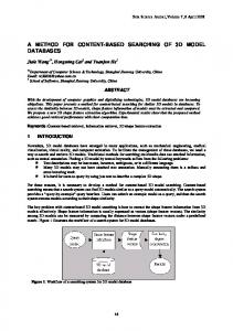
Figure 1: Fraction of the content summaries of three web-based text databases. A database selection algorithm attempts to find the best databases to evaluate a given query, based on information about the database contents. Usually this information includes the number of different documents that contain each word, to which we refer as the document frequency of the word, plus perhaps some other simple related statistics [12, 23, 35], like the number of documents NumDocs stored in the database. Figure 1 depicts a small fraction of what the content summaries for three real text databases might look like. For example, the content summary for the BioLinks database, a database with scientific articles about biology, indicates that 24 documents in this database of 13,891 documents contain the word “cancer.” Given these summaries, a database selection algorithm estimates how relevant each database is for a given query (e.g., in terms of the number of matches that each database is expected to produce for the query). To make our discussion concrete, we describe briefly below how one of these database selection algorithms works. Example 3: bGlOSS [14] is a database selection algorithm that assumes that query words are independently distributed over database documents to estimate the number of documents that match a given query. So, bGlOSS estimates that query [breast AND cancer] will match the following number of documents in database CANCERLIT: df(breast) df(cancer) · |CANCERLIT| |CANCERLIT| 121, 134 91, 688 ∼ = 148, 944 · · = 74, 544 148, 944 148, 944

#matches = |CANCERLIT| ·

where |CANCERLIT| is the number of documents in the CANCERLIT database, and df (·) is the number of documents that contain a given word. Similarly, bGlOSS estimates that a negligible number of documents will match the given query in the other two databases of Figure 1. In fact, when we evaluate the query on these three databases, CANCERLIT returns 91,688 documents, BioLinks returns 31 documents, and CNN.fn returns 9 documents. The relatively small difference between bGlOSS’s estimates and the actual number of matches at each database is expected since query words do not cooccur independently in the documents in reality, unlike what bGlOSS assumes. 2 bGlOSS is a simple example of a large family of database selection algorithms that rely on content summaries like those in Figure 1. Furthermore, database selection algorithms expect such content summaries to be accurate and up to date. The most desirable scenario is when each database exports these content summaries directly (e.g., via a protocol such as STARTS [12]). Unfortunately, no protocol is widely adopted for web-accessible text databases, and there is little hope that such a protocol will be adopted soon. For this reason, other solutions are needed to automate the

4

construction of content summaries from text databases that cannot or are not willing to export such information. We describe one such approach next.

2.2

Uniform Probing for Content Summary Construction

Callan et al. [2, 4] presented pioneer work on automatic extraction of document frequency statistics from “uncooperative” text databases that do not export such metadata. Their algorithm extracts a document sample from a given database D and computes the frequency of each observed word w in the sample, SampleDF (w): 1. Start with an empty content summary where SampleDF (w) = 0 for each word w, and a general (i.e., not specific to D), comprehensive word dictionary. 2. Pick a word (see below) and send it as a query to database D. 3. Retrieve the top-k documents returned for this query. 4. If the number of retrieved documents exceeds a prespecified threshold, stop. Otherwise continue the sampling process by returning to Step 2. Callan et al. suggested using k = 4 for Step 3 and that 300 documents are sufficient (Step 4) to create a representative content summary of the database. Also they describe two main versions of this algorithm that differ in how Step 2 is executed. The algorithm RandomSampling-OtherResource (RS-Ord for short) picks a random word from the dictionary for Step 2. In contrast, the algorithm RandomSampling-LearnedResource (RS-Lrd for short) selects the next query from among the words that have been already discovered during sampling. RS-Ord constructs better profiles, but is more expensive than RS-Lrd [4]. Other variations of this algorithm perform worse than RS-Ord and RS-Lrd, or have only marginal improvements in effectiveness at the expense of probing cost. As a result of this process, we compute the sample document frequencies SampleDF (w) for each word w that appeared in a retrieved document. These frequencies range between 1 and the number of retrieved documents in the sample. In other words, the actual document frequency ActualDF (w) for each word w in the database is not revealed by this process. This is one of the shortcomings of RS-Ord and RS-Lrd algorithms that we discuss below: Probing efficiency: One disadvantage of RS-Ord [4], is that many query probes return no documents at all. According to Zipf’s law [38], most of the words in a collection occur very few times. Hence, a word that is randomly picked from a dictionary (which hopefully contains a superset of the words in the database), is likely not to occur in any document of an arbitrary database. Hence, RS-Ord tends to produce inefficient executions in which it repeatedly issues queries to databases that produce no matches. As an example, consider the CANCERLIT database. We implemented the RS-Ord algorithm and issued 6,184 query probes to the database to extract 300 documents, which was the stopping condition in Step 4 above. Out of the 6,184 queries, only 80 (or 1.3%) matched any CANCERLIT documents. Queries that failed to return any results (e.g., “fifa”, “espresso”, “router”) are mostly associated with topics other than medicine, which is CANCERLIT ’s focus. A related problem with RS-Ord is that the information about the failure of a query to retrieve any documents is not exploited to avoid unnecessarily issuing topically similar queries. Document sample quality: By picking random queries, both RS-Ord and RS-Lrd might retrieve documents with words that might not be representative of the contents of the database. For example, the query [basketball] returns 5

14 results on CANCERLIT that discuss health problems of basketball players. These documents will be retrieved and added to the sample, increasing the sample frequency of the word “basketball” by four (this word is included in all retrieved documents). Both RS-Ord and RS-Lrd will then conclude that “basketball” is in (at least) 4 out of 300 CANCERLIT documents (or 1.33% documents), if the extracted sample consists of 300 documents. In reality, CANCERLIT has approximately 150,000 documents and [basketball] matches only 14 documents, or less than 0.01% of its documents. Hence, we can see that the “compression of scale” of the document frequencies in the [1 . . . 300] range might in principle compromise the quality of some entries in the summary. No absolute document frequencies: An additional (related) problem of both RS-Ord and RS-Lrd is that the calculated document frequencies only contain information about the relative ordering of the words in the database, without revealing information about the absolute frequencies of the words. Hence, two databases with the same focus (e.g., two medical databases) but differing significantly in size will be assigned similar content summaries. For example, CANCERLIT ’s content summary is quite similar to that of Medicine Online 6 , which contains two orders of magnitude fewer articles than CANCERLIT. Hence, a database selection algorithm that tries to maximize the number of expected matches for each query will fail to distinguish between these significantly different databases. The RS-Ord and RS-Lrd techniques extract content summaries from uncooperative text databases that otherwise could not be evaluated during a metasearcher’s database selection step. However, as discussed above, this probing technique suffers from efficiency and content summary accuracy shortcomings. In Section 3 we present a novel contentsummary construction technique that exploits earlier work on text-database classification using focused probing [18], which we review next.

2.3

Focused Probing for Database Classification

Another way to characterize the contents of a text database is to classify it in a Yahoo!-like hierarchy of topics according to the type of the documents that it contains. For example, CANCERLIT can be classified under the category “Health,” since it contains mainly health-related documents. Ipeirotis et al. [18] presented a method to automate the classification of web-accessible text databases, based on the principle of “focused probing.” The rationale behind this method is that queries closely associated with topical categories retrieve mainly documents about that category. For example, a query [breast AND cancer] is likely to retrieve mainly documents that are related to the “Health” category. By observing the number of matches generated for each such query at a database, we can then place the database in a classification scheme. For example, if one database generates a large number of matches for the queries associated with the “Health” category, and only a few matches for all other categories, we might conclude that this database should be under category “Health.” To automate this classification, these queries are derived automatically from a rule-based document classifier. A rule-based classifier is a set of logical rules defining classification decisions: the antecedents of the rules are a conjunction of words and the consequents are the category assignments for each document. For example, the following rules are part of a classifier for the two categories “Sports” and “Health”: IF jordan AND bulls THEN Sports 6 http://www.meds.com

6

Classify(Category C, Database D) Result = ∅ if (C is a leaf node) then return {C} Probe database D with the query probes derived from the classifier for the subcategories of C. Calculate Coverage and Specificity from the number of matches for the probes. foreach subcategory Ci of C if (Specificity(D, Ci ) > τs AND Coverage(D, Ci ) > τc ) then Result = Result ∪ Classify(Ci , D) if (Result == ∅) then return {C} else return Result

Figure 2: Classifying a database D into the subtree rooted at category C. IF hepatitis THEN Health IF baseball THEN Sports These rules are automatically extracted from a set of training documents that are preclassified into an existing taxonomy. For example, the first rule would classify previously unseen documents (i.e., documents not in the training set) containing the words “jordan” and “bulls” into the category “Sports.” One good property of classification rules like the ones above is that they can be easily transformed into queries. The transformation can be done by mapping each rule p → C of the classifier into a boolean query q that is the conjunction of all words in p. Thus, a query probe q sent to the search interface of a database D will match mostly documents that would fall into the category C. Categories can be further divided into subcategories, hence resulting in multiple levels of classifiers, one for each internal node of a classification hierarchy. We can then have one classifier for coarse categories like “Health” or “Sports”, and then use a different classifier that will assign the “Health” documents into subcategories like “Cancer,” “AIDS,” and so on. By applying this principle recursively for each internal node of the classification scheme, it is possible to create a hierarchical classifier that will recursively divide the space into successively smaller topics. The algorithm in [18] uses such a hierarchical scheme, and automatically maps rule-based document classifiers into queries, which are then used to probe and classify text databases. To classify a database, the algorithm in [18] starts by first sending the query probes associated with the subcategories of the top node C of the topic hierarchy, and extracting the number of matches for each probe, without retrieving any documents. Based on the number of matches for the probes for each subcategory Ci , it then calculates two metrics, the Coverage(Ci ) and Specificity(Ci ) for the subcategory. Coverage(Ci ) is the absolute number of documents in the database that are estimated to belong to Ci , while Specificity(Ci ) is the fraction of documents in the database that are estimated to belong to Ci . The algorithm decides to classify a database into a category Ci if the values of Coverage(Ci ) and Specificity(Ci ) exceed two prespecified thresholds τc and τs , respectively. These thresholds are determined by “editorial” decisions on how “coarse” a classification should be. For example, higher levels of the specificity threshold τs result in assignments of databases mostly to higher levels of the hierarchy, while lower values tend to assign the 7

databases to nodes closer to the leaves. When the algorithm detects that a database satisfies the specificity and coverage requirement for a subcategory Ci , it proceeds recursively in the subtree rooted at Ci . By not exploring other subtrees that did not satisfy the coverage and specificity conditions, we avoid exploring portions of the topic space that are not relevant to the database. This results in accurate database classification using a small number of query probes (i.e., an average of 183 probes, of between one and four words each, to classify a web-accessible database [18]). Interestingly, this database classification algorithm provides a way to zoom in on the topics that are most representative of a given database’s contents and we can then exploit it to circumvent some of the limitations of the uniform probing approach (Section 2.2) for content summary construction.

3

Focused Probing for Content Summary Construction

We now describe a novel algorithm to construct content summaries for a text database. Our algorithm exploits a topic hierarchy to adaptively send focused probes to the database. These queries tend to efficiently produce a document sample that is topically representative of the database contents, which leads to highly accurate content summaries. Furthermore, our algorithm classifies the databases along the way. In Section 4 we will exploit this categorization and the database content summaries to introduce a hierarchical database selection technique that can handle incomplete content summaries well. Our content-summary construction algorithm consists of two main steps: 1. Query the database using focused probing to (Section 3.1): (a) Retrieve a document sample. (b) Generate a preliminary content summary. (c) Categorize the database. 2. Estimate the absolute frequencies of the words retrieved from the database (Section 3.2).

3.1

Building Content Summaries from Extracted Documents

The first step of our content summary construction algorithm is to adaptively query a given text database using focused probes to retrieve a document sample. The probing process itself is closely related to that described in Section 2.3 for database classification. The new algorithm is shown in Figure 3, where we have enclosed in boxes the differences with respect to the algorithm of Figure 2. Specifically, for each query probe we now retrieve k documents from the database in addition to the number of matches that the probe generates (box β in Figure 3). Also, we record two sets of word frequencies based on the probe results and extracted documents (boxes β and γ): 1. ActualDF (w): the actual number of documents in the database that contain word w. The algorithm knows this number only if [w] is a single-word query probe that was issued to the database7 . 2. SampleDF (w): the number of documents in the extracted sample that contain word w. 7 The

number of matches reported by a database for a single-word query [w] might differ slightly from ActualDF (w), for example, if the

database applies stemming [30] to query words so that a query [computers] also matches documents with word “computer.”

8

GetContentSummary(Category C, Database D) α: hSampleDF , ActualDF i = h∅, ∅i if (C is a leaf node) then return hSampleDF , ActualDF i Probe database D with the query probes derived from the classifier for the subcategories of C newdocs = ∅ foreach query probe q newdocs = newdocs ∪ {top-k documents returned for q} β:

if q consists of a single word w then ActualDF (w) = #matches returned for q foreach word w in newdocs SampleDF (w) = #documents in newdocs that contain w

Calculate Coverage and Specificity from the number of matches for the probes foreach subcategory Ci of C if (Specificity(D, Ci ) > τs AND Coverage(D, Ci ) > τc ) then γ:

hSampleDF ’, ActualDF ’i = GetContentSummary(Ci , D) Merge hSampleDF ’, ActualDF ’i into hSampleDF , ActualDF i

return hSampleDF , ActualDF i

Figure 3: Generating a content summary for a database D using focused query probing. The basic structure of the probing algorithm follows that of the one described in Section 2.3 (Figure 2). In a nutshell, we explore (and send query probes for) only those categories with sufficient specificity and coverage, as determined by the τs and τc thresholds. As a result, this algorithm categorizes the databases into the classification scheme during the probing process. We will exploit this categorization in our database selection algorithm of Section 4. Figure 4 illustrates how our algorithm works for the CNN Sports Illustrated database8 , a database with articles about sports, and for a hierarchical scheme with four categories under the root node: “Sports,” “Health,” “Computers,” and “Science.” We pick specificity and coverage thresholds τs = 0.5 and τc = 100, respectively. The algorithm starts by issuing the query probes associated with each of the four categories. As we can see from the figure, the “Sports” probes generate many matches (e.g., query [baseball] matches 24,520 documents). In contrast, the probes for the other sibling categories (e.g., [metallurgy] for category “Science”) generate just a few or no matches. The Coverage of category “Sports” is the sum of the number of matches for its probes, or 32,050. The Specificity of category “Sports” is the fraction of matches that correspond to “Sports” probes, or 0.967. Hence, “Sports” satisfies the Specificity and Coverage criteria (recall that τs = 0.5 and τc = 100) and is further explored to the next level of the hierarchy. In contrast, “Health,” “Computers,” and “Science” are not considered further. The benefit of this pruning of the probe space is two-fold: First, we improve the efficiency of the probing process by giving attention to the topical focus (or foci) of the database. (Out-of-focus probes would tend to return few or no matches.) Second, we avoid retrieving spurious matches and focus on documents that are better representatives of the database being summarized. 8 http://www.cnnsi.com

9

Figure 4: Querying the CNN Sports Illustrated database with focused probes. During probing, our algorithm retrieves the top-k documents returned by each query (box β in Figure 3). For each word w in a retrieved document, the algorithm computes SampleDF (w) by measuring the number of documents in the sample, extracted in a probing round, that contain w. If a word w appears in document samples retrieved during later phases of the algorithm for deeper levels of the hierarchy, then all SampleDF (w) values are added together (“merge” step in box γ). Similarly, during probing the algorithm keeps track of the number of matches produced by each singleword query [w]. As discussed, the number of matches for such a query is (a close approximation to) the ActualDF (w) frequency (i.e., the number of documents in the database with word w). These ActualDF (·) frequencies will be crucial to estimate the absolute document frequencies of all words that appear in the document sample extracted, as we discuss next.

3.2

Estimating Absolute Documents Frequencies

No probing technique so far has been able to estimate the absolute document frequency of words. As discussed, the RS-Ord and RS-Lrd techniques of Callan et al. [4] will “squeeze” all estimated document frequencies in the [1 . . . N ] range, where N is the number of documents extracted during probing (e.g., 300). Hence, database selection algorithms could not distinguish between two databases with similar topic coverage but with orders of magnitude difference in sizes. We now show how we can exploit the ActualDF (·) and SampleDF (·) document frequencies that we extract from a database (Section 3.1) to build a content summary for the database with accurate absolute document frequencies. For this, we follow two basic steps: 1. Exploit the SampleDF (·) frequencies derived from the document sample to rank all observed words from most

10

Figure 5: Estimating unknown ActualDF values. frequent to least frequent. 2. Exploit the ActualDF (·) frequencies derived from one-word query probes to potentially boost the document frequencies of “nearby” words w for which we only know SampleDF (w) but not ActualDF (w). Figure 5 illustrates our technique for CANCERLIT. After probing CANCERLIT using the algorithm in Figure 3, we rank all words in the extracted documents according to their SampleDF (·) frequency. In this figure, “cancer” has the highest SampleDF value and “hepatitis” the lowest such value. The SampleDF value of each word is noted by the corresponding vertical bar. Also, the figure shows the ActualDF (·) frequency of those words that formed single-word queries. For example ActualDF (hepatitis) = 20, 000, because query probe [hepatitis] returned 20,000 matches. Note that the ActualDF value of some words (e.g., “stomach”) is unknown. These words appeared in documents that we retrieved during probing, but not as single-word probes. From the figure, we can see that SampleDF(hepatitis) ≈ SampleDF(stomach). Then, intuitively, we will estimate ActualDF (stomach) to be close to the (known) value of ActualDF (hepatitis). To specify how to “propagate” the known ActualDF frequencies to “nearby” words with similar SampleDF frequencies, we exploit well-known laws on the distribution of words over text documents. Zipf [38] was the first to observe that word-frequency distributions follow a power law, which was later refined by Mandelbrot [22]. Mandelbrot observed a relationship between the rank r and the frequency f of a word in a text database: f = P (r + p)−B

(1)

where P , B, and p are parameters of the specific document collection. This formula indicates that the most frequent word in a collection (i.e., the word with rank r = 1) will tend to appear in P (1 + p)−B documents, while, say, the tenth most frequent word will appear in just P (10 + p)−B documents. Just as in Figure 5, after probing we know the rank of all observed words in the sample documents retrieved, as well as the actual frequencies of some of those words in the entire database. These statistics, together with Equation 1 11

above, lead to the following procedure for estimating unknown ActualDF (·) frequencies: 1. Sort all words in descending order of their SampleDF (·) frequencies to determine the rank ri of each word wi . 2. Focus on words with known ActualDF (·) frequencies. Use the SampleDF -based rank and ActualDF frequencies to find the P , B, and p parameter values that best fit the data (Equation 1 above). 3. Estimate ActualDF (wi ) for all words wi with unknown ActualDF (wi ) as P (ri + p)−B , where ri is the rank of word wi as computed in Step 1. For Step 2, we use an off-the-shelf curve fitting algorithm available as part of the R-Project 9 , an open-source environment for statistical computing. Example 4: Consider database CANCERLIT and Figure 5.

We know that ActualDF(hepatitis) = 20, 000 and

ActualDF(liver) = 140, 000, since the respective one-word query probes reported so many matches in each case. Additionally, using the SampleDF frequencies, we know that “liver” is the fifth most popular word among the extracted documents, while “hepatitis” ranked number 25. Similarly, “kidneys” is the 10th most popular word. Unfortunately, we do not know the value of ActualDF(kidneys) since [kidneys] was not a query probe. However, using the ActualDF frequency information from the other words and their SampleDF-based rank, we estimate the distribution parameters in Equation 1 to be P = 8.105 , p = 0.25, and B = 1.15. Using the rank information with Equation 1, we compute ActualDFest (kidneys) = 8.105 (10 + 0.25)−1.15 ∼ = 55, 000. In reality, ActualDF(kidneys) = 65, 000, which is close to our estimate. 2 During sampling, we also send to the database query probes that consist of more than one word. (Recall that our query probes are derived from an underlying, automatically learned document classifier.) We do not exploit multi-word queries for determining ActualDF frequencies of their words, since the number of matches returned by a boolean-AND multi-word query is only a lower bound on the ActualDF frequency of each intervening word. However, the average length of the query probes that we generate is small (less than 1.5 in our experiments), and their median length is one. Hence, the majority of the query probes provides us with ActualDF frequencies that we can exploit. Another interesting observation is that we can derive a gross estimate of the number of documents in a database as the largest (perhaps estimated) ActualDF frequency, since the most frequent words tend to appear in a large fraction of the documents in a database. In summary, we presented a focused probing technique for content summary construction that (a) estimates the absolute document frequency of the words in a database, and (b) automatically classifies the database in a hierarchical classification scheme along the way. We show next how we can define a database selection algorithm that uses the content summary and categorization information of each available database.

4

Exploiting Topic Hierarchies for Database Selection

Any efficient algorithm for constructing content summaries through query probes is likely to produce incomplete content summaries, which can affect the effectiveness of the database selection process. Specifically, database selection would 9 http://www.r-project.org/

12

Figure 6: Associating content summaries with categories. suffer the most for queries with one or more words not present in content summaries. We now introduce a database selection algorithm that exploits the database categorization and content summaries produced as in Section 3 to alleviate the negative effect of incomplete content summaries. This algorithm consists of two basic steps: 1. “Propagate” the database content summaries to the categories of the hierarchical classification scheme (Section 4.1). 2. Use the content summaries of categories and databases to perform database selection hierarchically by zooming in on the most relevant portions of the topic hierarchy (Section 4.2).

4.1

Creating Content Summaries for Topic Categories

Sections 2.3 and 3 showed algorithms for extracting database content summaries. These summaries could be used to guide existing database selection algorithms such as CORI [3] or bGlOSS [14]. However, these algorithms might produce inaccurate conclusions for queries with one or more words missing from relevant content summaries. This is particularly problematic for the short one- or two-word queries that are prevalent over the web. A first step to alleviate this problem is to associate content summaries to the categories of the topic hierarchy used by the probing algorithm of Section 3. In the next section, we use these category content summaries to select databases hierarchically. The intuition behind our approach is that databases classified under similar topics tend to have similar vocabularies. Hence, we can view the (potentially incomplete) content summaries of all databases in a category as complementary, and exploit this view for better database selection. For example, consider the CANCERLIT database and its associated content summary in Figure 6. As we can see, CANCERLIT was correctly classified under “Cancer” by the algorithm in Section 3. Unfortunately, the word “metastasis” did not appear in any of the documents extracted from CANCERLIT

13

during probing, so this word is missing from the content summary. However, we see that CancerBACUP 10 , another database classified under “Cancer”, has a high ActualDFest (metastasis) = 3, 569. Hence, we might conclude that the word “metastasis” did not appear in CANCERLIT because it was not discovered during sampling, and not because it does not occur in the CANCERLIT database. We convey this information by associating a content summary to category “Cancer” that is obtained by merging the summaries of all databases under this category. In the merged content summary, ActualDFest (w) is the sum of the document frequency of w for databases under this category. In general, the content summary of a category C with databases db1 , . . . , dbn classified (not necessary immediately) under C includes: • NumDBs(C): The number of databases under C (n in this case). • NumDocs(C): The number of documents in any dbi under C; NumDocs(C)=

P dbi

NumDocs(dbi ).

• ActualDFest (w): The number of documents in any dbi under C that contain the word w; ActualDFest (w) = P dbi (ActualDFest (w)for dbi ). By having content summaries associated with categories, we can treat each category as a large “database” and perform database selection hierarchically; we describe one possible algorithm for this task next.

4.2

Selecting Databases Hierarchically

Now that we have associated content summaries with the categories in the topic hierarchy, we can select databases for a query hierarchically, starting from the top category. At each level, we use existing flat database algorithms such as CORI [3] or bGlOSS [14]. These algorithms assign a score to each database (or category in our case) for a query, which specifies how promising the database (or category) is for the query, based on its content summary (see Example 3). We assume in our discussion that scores are greater than or equal to zero, with a zero score indicating that a database or category should be ignored for the query. Given the scores for the categories at one level of the hierarchy, the selection process will continue recursively onto the most promising subcategories. There are several alternative strategies that we could follow to decide what subcategories to exploit. In this paper, we present one such strategy, which privileges topic-specific over broader databases. Earlier research indicated that distributed information retrieval systems tend to produce better results when documents are organized in topically-cohesive clusters [36, 20]. Figure 7 summarizes our hierarchical database selection algorithm. The algorithm takes as input a query Q and the target number of databases K that we are willing to search for the query. Also, the algorithm receives the top category C as input, and starts by invoking a flat database selection algorithm to score all subcategories of C for the query (Step 1), using the content summaries associated with the subcategories (Section 4.1). If at least one “promising” subcategory has a non-zero score (Step 2), then the algorithm picks the best such subcategory Cj (Step 3). If Cj has K or more databases under it (Step 4) the algorithm proceeds recursively under that branch only (Step 5). As discussed above, this strategy privileges “topic-specific” databases over databases with broader scope. On the other hand, if Cj does not have sufficiently many (i.e., K or more) databases (Step 6), then intuitively the algorithm has gone as deep in 10 http://www.cancerbacup.org.uk

14

HierSelect(Query Q, Category C, int K) 1: Use a database selection algorithm to assign a score for Q to each subcategory of C. 2: if there is a subcategory C with a non-zero score 3:

Pick the subcategory Cj with the highest score

4:

if NumDBs(Cj ) ≥ K /* Cj has enough databases */

5: 6: 7:

return HierSelect(Q,Cj ,K) else /* Cj does not have enough databases */ return DBs(Cj ) ∪ FlatSelect(Q,C − Cj ,K-NumDBs(Cj ))

8: else /* no subcategory C has non-zero score */ 9:

return FlatSelect(Q,C,K)

Figure 7: Selecting the K most specific databases for a query hierarchically.

Figure 8: Exploiting a topic hierarchy for database selection. the hierarchy as possible (exploring only category Cj would result in fewer than K databases being returned). Then, the algorithm returns all NumDBs(Cj ) databases under Cj , plus the best K − NumDBs(Cj ) databases under C but not in Cj , according to the “flat” database selection algorithm of choice (Step 7). If no subcategory of C has a non-zero score (Step 8), again this indicates that the execution has gone as deep in the hierarchy as possible. Therefore, we return the best K databases under C, according to the flat database selection algorithm (Step 9). Figure 8 shows an example of an execution of this algorithm for query [babe AND ruth]. We start with a target of K = 3 databases. The top-level categories are evaluated by a flat database selection algorithm for the query, and the “Sports” category is deemed best, with a score of 0.93. Since the “Sports” category has more than three databases, the query is “pushed” into this category. The algorithm proceeds recursively by pushing the query into the “Baseball” category. If we had initially picked K = 10 instead, the algorithm would have still picked “Sports” as the first category to explore. However, “Baseball” has only 7 databases, so the algorithm picks them all, and chooses the best 3 databases under “Sports” to reach the target of 10 databases for the query. In summary, our hierarchical database selection algorithm chooses the best, most-specific databases for a query. By exploiting the database categorization, this hierarchical algorithm manages to compensate for the necessarily incomplete database content summaries produced by query probing. In the next sections we evaluate the performance of this algorithm against that of “flat” database selection techniques. 15

Web Database

URL

UM Comprehensive Cancer Center

http://www.cancer.med.umich.edu/search.htm

Java @ Sun.com

http://search.java.sun.com

Johns Hopkins AIDS Service

http://hopkins-aids.edu/index search.html

SportSearch

http://sportsearch.com/search.cgi

Duke Papyrus Archive

http://scriptorium.lib.duke.edu/papyrus/

Table 1: Some of the real web databases in the Web set.

5

Data and Metrics

In this section we describe the data (Section 5.1) and techniques (Section 5.2) that we use for the experiments reported in Section 6.

5.1

Experimental Setting

To evaluate the algorithms described in this paper, we use two data sets: one set of “Controlled” databases that we assembled locally with newsgroup articles, and another set of “Web” databases, which we could only access through their web search interface. We also use a 3-level subset of the Yahoo! topic hierarchy consisting of 72 categories, with 54 “leaf” topics and 18 “internal” topics. Controlled Database Set: We gathered 500,000 newsgroup articles from 54 newsgroups during April-May 2000. Out of these, we used 81,000 articles to train document classifiers over the 72-node topic hierarchy. For training we manually assigned newsgroups to categories, and treated all documents from a newsgroup as belonging to the corresponding category. We used the remaining 419,000 articles to build the set of Controlled Databases. This set contained 500 databases ranging in size from 25 to 25,000 documents. 350 of them were “homogeneous,” with documents from a single category, while the remaining 150 are “heterogeneous,” with a variety of category mixes. We define a database as “homogeneous” when it has articles from only one node, regardless of whether this node is a leaf or not. If a database corresponds to an internal node, then it has equal number of articles from each leaf node in its subtree. The “heterogeneous” databases, on the other hand, have documents from different categories that reside in the same level in the hierarchy (not necessarily siblings), with different mixture percentages. These databases were indexed and queried by a SMART-based program [31] using the cosine similarity function with tf.idf weighting [29]. Web Database Set: We used a set of 50 real web-accessible databases over which we do not have any control. These databases were picked randomly from two directories of hidden-web databases, namely InvisibleWeb11 and CompletePlanet12 . These databases have articles that range from research papers to film reviews. Table 1 shows a sample of five databases from the Web set. For each database in the Web set, we constructed a simple wrapper to send a query and retrieve the number of matches and the documents returned in the first page of query results. 11 http://www.invisibleweb.com/ 12 http://www.completeplanet.com/

16

5.2

Alternative Techniques

Our experiments evaluate two main sets of techniques: content-summary construction techniques (Sections 2 and 3) and database selection techniques (Section 4): Content Summary Construction: We test variations of our Focused Probing technique against the two main variations of uniform probing, described in Section 2.2, namely RS-Ord and RS-Lrd. As the initial dictionary D for these two methods we used the set of all the words that appear in the databases of the Controlled set. For Focused Probing, we evaluate configurations with different underlying document classifiers for query-probe creation, and different values for the thresholds τs and τc that define the granularity of sampling performed by the algorithm in Figure 3. Specifically, we consider the following variations of the Focused Probing technique: • FP-RIPPER: Focused Probing using RIPPER [5] as the base document classifier (Section 3.1). • FP-C4.5: Focused Probing using C4.5RULES [28], which extracts classification rules from decision tree classifiers generated by C4.5 [28]. • FP-Bayes: Focused Probing using Naive-Bayes classifiers [9] in conjunction with a rule-extraction technique to extract rules from numerically-based Naive-Bayes classifiers [39]. • FP-SVM: Focused Probing using Support Vector Machines with linear kernels [19] in conjunction with the same rule-extraction technique used for FP-Bayes. We vary the specificity threshold τs to get document samples of different granularity. All variations were tested with threshold τs ranging between 0 and 1. Low values of τs result in databases being “pushed” to more categories, which in turn results in larger document samples. To keep the number of experiments manageable, we fix the coverage threshold to τc = 10, varying only the specificity threshold τs . Database Selection Effectiveness: We test variations of our database selection algorithm of Section 4 along several dimensions: • Underlying Database Selection Algorithm: The hierarchical algorithm of Section 4.2 relies on a “flat” database selection algorithm. We consider two such algorithms: CORI [3] and bGlOSS [14]. Our purpose is not to evaluate the relative merits of these two algorithms (for this, see [10, 27]) but rather to ensure that our techniques behave similarly for different flat database selection algorithms. We adapted both algorithms to work with the category content summaries described in Section 4.1. • Content Summary Construction Algorithm: We evaluated how our hierarchical database selection algorithm behaves over content summaries generated by different techniques. In addition to the content-summary construction techniques listed above, we also test QPilot, a recent strategy that exploits HTML links to characterize text databases [33]. Specifically, QPilot builds a content summary for a web-accessible database D as follows: 1. Query a general search engine to retrieve pages that link to the web page for D13 . 13 QPilot

finds backlinks by querying AltaVista using queries of the form “link:URL-of-the-database.” [33]

17

(a)

(b)

Figure 9: The ctf ratio (a) and the Spearman Rank Correlation Coefficient (b) for different methods and for different values of the specificity threshold τs . 2. Retrieve the top-m pages that point to D (e.g., m = 50). 3. Extract the words in the same line as a link to D. 4. Include only words with high document frequency in the content summary for D. • Full Documents vs. Snippets: So far we have assumed that we retrieve full documents during probing to build content summaries. An interesting alternative is to exploit the anchor text and snippets that often accompany each link to a document in a query result. These snippets are short summaries of the documents that are often query-specific. Using snippets, rather than full documents, yields more efficient content summary construction, at the expense of less complete content summaries. • Hierarchical vs. Flat Database Selection: We compare the effectiveness of the hierarchical algorithm of Section 4.2, against that of the underlying “flat” database selection strategies.

6

Experimental Results

We use the Controlled database set for experiments on content summary quality (Section 6.1), while we use the Web database set for experiments on database selection effectiveness (Section 6.2). We report the results next.

6.1

Content Summary Quality

Coverage of the retrieved vocabulary: An important property of content summaries is their coverage of the actual database vocabulary. To measure coverage, we use the ctf ratio metric introduced in [4]: P ActualDF (w) ctf = Pw∈Ts w∈Td ActualDF (w) 18

(2)

where Ts is the set of terms in a content summary and Td is the complete set of words in the corresponding database. This metric gives higher weight to more frequent words, but is calculated after stopwords (e.g., “a”, “the”) are removed, so this ratio is not artificially inflated by the discovery of very common words. We report the ctf ratio for the different content summary construction algorithms in Figure 9(a). The variants of the Focused Probing technique achieve much higher ctf ratios than RS-Ord and RS-Lrd do. Early during probing, Focused Probing retrieves documents covering different topics, and then sends queries of increasing specificity, retrieving documents with more specialized words. As expected, the coverage of the Focused Probing summaries increases for lower thresholds of τs , since the number of documents retrieved for lower thresholds is larger: a sample of larger size, everything else being the same, is better for content summary construction. The difference between RS-Lrd and RS-Ord is small. RS-Lrd has slightly lower ctf values, due to the bias induced from querying only using previously discovered words. Correlation of word rankings: The ctf ratio can be helpful to compare the quality of different content summaries. However, this metric alone is not enough, since it does not capture the relative “rank” of words in the content summary by their observed frequency. To measure how well a content summary orders words by frequencies with respect to the actual word frequency order in the database, we use the Spearman Rank Correlation Coefficient (SRCC for short): P P 3 P 1 1 (g 3 − gm )) 1 − n36−n ( i d2i + 12 k (fk − fk ) + 12 P 3 P 3 m m (3) SRCC = p (fk −fk ) p (g −gm ) (1 − kn3 −n ) (1 − mn3 m ) −n where di is the rank difference of the word i, n is the number of words, fk is the number of ties in the kth group in the ranking calculated using SampleDF and gm is the number of ties in the mth group in the ranking calculated using ActualDF. When two rankings are identical then SRCC =1; when they are uncorrelated, SRCC =0; and when they are in reverse order, SRCC =-1. The results for the different algorithms are listed in Figure 9(b). Again, the content summaries produced by the Focused Probing techniques have much higher SRCC values than for RS-Lrd and RS-Ord, hinting that Focused Probing retrieves a more representative sample of documents. Accuracy of frequency estimations: In Section 3.2 we introduced a technique to estimate the actual absolute frequencies of the words in a database. To evaluate the accuracy of our predictions, we report the average relative error for words with actual frequencies greater than three. (Including the large tail of less-frequent words would highly distort the relative-error computation.) Figure 10(a) reports the average relative error estimates for our algorithms. We also applied our absolute frequencies estimation algorithm of Section 3.2 to RS-Ord and RS-Lrd, even though this estimation is not part of the original algorithms in [4]. As a general conclusion, our technique provides a good ballpark estimate of the absolute frequency of the words. Efficiency: To measure the efficiency of the probing methods, we report the sum of the number of queries sent to a database and the number of documents retrieved (“number of interactions”) in Figure 10(b). Except for the case of RS-Ord, which unnecessarily issues many queries that produce no document matches (Section 2.2), the efficiency of the other techniques is correlated with their effectiveness. The more expensive techniques tend to give better results. The exception is FP-SVM, which has the lowest cost among all the methods for τs > 0 and still gives results of comparable quality with respect to the more expensive methods. We also measured how often the probes sent by the different

19

(a) The average relative error for the ActualDF esti-

(b) The average number of interactions per database.

mations for words with ActualDF > 3. Figure 10: Comparison of different methods for different values of the specificity threshold τs . techniques manage to retrieve new documents from the database. We have seen that, on average, the probes for RSOrd retrieve one document every 20 probes, the probes for RS-Lrd retrieve one document every two probes, while the Focused Probing techniques retrieve one document per probe. The probes generated from the Focused Probing techniques were generally short, with a maximum of four words and a median of one word per query. Overall, the Focused Probing techniques produce significantly better-quality summaries than RS-Ord and RS-Lrd do, both in terms of vocabulary coverage and word-ranking preservation. The cost of Focused Probing in terms of number of interactions with the databases is comparable to or less than that for RS-Lrd, and significantly less than that for RS-Ord. Finally, the absolute frequency estimation technique of Section 3.2 gives good ballpark approximations of the actual real-world frequencies.

6.2

Database Selection Effectiveness

The Controlled set allowed us to carefully evaluate the quality of the content summaries that we extract. We now turn to the Web set of real web-accessible databases to evaluate how the quality of the content summaries affects the database selection task. Additionally, we evaluate how the hierarchical database selection algorithm of Section 4.2 improves the selection task. Evaluation metrics: We used the queries 451-500 from the Web Track of TREC-9 [16]. TREC is a conference for the large-scale evaluation of text retrieval methodologies. In particular, the Web Track evaluates methods for retrieval of web content. TREC provides both web pages and queries as part of its Web Track. We use the queries for our database selection experiments over the Web database set described in Section 5.1. (We ignored the “flat” set of TREC web pages since we are interested in evaluating algorithms for choosing databases, not individual pages or documents.) Table 2 shows two queries from the Web Track of TREC-9. Our evaluation proceeded as follows for each of the 50 TREC queries. Each database selection algorithm (Section 5.2) picked three databases for the query. We then retrieved the top-5 documents for the query from each selected database.

20

#Topic

Query

Description

Relevance-Evaluation Guidelines

453

[hunger]

Find documents that discuss orga-

Relevant documents contain the name of any organization or

nizations/groups that are aiding in

group that is attempting to relieve the hunger problem in the

the eradication of the worldwide

world. Documents that address the problem only without

hunger problem.

providing names of organizations/groups that are working on hunger are irrelevant.

482

[where can i find

Find documents that give growth

Document that give heights of trees but not the rate of

growth rates for

rates of pine trees.

growth are not relevant.

the pine tree]

Table 2: Two different queries from topics 451-500 of TREC. Content Summary Generation Technique

CORI

bGlOSS

Hierarchical

Flat

Hierarchical

Flat

FP-SVM-Docs

0.27

0.178

0.163

0.085

FP-SVM-Snippets

0.2

0.183

0.093

0.090

RS-Ord

-

0.177

-

0.085

QPilot

-

0.052

-

0.008

Table 3: The average precision of different database selection algorithms for topics 451-500 of TREC. This procedure resulted in (at most) 15 documents for the query for each algorithm. The relevance [30] of these 15 documents is what ultimately reveals the quality of each algorithm. We asked human evaluators to judge the relevance of each retrieved document for the query following the guidelines given by TREC for each query (Table 2). Then, the precision of a technique for each query q is: Pq =

|relevant documents in the answer| |total number of documents in the answer|

(4)

We report the average precision achieved by each database selection algorithm over the 50 TREC WebTrack queries. Human relevance judgments are the ultimate evaluation metric of information retrieval systems [30]. Unfortunately, these judgments are highly expensive to produce. To be able to study the database selection algorithms under a larger variety of scenarios, we also conduct experiments for a metric that is less expensive to compute. Specifically, we use the number of matches produced by a database for a query as an indication of how relevant the database is for the query. Then, given a set of k databases DB chosen for a query q by a database selection algorithm, we define: P D∈DB #matches for q in D Rq = total #matches for query q over all databases

(5)

In other words, Rq measures the fraction of overall available document matches for q that is captured by querying the k databases chosen by a database selection algorithm for the query. The average precision results are reported in Table 3. We do not include in these averages the 15 queries for which all database selection algorithms either selected only databases that return zero documents or failed to select any database giving to all databases a zero score. The average R-metric results are reported in Figure 11. We discuss these figures below. Our database selection algorithm of Section 4.2 chooses databases hierarchically. We evaluate the performance of the algorithm using content summaries extracted from FP-SVM probing (Section 5.2) with specificity threshold τs = 0.25: 21

FP-SVM exhibits the best accuracy-efficiency tradeoff (Section 6.1) while τs = 0.25 leads to good database classification decisions for web databases [18]. We compare two versions of the algorithm, one using CORI [3] as the underlying flat database selection strategy, and another using bGlOSS [14]. Note that QPilot, RS-Ord, and RS-Lrd do not classify databases while building content summaries, hence we did not evaluate our hierarchical database selection algorithm over their content summaries. Table 3 shows the average precision of the hierarchical algorithms against that of flat database selection algorithms over the same content summaries, while Figure 11 shows the average R-metric values. A clear conclusion is that proceeding hierarchically helps: Hierarchical vs. flat database selection: For both types of evaluation the hierarchical versions of the database selection algorithms gave better results than their flat counterparts. For example, the hierarchical algorithm using CORI as flat database selection has 50% better precision than CORI for flat selection with the same content summaries. For bGlOSS, the improvement in precision is even more dramatic at 92%. The R metric values also show that the hierarchical algorithms exhibit superior performance compared to the other algorithms. Our hypothesis for this improvement of hierarchical selection algorithms over their flat counterparts is that the topic hierarchy helps compensate for incomplete content summaries. For example, in Figure 6 a query on [metastasis] would not be routed to the CANCERLIT database by a database selection algorithm like bGlOSS because “metastasis” is not in the CANCERLIT content summary. In contrast, our hierarchical algorithm exploits the fact that “metastasis” appears in the summary for CancerBACUP, which is in the same category as CANCERLIT, to allow CANCERLIT to be selected when the “Cancer” category is selected (the ActualDFest (metastasis) frequency from CancerBACUP propagates to the content summary of the “Cancer” category). To quantify how frequent this phenomenon is, we measured the fraction of times that our hierarchical database selection algorithm picked a database for a query that both: (a) indeed produced matches for the query, and (b) was given a zero score by the flat database selection algorithm of choice. Interestingly, this was the case for 34% of the databases picked by the hierarchical algorithm with bGlOSS and for 23% of the databases picked by the hierarchical algorithm with CORI. These numbers support our hypothesis that hierarchical database selection compensates for content-summary incompleteness. Effect of different content summaries: To analyze the effect of content summary construction algorithms on database selection, we tested how the quality of content summaries generated by RS-Ord, Focused Probing, and QPilot affect the database selection process. We picked RS-Ord over RS-Lrd because of its superior performance in the evaluation of Section 6.1. Furthermore, we applied our technique of Section 3.2 for ActualDF estimation to the RS-Ord summaries. In Table 3 we can see that, surprisingly, the gap in performance between the flat selection algorithms that use FP-SVM and RS-Ord summaries was narrower than the gap in quality of the corresponding content summaries (Section 6.1). (The phenomenon is also apparent for the R-metric values in Figure 11.) All the flat selection techniques suffer from the incomplete coverage of the underlying probing-generated summaries. A clear conclusion is that QPilot summaries do not work well for database selection because they generally contain only a few words and are hence highly incomplete. Full documents vs. snippets: Finally, we measured the impact of using just the snippets rather than full documents during content summary construction. We tested database selection over FP-SVM content summaries generated from full documents (FP-SVM-Docs), and from just snippets (FP-SVM-Snippets). Interestingly, the performance of flat database selection algorithms for FP-SVM-Docs and FP-SVM-Snippets was very similar. An explanation for this 22

(a)

(b)

Figure 11: The R metric for different algorithms using (a) bGlOSS or (b) CORI as the underlying flat database selection algorithm of choice, as a function of the number of databases selected. is that snippets tend to contain highly-descriptive document portions (e.g., title and sentences that are relevant to the query). Hence, by retrieving only these parts it might be possible to create content summaries that are at least as good as their flat counterparts. In contrast, the performance of hierarchical database selection algorithms did suffer when we use the (less complete) summaries that result from only inspecting snippets.

7

Related Work

A large body of work has been devoted to the task of database selection. Many database selection algorithms [14, 23, 35, 37, 3] rely on content summaries of the databases for this task. Some algorithms rely on hierarchical schemes [8, 7, 32, 13] to direct the queries to the appropriate nodes of the hierarchy. Some of these approaches rely either on access to all documents or on metadata directly exported by the databases. Unfortunately, web-accessible databases rarely export such metadata. Recently, Etzioni and Sugiura [33] proposed the QPilot technique, which uses query expansion to route web queries to the appropriate search engines (Section 5.2). Callan et al. [4, 2] suggested using query probes to extract document samples from databases for content summary construction (Section 2.2). Craswell et al. [6] compared the performance of different flat database selection algorithms in the presence of such content summaries. For database classification, Gauch et al. [11] manually construct query probes to facilitate the classification of text databases. Ipeirotis et al. [18] used focused query probing to automatically classify a database in a hierarchical classification scheme. In this paper we have built on the results in [18] to create an effective algorithm for content summary extraction that classifies databases while extracting document samples. This classification is used in the hierarchical database selection algorithm that we proposed in Section 4. Earlier results indicated that clustering of documents by topic may help in the database selection process [36, 20, 34]. Hawking and Thistlewaite [17] used query probing at query time to perform database selection by ranking databases by similarity to a given query. Their algorithm assumed that query interfaces can handle normal queries and query

23

probes differently and that the cost to handle query probes is smaller than that for normal queries. Meng et al. [24] used query probing to determine sources of heterogeneity in the algorithms used to index and search locally at each text database. Etzioni et al. [26] used query probes to automatically understand web-accessible query forms to build a comparative shopping agent. In [15] query probing was employed to determine the frequency of usage of different languages on the web. Outside of the field of text databases, biased sampling has been suggested as an alternative to uniform sampling. Biased sampling has been shown to perform better when the numeric data follows Zipfian distributions [25]. Biased sampling has also been used to produce more representative samples of numeric data for aggregate queries [1].

8

Conclusions

In this paper we presented a novel and efficient method for the construction of content summaries of web-accessible text databases. Our algorithm creates content summaries of higher quality than current approaches and, additionally, categorizes databases in a classification scheme. We also presented a hierarchical database selection algorithm that exploits the database content summaries and the generated classification to produce accurate results even for imperfect content summaries. Experimental results show the superiority of our techniques over the state of the art in contentsummary construction and database selection.

References [1] Swarup Acharya, Phillip B. Gibbons, and Viswanath Poosala. Congressional samples for approximate answering of group-by queries. In Proceedings of the 2000 ACM SIGMOD International Conference on Management of Data (SIGMOD 2000), pages 487–498, 2000. [2] James P. Callan, Margaret Connell, and Aiqun Du. Automatic discovery of language models for text databases. In Proceedings of the 1999 ACM SIGMOD International Conference on Management of Data (SIGMOD’99), pages 479–490, 1999. [3] James P. Callan, Zhihong Lu, and W.Bruce Croft. Searching distributed collections with inference networks. In Proceedings of the 18th Annual International ACM SIGIR Conference on Research and Development in Information Retrieval, SIGIR’95, pages 21–28, 1995. [4] Jamie Callan and Margaret Connell. Query-based sampling of text databases. ACM Transactions on Information Systems, 19(2):97–130, 2001. [5] William W. Cohen. Learning trees and rules with set-valued features. In Proceedings of the 13th National Conference on Artificial Intelligence (AAAI-96) Eighth Conference on Innovative Applications of Artificial Intelligence (IAAI-96), pages 709–716, 1996. [6] Nick Craswell, Peter Bailey, and David Hawking. Server selection on the World Wide Web. In Proceedings of the Fifth ACM Conference on Digital Libraries (DL 2000), pages 37–46, 2000. [7] R. Dolin, D. Agrawal, A. El Abbadi, and J. Pearlman. Using automated classification for summarization and selection of usenet newsgroups. D-Lib Magazine, January 1998. [8] Ron Dolin, Divyakant Agrawal, and Amr El Abbadi. Scalable collection summarization and selection. In Proceedings of the Fourth ACM International Conference on Digital Libraries (DL’99), pages 49–58, 1999. [9] Richard O. Duda and Peter E. Hart. Pattern Classification and Scene Analysis. Wiley, 1973. [10] James C. French, Allison L. Powell, James P. Callan, Charles L. Viles, Travis Emmitt, Kevin J. Prey, and Yun Mou. Comparing the performance of database selection algorithms. In Proceedings of the 22nd Annual International ACM SIGIR Conference on Research and Development in Information Retrieval, SIGIR’99, pages 238–245, 1999. [11] Susan Gauch, Guijun Wang, and Mario Gomez. ProFusion*: Intelligent fusion from multiple, distributed search engines. The Journal of Universal Computer Science, 2(9):637–649, September 1996. [12] Luis Gravano, Chen-Chuan K. Chang, H´ector Garc´ıa-Molina, and Andreas Paepcke. STARTS: Stanford proposal for Internet meta-searching. In Proceedings of the 1997 ACM SIGMOD International Conference on Management of Data (SIGMOD’97), pages 207–218, 1997.

24

[13] Luis Gravano and H´ector Garc´ıa-Molina. Generalizing GlOSS to vector-space databases and broker hierarchies. In Proceedings of the 21st International Conference on Very Large Databases (VLDB’95), pages 78–89, 1995. [14] Luis Gravano, H´ector Garc´ıa-Molina, and Anthony Tomasic. GlOSS: Text-source discovery over the Internet. ACM Transactions on Database Systems, 24(2):229–264, June 1999. [15] Gregory Grefenstette and Julien Nioche. Estimation of English and non-English language use on the WWW. In Recherche d’Information Assist´ee par Ordinateur (RIAO 2000), 2000. [16] David Hawking. Overview of the TREC-9 Web track. In NIST Special Publication 500-249: The Ninth Text REtrieval Conference (TREC 9), page 87, 2001. [17] David Hawking and Paul B. Thistlewaite. Methods for information server selection. ACM Transactions on Information Systems, 17(1):40–76, January 1999. [18] Panagiotis G. Ipeirotis, Luis Gravano, and Mehran Sahami. Probe, count, and classify: Categorizing hidden-web databases. In Proceedings of the 2001 ACM SIGMOD International Conference on Management of Data (SIGMOD 2001), pages 67–78, 2001. [19] Thorsten Joachims. Text categorization with support vector machines: Learning with many relevant features. In ECML-98, 10th European Conference on Machine Learning, pages 137–142, 1998. [20] Leah S. Larkey, Margaret E. Connell, and Jamie Callan. Collection selection and results merging with topically organized U.S. patents and TREC data. In Proceedings of the 2000 ACM CIKM International Conference on Information and Knowledge Management, pages 282–289, 2000. [21] BrightPlanet.com LLC. The Deep Web: Surfacing hidden value. BrightPlanet.com LLC, July 2000. [22] Benoit B. Mandelbrot. Fractal Geometry of Nature. W. H. Freeman & Co., 1988. [23] Weiyi Meng, King-Lup Liu, Clement T. Yu, Xiaodong Wang, Yuhsi Chang, and Naphtali Rishe. Determining text databases to search in the Internet. In Proceedings of the 24th International Conference on Very Large Databases (VLDB’98), pages 14–25, 1998. [24] Weiyi Meng, Clement T. Yu, and King-Lup Liu. Detection of heterogeneities in a multiple text database environment. In Proceedings of the Fourth IFCIS International Conference on Cooperative Information Systems (CoopIS 1999), pages 22–33, 1999. [25] Christopher R. Palmer and Christos Faloutsos. Density biased sampling: An improved method for data mining and clustering. In Proceedings of the 2000 ACM SIGMOD International Conference on Management of Data (SIGMOD 2000), pages 82–92, 2000. [26] Mike Perkowitz, Robert B. Doorenbos, Oren Etzioni, and Daniel S. Weld. Learning to understand information on the Internet: An example-based approach. Journal of Intelligent Information Systems, 8(2):133–153, March 1997. [27] Allison L. Powell, James C. French, James P. Callan, Margaret Connell, and Charles L. Viles. The impact of database selection on distributed searching. In Proceedings of the 23rd Annual International ACM SIGIR Conference on Research and Development in Information Retrieval, SIGIR 2000, pages 232–239, 2000. [28] J.Ross Quinlan. C4.5: Programs for Machine Learning. Morgan Kaufmann Publishers, Inc., 1992. [29] Gerard Salton and Christopher Buckley. Term-weighting approaches in automatic text retrieval. Information Processing and Management, 24:513–523, 1988. [30] Gerard Salton and Michael J. McGill. Introduction to modern information retrieval. McGraw-Hill, 1983. [31] Gerard Salton and Michael J. McGill. The SMART and SIRE experimental retrieval systems. In Readings in Information Retrieval, pages 381–399. Morgan Kaufmann, 1997. [32] Mark A. Sheldon. Content Routing: A Scalable Architecture for Network-Based Information Discovery. PhD thesis, M.I.T., 1995. [33] Atsushi Sugiura and Oren Etzioni. Query routing for web search engines: Architecture and experiments. In Proceedings of the Ninth International World Wide Web Conference (WWW9), 2000. [34] Keith van Rijsbergen. Information Retrieval (2nd edition). Butterworths, London, 1979. [35] Jinxi Xu and James P. Callan. Effective retrieval with distributed collections. In Proceedings of the 21st Annual International ACM SIGIR Conference on Research and Development in Information Retrieval, SIGIR’98, pages 112–120, 1998. [36] Jinxi Xu and W.Bruce Croft. Cluster-based language models for distributed retrieval. In Proceedings of the 22nd Annual International ACM SIGIR Conference on Research and Development in Information Retrieval, SIGIR’99, pages 254–261, 1999. [37] Budi Yuwono and Dik Lun Lee. Server ranking for distributed text retrieval systems on the internet. In Fifth International Conference on Database Systems for Advanced Applications (DASFAA’97), pages 41–50, 1997. [38] George K. Zipf. Human Behavior and the Principle of Least Effort. Addison-Wesley, 1949. [39] ZZZ. Reference removed for double-blind reviewing, Z.

25