May 11, 2008 - way to summarize developer work history in terms of the files they have modified over time by segmenting the CVS change data of individual ...
Summarizing Developer Work History Using Time Series Segmentation [Challenge Report] ∗
†
Harvey Siy, Parvathi Chundi , Mahadevan Subramaniam Department of Computer Science University of Nebraska at Omaha Omaha, Nebraska 68182, U.S.A.
{hsiy,pchundi,msubramaniam}@unomaha.edu ABSTRACT
Keywords
Temporal segmentation partitions time series data with the intent of producing more homogeneous segments. It is a technique used to preprocess data so that subsequent time series analysis on individual segments can detect trends that may not be evident when performing time series analysis on the entire dataset. This technique allows data miners to partition a large dataset without making any assumption of periodicity or any other a priori knowledge of the dataset’s features. We investigate the insights that can be gained from the application of time series segmentation to software version repositories. Software version repositories from large projects contain on the order of hundreds of thousands of timestamped entries or more. It is a continuing challenge to aggregate such data so that noise is reduced and important characteristics are brought out. In this paper, we present a way to summarize developer work history in terms of the files they have modified over time by segmenting the CVS change data of individual Eclipse developers. We show that the files they modify tends to change significantly over time though most of them tend to work within the same directories.
Mining software repositories, open source, temporal segmentation, time series
1.
INTRODUCTION
In a long-lived software project, it is advantageous to be able to identify segments of time when certain set of activities were carried out. The ability to break down a long history into smaller segments can enable a researcher to understand the history one piece at a time. Segmentation also facilitates the ability to drill down and carry out further types of data analysis within those segments. For example, to understand a developer’s work pattern over time, it is helpful to identify time periods when he spent significant effort on certain sets of source files. Commonly, this is done by partitioning the history according to some predefined interval, say, by year or month. However, a developers’ work will typically cross such arbitrary boundaries. In this paper, we present a way to perform this partitioning based on maximizing the homogeneity of the data within each segment. We set out to answer the following questions, 1. How had a developer’s work history changed over time?
Categories and Subject Descriptors D.2.7 [Software Engineering]: Distribution, Maintenance, and Enhancement—Version control ; D.2.8 [Software Engineering]: Metrics—Process metrics; H.2.8 [Database Management]: Database ApplicationsData mining
General Terms
2. Does the developer change the same files repeatedly over the course of many years? We provide a method to partition the work history into distinct segments, thus providing a temporal summary of a developer’s activities. In this way, we compactly document how a developer’s work (in terms of the files being modified) changes over time.
Measurement
2.
∗Partially supported by NSF grant number IIS-0534616. †Partially supported by NSF grant number CCF-0541057.
Time series segmentation partitions a time series into smaller and more homogeneous segments from which stronger trends may emerge. [1] We consider a time series simply as a sequence of data points. Segmentation of a time series combines one or more consecutive data points into a single segment and represented by a single data point or a model for the data points in the segment. The original data (e.g., checkins) are also replaced by a sample that is representative of the points in the segment. Given a time series T of n data points, segmentation of T results in a sequence of m segments, where each segment represents one or more consecutive data points in T . The number of segments m is typically much less than n. The input to a given instance of the
Permission to make digital or hard copies of all or part of this work for personal or classroom use is granted without fee provided that copies are not made or distributed for profit or commercial advantage and that copies bear this notice and the full citation on the first page. To copy otherwise, to republish, to post on servers or to redistribute to lists, requires prior specific permission and/or a fee. MSR’08 May 10-11, 2008, Leipzig, Germany Copyright 2008 ACM 978-1-60558-024-1/08/05 ...$5.00.
SEGMENTATION
3.3
3.2.2
3.2.1
3.2
3.1.2
3.1.1
3.1
3.0.2
3.0.1
3.0
2.1.3
2.1.2
2.1.1
2.1
1.0
2.0 2.0.1 2.0.2
700 600 500 400
silenio
DEVELOPERS
ggayed
300
FILES PER SEGMENT
darins
mvalenta steve
200
tod pmulet
100
johna dmegert
0
darin
2002
2004
2006
2008 2002
SEGMENTS
2004
2006
2008
SEGMENTS
700 600 500 300
400
FILES PER SEGMENT
200 100 0
2002
2004
3.1
RESULTS AND INTERPRETATION Segmentation Results
We used the Eclipse CVS repositories JDT, SWT, and Platform obtained from the 2008 MSR Mining Challenge website. From the CVS logs, we extracted the following information for each delta checkin: timestamp, developer, size of change (lines of code), and description. From this infor-
2008
30 25 20 15
darin
0
5
10
15 10
darin
20
25
30
Figure 3: Uniform-sized segmentation for darin. The change history was simply partitioned into 30 segments of equal length.
0
5
10
15
20
25
darin
3.
2006 SEGMENTS
5
segmentation problem is usually a time series and an upper bound on the number of segments. Since the data points in a segment are represented by a single point or model, there is usually some error in the representation. The error is, in essence, a measure of how far the representation deviates from the original data. For example, consider a time series with 3 data points T = {a, b}, {a, c}, {a, b, d}, where, files a and b were changed on day 1, files a and c were changed on day 2, and files a, b and d were changed on day 3. If we replace these 3 data points by a representation consisting of a single time segment m = {a, b}, there are several errors in the representation: on day 2, c was also changed while b was not, and on day 3, d was also changed. This error can be measured in several ways, such as by summing up the cardinality of the set difference of the segment against each data point. Formally, the segmentation problem can be defined as follows. Given time series T and integer m, find a segmentation of T consisting of at most m segments such that the representation error is minimized. A specific version of this problem depends on the form of the data and how the segmentation error is defined. There are several approaches in the literature for addressing the segmentation problem. An optimum solution for the segmentation problem can be found by a dynamic programming based approach. Optimal segmentation is described in more detail in our previous work [3], where we have successfully applied this segmentation technique on the Mozilla CVS repository.
Figure 2: Segmentation for top 10 contributors. Each line represents the segmented work history for one developer.
0
Figure 1: Segmentation for darin. Each bar corresponds to a segment and shows the number of files detected within that segment. The color of the bar indicates the degree of similarity between one segment and its previous segment based on the color scheme to the right of the figure.
(a) Original data
30
0
5
10
15
20
25
30
darin
(b) Filtered
Figure 4: Similarity matrices for darin. A similarity measure was calculated for each pair of segments and the result mapped to a color in the corresponding coordinate. Figure (b) is the resulting matrix when similarity measures less than 10% were filtered out.
15
20
25
30
10
15
20
25
30
30 0
5
10
15
dmegert
20
25
30 25 5
0
5
10
15
20
25
30
0
5
10
15
20
25
median: 0.0230006609385327
median: 0.0468153108591431
median: 0.128801843317972
median: 0.219131097560976
10
15
20
25
30
0
5
10
15
20
25
30
25 0
5
10
15
pmulet
20
25 0
5
10
15
johna
20
25 0
5
10
15
pmulet
20
25 20 15 5 0
5
0
5
10
15
20
25
30
0
5
10
15
20
25
pmulet
median: 0.0357142857142857
median: 0.0759615384615385
median: 0.0833333333333333
median: 0.203448275862069
15
20
25
30
0
5
10
tod
15
20
25
30
25 10 5 0 0
steve
5
10
15 tod
(a) Similarity between files
15
steve
20
25 0
5
10
15
tod
20
25 0
5
10
15
steve
20
25 20 15 10 5
10
30
30
johna
30
pmulet
30
johna
5
30
30
dmegert
30
darin
30
dmegert
0 0
15
darin
10 5 0 0
darin
30
0
median: 0.111111111111111
20
25 10 5 0 10
10
johna
15
dmegert
20
25 20 15
darin
10 5 0
5
30
0
tod
median: 0.195121951219512
30
median: 0.0178571428571429
30
median: 0.0344827586206897
20
25
30
0
5
10
15
20
25
30
steve
(b) Similarity between directories
Figure 5: Similarity matrices for top 6 contributors. Each plot corresponds to one developer’s similarity matrix. mation, we identified the top 10 developers who committed the most deltas. We analyzed each developer’s work history by performing optimal segmentation of their delta information with respect to the files they changed. The resulting segmentation for the top developer, darin, is shown in Figure 1. In this barchart, the width of a bar represents the length (or duration) of a segment. In this particular case, the segments ranged from 14 to 287 days, with a standard deviation of 60 days. The height of a bar is the number of files detected to be part of that segment. The mean number of files for darin was 107, with a minimum of 8 and maximum of 550. The color of the bar represents the segment’s degree of similarity to the previous segment and will be explained further in Section 3.3. For this segmentation, the algorithm was directed to partition the history into a maximum of 30 segments. Increasing the maximum number will decrease the difference between the contents of the segments and the original time series data. In other words, the set of files detected by the segment will more closely mirror the files actually modified by the developer. However this comes at the cost of introducing many short segments. Conversely, decreasing the maximum number will result in a more compact representation but at the cost of increasing the difference between the segments and the original data. We settled on 30 segments as a compromise. We also configured the algorithm to include only files where the developer’s changes spanned at least 30% of the segment. This excludes files with lots of changes but
were only changed within a very short period of time. This eliminates events such as automated changes to perform a global edit of header comments or global renaming of variables. Figure 2 shows the resulting segmentations for the top 10 contributors. We also superimposed some of the known Eclipse release dates onto the plot. We observe here, as in our previous work [3], that many segment boundaries line up with the release dates. For example, dmegert and darin have segment boundaries near Release 3.1. Also, darins has segment boundaries near Release 3.0.1 and 3.0.2. These possibly indicate that developers pick up new files at the beginning of a release cycle or cease working on certain files after a release is made available.
3.2
Comparison with Uniform-Size Segmentation
For comparison, we also examined the results when the change history of the developer was partitioned into segments of equal duration, which is around 80 days, for 30 segments over the entire Eclipse data set. When we configured the segmentation to include only files where the developer’s changes spanned at least 30% of the segment (24 out of 80 days), the resulting number of files per segment effectively went down to 0. We reduced the threshold to 5% of the segment (4 out of 80 days). Figure 3 shows the results for darin. We note that, given the same number of segments, relatively fewer files were captured within the
equal-sized segments. The mean number of files was 21, with a minimum of 0 and maximum of 87. Comparing the average number of files per segment for the top 10 developers, the variable-sized segments always had significantly more files per segment than the equal-size segments. This is an indication that uniform-sized segments do not represent the original data (i.e., has a higher representation error) as well as the optimal segmentation algorithm used in this paper.
3.3
Similarity analysis of directories
To see if these observations are present at the directory level, the similarity analysis was redone on directories by stripping away the filenames in each of the segments. Not surprisingly, there is a lot more overlap at the directory level, with some of the median overlaps improving by an order of magnitude. The results are depicted in Figure 5(b). This indicates that, while developers move on to other files over the years, they tend to make changes within the same directories. The exceptions include johna, who started committing changes to the Equinox directory in 2007, and tod who was initially working in the JFace and UI directories and later was working on similar files except that they were under different directories.
3.3.2
4.
Similarity analysis between developers
In addition to comparing the similarities of the segments for a given developer, we also performed a segment similarity analysis between pairs of developers to see if there is any overlap in activity. Among the top 10 developers, steve and
CONCLUSIONS
From our analysis, we make the following observations in answer to our mining questions: 1. The sets of files being modified by developers evolve over time.
Similarity Analysis
In Figure 1, the color of a bar refers to its degree of similarity to the previous segment, where similarity between two segments x and y is calculated as: |x∩y|/|x∪y|. That is, the similarity measure is a value between 0 and 1, with 0 being the lowest (segments are disjoint) and 1 being the highest (segments are equal). The more developers the two sets have in common, the stronger the similarity. On average, there was about 6.5% similarity between adjacent segments. We also computed the similarity between every non-adjacent segment, which is shown in the matrix in Figure 4(a). A further analysis of the similarity data shows that most of these overlaps are in fact less than 10%. Figure 4(b) shows the resulting similarity matrix when overlaps of less than 10% were removed. The sparseness indicates that there are only a few segments that exhibit strong similarity to each other. Figure 5(a) shows the matrices for the top 6 developers. Of the developers shown, dmegert has the lowest median overlap, and like darin, the set of files changed were largely different over time. Developer johna has some overlaps for most of the segments until the latter ones when he apparently moved on to a different part of the project. The data for pmulet and tod hints at the presence of clusters, a relatively denser one near the beginning and a more spread out cluster in the latter half. The only matrix that was not very sparse belonged to steve who has segment overlaps throughout. Among the top 10 developers, one other developer, silenio, had overlaps throughout. Both steve and silenio are SWT developers, which may indicate that this phenomenon is more common within that project. To generalize, the observations here indicate that, while some developers do change the same files repeatedly over the course of many years, most developers in fact move on to other files.
3.3.1
silenio, together with ggayed exhibit an observable overlap in the files they were modifying. As these were mostly SWT files, it is likely that they are core SWT developers.
2. To some degree, the changes from segment to segment are dramatically different as indicated by the low overlap between adjacent segments. 3. Developers tend to stay within the same directories. 4. Many of these segments line up with release dates possibly indicating that developers pick up new files at the beginning of a release cycle or cease working on certain files after a release is made available. Additional work is needed to confirm these observations. In particular, more in-depth analysis of the deltas associated with the files within each segment are needed to understand why the set of files modified by a developer evolve over time. Has the file become inactive? Or has the ownership of the file changed to a different developer? Or was the file moved to a different location? Furthermore, the segmentations may reveal clusters of related files, especially if the same files recur within the segments of multiple developers. Additional semantic analysis is needed to confirm this. The ability to determine the key files modified by a developer can be used to provide an approximation of developer expertise. Newcomers can find out who to ask for advice when modifying a certain piece of code. Code contributors can also find out who to suggest as code reviewers. It also facilitates identification of the best candidates to fix a given problem. Several lines of research have been conducted with this objective [2]. Temporal segmentation complements these tools by providing information such as the amount of time a developer has spent on a given file as well as giving the last time he made significant changes to it. Additional information on the analysis results, including the list of files in each developer’s segment, are available from this website: http://www.cs.unomaha.edu/˜hsiy/ segmentation/ec.
5.
REFERENCES
[1] A. Gionis and H. Mannila. Segmentation algorithms for time series and sequence data. In A Tutorial in the SIAM International Conference on Data Mining (SDM 2005). Society for Industrial and Applied Mathematics: Philadelphia PA, 2005. [2] L. Hiew, G. C. Murphy, and J. Anvik. Who should fix this bug? In Proc. of Intl. Conference on Software Engineering (ICSE), 2006. [3] H. Siy, P. Chundi, D. Rosenkrantz, and M. Subramaniam. Discovering dynamic developer relationships from software version histories by time series segmentation. In Proceedings of the 23rd International Conference on Software Maintenance (ICSM 2007), 2007.