The results from the first AIAA CFD Drag Prediction. Workshop are summarized. The workshop was designed specifically to assess the state-of-the-art of.
AIAA
2002-0841
Summary of Data First AIAA CFD Drag David Cessna
John
Prediction
W.
Levy,
Aircraft
Vassberg,
The Boeing
Richard NASA
Co.,
Tom
Langley
40 th
KS
Shreekant
A. Wahls,
Agrawal
Beach,
Shahyar
Research
Workshop
Zickuhr
Co.,Wichita,
Long
from the
CA
Pirzadeh,
Center,
Hampton,
AIAA Aerospace January
Michael
J. Hemsch
VA
Sciences Meeting
14-17, 2002, Reno, NV
AIAA-2002-0841
Summary
of Data
CFD Drag
from the First
Prediction
David W. Levy*, Tom Zickuhr t Cessna Aircraft 6'0., Wichita, KS Richard
AIAA
Workshop John Vassberg _, Shreekant Agrawal _ The Boeing 6'0., Long Beach, CA
A. Wahls §, Shahyar Pirzadeh ¶, Michael NASA Langley Research Center, Hampton,
Abstract
J. Hemsch # VA
Introduction
The results from the first AIAA CFD Drag Prediction Workshop are summarized. The workshop was designed specifically to assess the state-of-the-art of computational fluid dynamics methods for force and moment prediction. An impartial forum was provided to evaluate the effectiveness of existing computer codes and modeling techniques, and to identify areas needing additional research and development. The subject of the study was the DLR-F4 wing-body configuration, which is representative of transport aircraft designed for transonic flight. Specific test cases were required so that valid comparisons could be made. Optional test cases included constant-CL drag-rise predictions typically used in airplane design by industry. Results are compared to experimental data from three wind tunnel tests. A total of 18 international participants using 14 different codes submitted data to the workshop. No particular grid type or turbulence model was more accurate, when compared to each other, or to wind tunnel data. Most of the results overpredicted CLo and CDo, but induced drag (dCD/dQ 2) agreed fairly well. Drag rise at high Mach number was underpredicted, however, especially at high Q. On average, the drag data were fairly accurate, but the scatter was greater than desired. The results show that well-validated Reynolds-Averaged Navier-Stokes CFD methods are sufficiently accurate to make design decisions based on predicted drag.
* Engineer Specialist, Senior Member AIAA * Engineer Specialist, Member AIAA Boeing Technical Fellow, AIAA Associate Fellow §Asst. Head, Configuration Aerodynamics Branch, AIAA Associate Fellow ¶ Senior Research Engineer # Aerospace Engineer, AIAA Associate Fellow Copyright © 2002 by David W. Levy. Published by the American Institute of Aeronautics and Astronautics, Inc., with permission. American
Institute
It is well known that CFD is widely used in the aircraft industry to analyze aerodynamic characteristics during conceptual and preliminary design. All major airframe manufacturers world-wide now have the capability to model complex airplane configurations using CFD methods. To be useful as a design tool, the accuracy of a method must be determined through some kind of verification and validation process. As CFD methods have evolved, many such studies have been conducted. Some are reported in the open literature, but, due to deficiencies in the published studies, many more are conducted in-house with proprietary data that cannot be disseminated freely throughout the industry. The majority of published studies describe CFD algorithm development. It is common to see results on relatively simple configurations without any comparison to experimental data. This is even true of literature that does concentrate on drag prediction. When comparisons are made, usually they are pressure distributions. To be sure, accurate pressure prediction is important, and many CFD groups make early configuration decisions based on evaluation of pressures alone. But pressure is not the whole story. CFD methods and computer capabilities have advanced remarkably in the past decade. It is now practical to routinely model complete airplane configurations and analyze multiple flight conditions using Reynoldsaveraged Navier-Stokes (RANS) methods. With this capability, the focus of the analysis has shifted from detailed examination of a single solution to trends with angle of attack and Mach number. Because of this shift in focus, we must now verify the accuracy of integrated forces and moments. In particular, the ability to predict drag accurately is important. Once this ability is demonstrated (to the nonCFD community), the credibility of CFD will improve dramatically.
of Aeronautics
and Astronautics
AIAA-2002-0841
Asmentioned above, published validation studies arenot The geometry, test cases, and grids all combine to very common, althoughthey do exist14. This is encourage wide participation and test the state-of-the-art especially trueofconfigurations withexperimental data in the context of engineering application. thatarein thepublicdomain.Perhaps theclosest type In the following pages, a complete description of the ofstudytothepresent workis described in Reference 6. geometry is included. This includes how it was Thisworkwaspublished in 1997. processed from a series of point-defined stations to a It is in this contextthatthe present workshop was completely surfaced, loft definition suitable for grid conceived.A technical workinggroupwasformed generation. The standard grids are described for the within the AIAA AppliedAerodynamics Technical multiblock structured, unstructured, and overset options. Committee in 1998with a focuson CFDdragand Then the test cases are defined. transitionprediction. This groupwas composed An overview of the participation is presented. The primarilyofmembers fromindustry, andtheconsensusresults are summarized, including lift curves, drag wasthat,whileCFDwasbeginning to be usedin pitching moment, and drag rise characteristics. industryfor dragprediction, it wasunclearwhatthe polars, The drag data are also broken out by grid type, stateof the art was. It wasdecided to conduct an turbulence model, and code to identify trends with these internationalworkshopinviting participantsfrom parameters. Complete listings of the data, including universities, research labs,and industry. Several presentations by the participants, are included in the members of the technical workinggroupformedan workshop proceedings 8. organizing committee toplanandconduct theworkshop. Thegoaloftheworkshop wastoassess thestate-of-theGeometry Description art of CFD with a primaryfocuson CFD drag prediction.Bybringingtogether a largesampling of experts in this field,whowerewillingto sharetheir In choosing the geometry to be used for the workshop, experiences in thepursuitof this criticalandelusive several criteria were considered. First, the geometry quantity, the state-of-the-art mayevenbe advanced. needed to be relatively simple, so that participation in Several keyfeatures oftheworkshop weredesigned to the workshop would be encouraged. However, the facilitate thisend: geometry also needed to be complex enough to test 1. Thesubject geometry, theDLR-F4 wing-body 7,was users' capabilities and to be relevant to the type of work in industry. These two factors led to the choice of chosenas simpleenoughto do high quality done a wing-body as a good compromise. computations andstill relevantto the typeof configuration usefulto industry.A largebodyof It was also desired to have experimental data available experimental datais alsoavailable in thepublic with which to make comparisons. The subject of the test domain forthisconfiguration. needed to be available and well defined. It was beyond the resources of the organizing committee to design a 2. Several testcases werechosen ranging fromasingle Mach/CL condition, whichis withinreachofmost new, on-purpose geometry and to conduct the required CFDgroups, toaconstant CLMachsweep typically testing. used by industry to determinedrag-rise A few options that fit these requirements were known to characteristics. the organizing committee, but the one that had the largest body of data available was the DLR-F4 wing3. A standardset of gridswasprovidedto the shown in Figure 1. The geometry and participants toreduce thevariability in theresults. body, experimental data are described in detail in AGARD All participants wererequired tosubmitresults for 303 (Ref. 7), which is a document specifically the singleMach/Qcaseon oneof thestandard report designed grids.Participants werealsoencouraged togenerate validation. to provide data for CFD verification and their owngridsusingtechniques andstandards developed fromtheirexperience. The geometry of the body for the DLR-F4 is defined in 7 with 90 defining stations composed of 66 points 4. A rigorousstatistical analysis wasperformed on Ref. each. The wing is defined with 4 stations of 145 points theseresultsto establish confidence levelsin the each. These coordinates were uploaded into CATIA, data. and surfaces fit to the data using standard lofting techniques. Certain features, such as the windshield and horizontal tail flat were not explicitly defined, but were
American
2 Institute of Aeronautics
and Astronautics
AIAA-2002-0841
easilygleaned fromthedata.Thenose tip,tailcap,and a substantial effort. Several of the participants would wingtip wereadded asdefined in AGARD303.Also not have been able to do the work if they had been notethatthelowersurface ofthewingrequired aslight required to generate their own grids. However, the extrapolation tointersect withthebody,andthatthereis participants were encouraged to generate grids using nowing-body fairing.Asa finalmodification, thewing best practices they had learned through experience. By wastwisted byapproximately 0.4°,perAGARD303,to sharing the details of their gridding techniques, the simulate aloaded condition. state-of-the-art can perhaps be improved. A largeamount of experimental datais alsoincluded Four grids were built for use with the following types of withAGARD303.Thesame modelwastested in three codes: differentwind tunnels. The bulk of the data 1. Multiblock Structured concentrates onwingpressure profiles.Pressures are 2. Unstructured, cell-based givenfora constant CL0.5Machsweep fromM_ 0.60 3. Unstructured, node-based to 0.82,andfor CL0.30,0.40,0.50,and0.60at 4. Overset M_ 0.75.Force andmoment dataaresupplied forthree alphasweeps, atM_ 0.60,0.75,and0.80.All dataare The multiblock structured grid was built using the ICEM foraReynolds number of3x106 based onthewingmean CFD module Hexa. It has 49 blocks all with one-to-one geometric chord,andboundary layertransition is fixed point matching at the block boundaries, and up to three according to a definedtrip strippattern. Standard levels of multigrid are available. Blocks around the methods forcorrecting thedataduetowall,buoyancy, wing and body used an O-grid topology. andstingeffects wereusedbyeachtunnel, however, the correction methods werenotuniform.Anunfortunate The two unstructured grids were built with VGRIDns. shortcoming of the datais thatthe dragcoefficient They both used the same relative distribution, but global valuesareonlygivento a precision ofthreedecimals refinement was used for the nodal grid to get sufficient (+0.001, or 10counts).Attempts toobtainmoreprecise resolution for node-based codes. The grids were fully tetrahedral. However, an advancing layer technique was datawereunsuccessful. used for the boundary layer grids, so the structure present to reconstruct prisms in the boundary layer. Standard To minimize
variation
Grids
in the results
and facilitate
the
statistical analysis, a set of standard grids were generated. These grids were built to a consistent set of specifications regarding spacing and distribution. In this way, variations simply due to gridding differences could be held to a minimum. The participants were required to submit the results from the first test case using one of the required grids. A sampling of the grid specifications are listed in Table 1. Table 1. Grid Standard Grids.
specifications
used to generate
Wing LE Spacing: Wing TE spacing: Spanwise Spacing at Wing Tip: Cells on Blunt TE:
the
0.1% MAC 0.125% MAC
First BL Cell Normal Spacing: BL Cell Stretching Ratio: Far Field Boundary Distance:
0.5% span 4 .001 mm 1.2 to 1.25 50 chords
A second reason for providing the standard grids was to maximize participation. It is recognized that grid generation, even for a relatively simple geometry, can be
American
was
The surface mesh for the overset grid was built with Gridgen V13. The surface abutting volume grids were generated with HYPGEN. Intermediate fields were captured with box grids, and finally a far-field box grid surrounded the entire geometry and went out to the outer boundary. Hole cutting and fringe point coupling was performed with GMAN. A summary of the grid statistics are listed in Table 2. Table 2. Grid Statistics Grid
Nodes
for the standard
for the Standard Cells
grids
Grids.
Bndry Nodes
Bndry Faces
Structured Multiblock Unstructured Cell Based
3,257,897
3,180,800
---
153,376
470,427
2,743,386
23,290
46,576
Unstructured Node Based
1,647,810
9,686,802
48,339
96,674
---
54,445
---
Overset *Non-Blanked
3,231,377" Nodes
It was recognized that the standard grids could not possibly meet all solvers' requirements and could have shortcomings affecting certain solutions. Participants
3 Institute of Aeronautics
and Astronautics
AIAA-2002-0841 were encouraged to generate their own grids according to their best practices and requirements. Also, some participants were unable to use any of the grids due to incompatibility with their codes. In these cases, they submitted data only with their grids.
Test
Case
Description
There were several goals that contributed to the selection of the test cases. From the outset, it was desired for this to be a controlled study, so that the variation in the results could be minimized wherever possible, and suitable for a statistical analysis. As with the geometry, the set of test cases needed to be simple enough to maximize participation yet also test the practicality of the CFD codes when used in an industry environment. A set of required cases were determined that would enhance participation: Required
Cases:
cases
were
to be run
at the
wind
tunnel
and
Data
Submitted
A total of 18 participants attended the workshop, giving results from 14 different code types. Many participants submitted more than one set of results, exercising different options in their codes (e.g., turbulence models) and/or using different grids. A breakdown of the total submittals for each case is shown below: Case Submittals
1 35
2 28
3 10
For the 18 participants, the breakdown were used is shown below: Multiblock Structured
Unstructured
8
test
Ryc=3xl06 based on the wing mean geometric chord. However, it was specified that the transition pattern specified in Ref 7 was not to be used. Because transition specification for 3D RANS codes is still relatively rare, all cases were run "fully turbulent." Note that this term is still fairly inexact, as different turbulence models will still take some time to build up the turbulence level. For Case 1, one of the standard grids was to be used if possible. This requirement was designed to enhance the statistical analysis by removing variability due to grids as much as possible. Since the workshop was focused on drag accuracy, a fixed CL was chosen instead of _, to remove any variation in CD due to variations in Q. For Case 2, the participants were allowed to use their own grids, if desired. Optional Cases: Case 3: M_ .50, .60, .70, .75, .76, .77, .78, .80 CL 0.500+ 0.005 Case 4: M_ .50, .60, .70, .75, .76, .77, .78, .80 CL 0.400, 0.500, 0.600 + 0.005 Note that Case 4 includes Case 3. These cases are increasingly more difficult, but are more typical of the type of data needed and used by industry. Of particular interest was whether separation present at higher Mach number/Q combinations would be accurately predicted.
American
of Methods
of grid types that
Overset
7
4 9
Cartesian
2
1
Of the Case 1 results submitted, 21 used one of the standard grids, and 14 used other grids. A general breakdown of the turbulence models used for the Case 2 results is shown below:
Case 1" M_= 0.75, CL= 0.500 + 0.005 Case 2: M_= 0.75, _= -3 °, -2 °, -1 °, 0 °, 1 °, 2 ° All
Overview
SpalartAllmaras 14
k-m
k-a
other
10
2
2
A few of the Spalart-Allmaras results specified a particular version of the model, but most did not do so. The k-m results include the Wilcox, Menter SST, EASM, and LEA models. Three of the participants used wall-functions. Results
and
Discussion
The first required case was run at a specified CL and Mach number, and one of the standard grids was to be used. Average quantities are listed in Table 3. Table 3. CL=0.500
Summary of Results RNc=3xl06. Avg
Alpha eL
Min
for Case 1: M_=0.75,
Max
-.237
-1.000
1.223
.177
.5002
.4980
.5060
.500 .02865
CD
Total
.03037
.02257
.04998
CD
Pressure
.01698
.01211
.03263
CD
Viscous
.01327
.00499
.02576
CM
-.1559
-.2276
*Interpolated
from wind tunnel
4 Institute of Aeronautics
Expmt*
and Astronautics
.0481 data in Ref 7.
-.1303
AIAA-2002-0841
TheCFDcodestendedto overpredict CLat a given alpha.Toachieve thetargetQ, anaverage offsetof -0.414 ° wasrequired.TheCFDresults alsotended to predict dragtobetoohighbyanaverage of17.2counts, andtheCvtobeoffby-0.0256 (nose down). There areseveral reasons whytheCFDresults werenot expected tomatch theexperimental data.First,theCFD runswereallspecified tobefullyturbulent. Since there wasnolaminarrunahead ofthetrip strips,asin the experimental data,thedragshould be too high. The decrease in drag due to the laminar portion of the boundary layer is estimated to be 13 counts. Taking this into account, the error is approximately 4.2 counts. Also, the CFD runs were all computed in free air, and the sting mount was not modeled. The effects of these differences are difficult to quantify without specific study to identify them. The validity of these comparisons free air CFD to wind tunnel data, warrants some discussion. To match wind tunnel data accurately, the computations should include the mounting hardware and tunnel walls (perhaps porous or slotted), and the tunnel data should not include some of the corrections normally applied (e.g. blockage). But this is not usually done in practice, and could not be done here since the uncorrected data were not available. Even though the tunnel data are corrected to a free air condition, the correction process introduces some error. In this respect, the CFD simulations more accurately represent the real case of free air than the wind tunnel. The final conclusion is that neither the CFD nor the experiment are exact. There is a much larger body of experience with wind tunnel testing, so there is wider acceptance of its validity. As more experience is gained with CFD, it too will gain acceptance. The comparisons made in this paper should be interpreted with these thoughts in mind. It is also seen from Table 3 that there is a considerable amount of scatter in the data. There is a range of over 270 counts in the drag data, which is quite unacceptable. More detailed examination of the data, Shown in Figure 2, shows that the majority of the results are much better than indicated by the total range. There are five bad results, or "outliers," which can be identified. Some of these outliers were determined to be due to errors in the runs performed by participants. The one Euler/IBL submission also had a larger error than most of the other results, which is not unreasonable. A comprehensive statistical analysis of the data is performed in Ref. 9. The effects of outliers and a quantitative determination of the confidence level of the results are included.
American
A typical pressure profile for Case 1 is shown in Figure 3a, taken from Ref 8. It shows the effect of a mismatch in cc the upper surface pressure peak is lower than experiment, and the post-shock Mach number is too high. Most of the participants had similar results. During the discussion associated with the presentations, many hypotheses were offered as to the source of the mismatch, including offsets in angle of attack and a change in the effective Mach number due to blockage. The general attitude changed dramatically when the presentation was made for the code SAUNA, with the "better" result shown in Figure 3b. These results also differed from most of the others in that the lift and pitching moment agreement was very good. These results were not run on the standard grid, as it was not compatible with the code. Also of note, the geometry for this result was altered in that the wing trailing edge and tip were made to be sharp. The point was raised that it may be better to avoid the complication of a blunt trailing edge, especially if the relevant flow features aren't captured anyway. However, this is not the position of the DPW organizing committee. In fact, technical issues such as this one are precisely what the workshop was intended to expose. The first step towards correcting a problem is to recognize that it exists. Furthermore, blunt trailing edges can be an integral element to transonic airfoil design. Case 2 is representative of a typical alpha-sweep which is performed in wind tunnel testing and can be used to compare trends with angle of attack and lift. The lift curve results for all Case 2 submissions is shown in Figure 4. Note that several of these cases were run on different grids than for Case 1, so there are some differences from the data in Figure 2. As with the Case 1 results, most of the data are consistently higher in CL at a given _ than the wind tunnel data. The average lift curve slope (derived from linear curve fits), however, is very close to the experimental value. Several of the results show nonlinearities at c_ 2 °, which agrees with the experiment. The bulk of the CFD data tend to agree with each other, however, four outliers can be identified. No trends with grid type (indicated by the line type) or turbulence model (indicated by the line color) can be readily identified from this graphical analysis. The drag polars for Case 2 are shown in Figure 5. An increase in the relative scatter is apparent, which might be expected for C> Most of the results are consistently higher than the tunnel data similar to the Case 1 results. Again, the four outliers are seen. A better appreciation of the induced drag characteristics is gained by plotting CD vs. C L,2 shown in Figure 6, which is a
5 Institute of Aeronautics
and Astronautics
AIAA-2002-0841
linearrelationship foranidealdragpolar.Theaverage give the same result regardless of where or by whom it is run. slope isveryclose totheexperiment. Pitchingmoment results areshownin Figure7. Note The discussion of the Case 3 and 4 results is combined. that this configuration hasno tail, andis almost There was only one submission that ran Case 3 but did neutrally stable.Thereis a largerscatter bandin these not complete all of Case 4. Two participants augmented results in boththeCFDandthewindtunneldata. Case 4 with a drag rise curve for CL 0.30. Figure 11 Mostoftheresults aretoonegative. It should benoted shows the drag rise characteristics. Wind tunnel data thattheonesetthatmatches thewindtunneldatavery are only available for M_ 0.60, 0.75, and 0.80. The well(indicated bythesymbol "Y" in Figure7),is from general scatter at the lower Mach numbers is similar to the sameresultsthatproduced the "better"pressure the previous data. The knee of the drag rise curves matchinFigure3b.Themissed pressure distribution on appear to be in the right place, but the CFD results tend thewingmaycontribute tothepitching moment error. to underpredict the drag more at higher Mach/CL combinations. This would indicate that shock induced In a furtherattempt to gleantrendsin thedragdata separation is not accurately predicted. related tobasicmethod attributes, Figure8 shows plots ofidealized profiledragforeachofthemajorcodetypes As the participants presented their results, a lively submitted: multiblock structured, unstructured, overset, discussion often ensued that was open and honest. andother(Cartesian-Euler/IBL). Idealized profiledrag 2 Many of the users had difficulty with the standard isdefined bytheformula: multiblock grid, leading to less accurate results. The CDP
=
CD
CL2/(_
organizing committee acknowledges lower quality than desired.
AR)
where AR is the aspect ratio. Plotting CDp generally results in a more compact presentation of the data, allowing more expanded scales. The two methods with the most results (multiblock structured and unstructured) both have considerable scatter, overpredict basic drag levels, and have one or more outliers. The multiblock structured results have a bit more scatter, but represent_4 a larger number of different codes and turbulence models than the unstructured results. Both of the overset results are from the same code and grid, so their agreement is to be expected. For all methods, drag at higher CL is underpredicted, which would indicate that drag due to shock-induced separation is not captured. However, for attached flow conditions, the averaged CFD results are about 10-15 counts higher than the test data; this is consistent with the 13-count shift between fully turbulent (CFD) and partially laminar (windtunnel) flows. Results are sorted by turbulence model type in Figure 9. The most common model used is from Spalart and Allmaras, and again it is seen that code and grid type contribute to the scatter. The Menter SST k-m results tend to agree better with experiment at higher CL, indicating that the CFL3D implementation does a better job predicting the non-ideal drag than the other turbulence models. Overall, no particular turbulence model appears to be more consistent across code and grid types than the others. The
characteristics
of different
codes
are
shown
in
Figure 10. Here it is comforting to see that a code run on the same grid with the same turbulence model will
American
that the grid was of
Much of the discussion centered on the ability to predict the basic pressure distribution on a wing, and the effects of trailing edge modeling techniques. Some of the participants ran cases at a fixed c_ to compare with the wind tunnel data. Generally, the suction peak magnitude agreed better but the shock was located too far aft. Many of the participants argued that leading edge grid refinement and boundary layer transition can affect the basic pressure distribution as well. At least one participant pointed out that, to properly simulate the flow, basic freestream turbulence levels and length scales are required. These are parameters that are typically "hard-wired" into codes and are not specified by the user. Questions regarding details of the experimental data such as wall corrections, blockage corrections, and effects of the sting mounts were raised which, unfortunately, could not be answered. A better understanding of experimental techniques and wind tunnel corrections by the CFD community could lead to more accurate validation of CFD codes.
Conclusions
and
Recommendations
A workshop was held with the specific goal to assess the state-of-the-art of computational methods to predict the drag of a transport aircraft wing-body configuration. Standardized grids and test cases were used to facilitate the comparisons. A large body of data was gathered
6 Institute of Aeronautics
and Astronautics
AIAA-2002-0841 from18international participants andpresented in an Acknowledgements objective manner. In general, theCFDlift andminimumdraglevelsare The authorswish to thankthe AIAA Technical higherthanthewindtunnelresults.Non-parabolic drag Activities Committeeand the AIAA Applied TechnicalCommitteefor financial is slightlylowerthan experiment at higherMach Aerodynamics of theworkshop.Wealsowishto thankour number/_combinations (i.e.,post-buffet conditions) support companies fortheirsupport.Finally,thanks whereseparation ispresent. Whilethecomparisons with respective forwithout theircontributions this experiment werereasonable, thelargeamount ofscatter gototheparticipants, workshop would nothave been p ossible. doesnot promote a high levelof confidence in the results. However, muchof the scatterwasdueto "outlier"solutions thatweregenerally agreed to bein References error.Thedatashows noclearadvantage ofanyspecific gridtypeorturbulence model. Usingthestandard gridsdidnothelpto improvethe 1. Tinoco, E.N., "The Changing Role of Computational consistency of theresults.Themultiblock structured Fluid Dynamics in Aircraft Development," AIAAgriddidnothavethedesired quality,whichdegraded 98-2512, 1998. theperformance ofseveral ofthecodes. 2. Tinoco, E.N., "An Assessment of CFD Prediction of Drag and Other Longitudinal Characteristics," Theoveralllevelofscatter is toohigh,andneeds tobe AIAA 2001-1002, 2001. reduced to determine overallaccuracy andtrendswith gridtype,turbulence model, etc.Future workshould try 3. Agrawal, S. and Narducci, R., "Drag Prediction toidentifysources ofthescatter (e.g.gridquality). using Nonlinear Computational Methods,," AIAA 2000-0382, 2000. Although thescatter is largerthandesired, muchofit is duetothevariousgrids,codes, turbulence models, etc. 4. Peavey, C., "Drag Prediction of Military Aircraft thatwereused.A singleorganization thatusesoneor Using CFD," AIAA 2000-0383, 2000. twocodes andconsistent gridgeneration andmodeling techniques, will experience moreconsistent results. In 5. Cosner, R.R., "Assessment of Vehicle PerJbrmance Predictions Using CFD," AIAA 2000-0384, 2000. thissense, CFDis quiteusefulasanengineering toolto evaluate relativeadvantages of oneconfiguration over 6. Haase, W. et. al., "ECARP European another. Aerodynamics Research Project." Validation of CFD Codes and Assessment of Turbulence Models'," Notes Moreexperience needs tobegained whereCFDis used in conjunction withwindtunneldataondevelopment on Numerical Fluid Mechanics, Vol 58, 1997 projects thatculminate in a flightvehicle.Thenthe 7. Redeker, G., "DLR-F4 Wing-Body Configuration," A methods canbe"calibrated" toa knownoutcome. Note Selection of Experimental Test Cases Jot the that experimental methods wentthrougha similar Validation of CFD Codes, AGARD Report AR-303, process longago.Windtunneltesting isnotregarded as Aug. 1994. "perfect", butit isusefulasanengineering toolbecause its advantages andlimitations arewellknown.CFD 8. Anon, "Proceedings of the First AIAA CFD Drag Prediction Workshop," needs togothrough thesame process. ht_p://ad-www.iarc.na_a.g_ov/t_ab/cfdiarc/aiaaA second workshop is intheveryearlyplanning stages, d:.')w/index. [_tmi, and andis tentatively scheduled forthe Summer of 2003. [at*e://www.aiaa. or _redworkslao±?/Fina i Perhaps themostimportant itemtobedecided forthis Scheduie a_Jd Resuits.hm'..l, 2001. workshop is whattypeofconfiguration to use.Many participants believe therearebasicissues thatarenot 9. Hemsch, M, "Statistical Analysis of CFD Solutions from the Drag Prediction Workshop," AIAA-2002donewell yet,andthatthe configuration shouldbe 0842, 2002. simpler. Otherswerereadyto proceedto more complicated configurations, suchas a wing-bodynacelle, andcontinue evaluation asanengineering tool.
American
7 Institute of Aeronautics
and Astronautics
AIAA-2002-0841
-2
i Figure
1. DLR-F4
Wing-Body
Geometry
(From
Reference
8 American
Institute
of Aeronautics
and Astronautics
7).
AIAA-2002-0841 0.055 Case 1 DPW
Data
Experiment
0.050
-....
Average DPW 100:1 Limit
0.045
I)
_, 0.040 .£ a
O
0.035 •
00
0.030
g
>
_uuq
•
_
•
_
OOOoq)
oo
qP
!
O
0.025 ............... 0.020
i
i
0
• -i ................................. i
i
i
i
i
i
5
i
i
10
i
i
i
i
i
i
15
Solution
Figure 2. Total Drag Variations
i
i
i
i
20
i
i
i
i
25
30
Index
for Case 1: M_=0.75,
-Cp
1.5
-1.6
RNc=3Xl06.
CL=0.500,
i ,2 I.Q
-1.2 0,8 -0.8
O ,5 0,__
\
-0.4
..-_m'uln".,
0,2 ," ._ 0
0.Q
0.4
-0.2
"him
"|'
"il ,=
-
_1., "-_,tt 0
I 0.2
I 0.4
x/c
I 0.6
I 0.8
I 1
--0._-
9/s
-0.6
= 0,331
-0.O
a) Typical
Match
0 ,O
0,2
O ,.4x/cO,
6
b) Better Match
Figure 3. Wing Pressure
American
Profiles for Case 1: M_=0.75,
Institute
9 of Aeronautics
CL=0.500,
and Astronautics
RNc=3Xl06.
0,9
.D
AIAA-2002-0841 Line
Grid Type
Color
Block Structured Unstructured Overset Other
Turb. Model
Symbol
..............................Spalart-AIImaras .............................k-co k-_ ..............................k-kl Menter's SST k-co .............................Euler + IBL
Data Source
(_ A-Z, 2-3
Wind Tunnel CFD
Note: Wind tunnel data use prescribed BL trip pattern. CFD data are fully turbulent.
0.9
0.8
--
Linear Curve Fits (-2 < o_< 1):
__
WT CFD Min CFD Mean
.1216 .0995 .1203
.482 .388., .527
CFD Max
.1331
.637
CLo:(deg
0.7 0.6
--
')
CLo
[
O
0.5 ......
•
.- .... i:"
'::: ::" "
_:__
0.4] 0.3
_)(_C_
0
(
!_'_ "-" ,
"'.. "" 2; -
.-I
..:;. S'_;_
._ .......;; ,_
....
,..... >....
,t';
"
J'J
J'4_I
_; _: :;J ...... ;;" ¢" ii
0.2
o.1 _o© 0_4
o_)
..........
-3
-2
-1
0
1
2
3
Alpha Figure
4. Composite
Lift Curve
Results
for Case
2:
M_ = 0.75,
RNc = 3x10⁶.
0.8
0.7
0.6
0.5 /
t,.) 0.4
0.3
0.2
0.1
0.0200
Figure
0.0250
5. Composite
0.0300
Drag
Polar
0'0351_ D
Results
0.0400
for Case
2:
M_ = 0.75,
10 American
Institute
of Aeronautics
0.0450
and Astronautics
0.0500
RNc = 3x10⁶.
0.055
AIAA-2002-0841 Line
Grid Type
Color
Block Structured Unstructured Overset Other
Turb. Model
Symbol
..............................Spalart-AIImaras .............................k-co k-_ ..............................k-kl Menter's SST k-co .............................Euler + IBL
Data Source
(_ A-Z, 2-3
Wind Tunnel CFD
Note: Wind tunnel data use prescribed BL trip pattern. CFD data are fully turbulent.
0.5 •
Curve F,ts (0
0.4
-- cWFTD Min
°°>
0
o
tiit
Or) Z
o,ii ii0
°lL II
_
°lL II
\ \ \ i
i
i
i
i
00
I'_
o
c5
i
i
i
o
o
o
o
o
c_
o
c5
o
o
70
o
70
0 C_
/
ii
(.,1
o o
c5
o
o
o
o
o
c_
0
C_
0
0
70 Figure
C_
70 I0.
T_ends by Code for Case 2: M=
American
]nstitut_
]4 of A_ronautics
.75, R_
and Astronautics
=3x10 _.
o
o
c_
AIAA-2002-0841 CL
z
0.30
C L=
0.40
0.056
0.052
CL=
0.30,
NSU3D,
•_,-,-,-,-,-,-,-,-,_
CL=
0.30,
OVERFLOW,
O
CL=
0.30,
WT
unstr,
SA,
3M
overset,
Data,
Aga
0.052
SA
rd 303
m
0.048
i
-
0.048 0.056 i
0.044
-
0.044
0.040 a 0 0.036
-
0.040 a
-
0.036
0.032
-
0.028
-
m
0.028
/ 0.02(
I
I
I
I
I
I
I
0.55
,_
I
I
I
06.
I
I
I
0.65
I
I
0.032
_i ::_ir_l I
I
0.7
I
I
I
I
0.75
................................ "....................... _............
0024
0.024 .J
i
I
___,,_,,,_ i,
I
0.02_).5''0.55''
0.8
0.6'''0.65''
Mach
L
J
.............:_.>-.-.-.-.-. CL=
0.052
......
Wilcox
_:.......
CL=
0.50:
OVERFLOW,
CL=
0.50,
NSU3D,
unstr,
SA,
......
_.;_......
CL=
0.50:
NSU3D,
unstr,
SA
_:,.......
CL=
0.50,
CFL3D,
...... :_::.......
CL=
0.50:
U SM3D,
CL=
0.50:
F LOWer,
............._::............. CL=
......
0.50,
Tau,
0.50,
OVERFLOW,
0.50:
MGAERO,
0.50,
WT
:;i?
CL=
unstr,
kw Central,
M entar's SA,
0.052
SA
SST
wall
overset,
Aga
/
kw
func
0.048 0.056
kw
SA
other,
Data,
0.60
3M
blk str, Wilcox
CL=
i.:.......
str,
unstr,
............._::............. CL=
......
overset,
bl{
0.8
A
blk Str,
_:::_......
......
0.048
ENSOLV,
......
.......
C L=
A
0.50:
'0.7''0.75''
Mach
C L = 0.50 0.056
_
i
SA
Euler+lBL
rd 303
0.044 m
0.040 a 0.036
_'
m
0.040 0.044
--
"' ,.
0.036
"=-----
m
m
_
m
0.0321_-
0.032
0.028
__
0.028 i
0.024
0.02(
0.024
I
I
I
I
0.55
I
I
I
I
0.6
I
I
I
I
I
I
I
0.65
I
I
0.7
I
I
I
I
0.75
I
I
0.8
0'02_1.5
I
I 110.55'''
0 .6''''0.65''''0
Mach Figure
Mach 11.
Drag
Rise
Results
for Case
4:
RNc = 3x10 6.
15 American
Institute
of Aeronautics
and Astronautics
."7'''0.75'
' ' '018 ''.