procedure. If h si sji > , points xi,xj are defined as. \friends". Then all mutual friends (including friends of friends, etc) are assigned to the same cluster. We chose.
Super-paramagnetic clustering of data Marcelo Blatt, Shai Wiseman and Eytan Domany
Department of Physics of Complex Systems, The Weizmann Institute of Science, Rehovot 76100, Israel (Physical Review Letters, April 1996) We present a new approach for clustering, based on the physical properties of an inhomogeneous ferromagnetic model. We do not assume any structure of the underlying distribution of the data. A Potts spin is assigned to each data point and short range interactions between neighboring points are introduced. Spin-spin correlations, measured (by Monte Carlo) in a super-paramagnetic regime in which aligned domains appear, serve to partition the data points into clusters. Our method outperforms other algorithms for toy problems as well as for real data.
05.70.Fh, 02.50.Rj, 89.70.+c
Many natural phenomena can be viewed as optimization processes, and the drive to understand and analyze them yielded powerful mathematical methods. Thus when wishing to solve a hard optimization problem, it may be advantageous to identify a related physical problem, for which these methods can be used. In recent years there has been signi�cant interest in adapting numerical �1] as well as analytic �2,3] techniques from statistical physics to provide algorithms and estimates for good approximate solutions to hard optimization problems �4]. Cluster analysis is an important technique in exploratory data analysis. Partitional clustering methods, that divide the data according to natural classes present in it, have been used in a large variety of engineering and scienti�c disciplines such as pattern recognition �5], learning �6] and astrophysics �7]. The problem of partitional clustering can be formally stated as follows. With every one of i = 1 2 : : :N patterns represented as a point ~xi in a d-dimensional metric space, determine the partition of these N points into M groups, called clusters, such that points in a cluster are more similar to each other than to points in di�erent clusters. The value of M also has to be determined. The two main approaches to partitional clustering are called parametric and non-parametric. In parametric approaches some knowledge of the clusters' structure is assumed (e.g. each cluster can be represented by a center and a spread around it). This assumption is incorporated in a global criterion. The goal is to assign the data points to clusters so that the criterion is minimized. Typical examples are variance minimization �8] and maximum likelihood �9]. In the last three years many parametric partitional cluster algorithms rooted in statistical physics were presented �9,10,8]. However, when there is no a priori knowledge about the data structure, it is more natural to adopt nonparametric methods, using a local criterion to build clusters by utilizing local structure of the data (e.g. by identifying high-density regions �11] in the data space). In the present work we use a physical problem as an analog to that of non-parametric clustering, analyzing it by the
methodology of Statistical Physics. Clusters appear naturally in Potts models �12{14] as regions of aligned spins. Indeed, Fukunaga's previously proposed method �11] can be formulated as a Metropolis relaxation of a ferromagnetic Potts model at T = 0. The relaxation process terminates at some local minimum of the energy function, and points with the same spin value are assigned to a cluster. This procedure depends strongly on the initial conditions and is likely to stop at a metastable state that does not correspond to the correct answer. Our method generalizes Fukunaga's by introducing a �nite temperature at which the division into clusters is stable and completely insensitive to the initial conditions and complements other, graph based algorithms �15] by providing a clustering criterion which is sensitive to collective features of the data set. A classi�cation fsg is de�ned by assigning to each point ~xi a label si which may take integer values si = 1 : : :q. We de�ne a cost function H�fsg] X H�fsg] = ; Jij �s �s si = 1 : : :q (1)
i
j
where < i j > stands for neighboring points i and j, and Jij is some positive monotonically decreasing function of the distance, k~xi ; ~xj k, so that the closer two points are to each other, the more they "like" to belong to the same class. This cost function is the Hamiltonian of an inhomogeneous ferromagnetic Potts model �16]. We want to select a good classi�cation using nothing but H�fsg]. Taking the usual path in information theory �17], we choose the probability distribution which has the most missing information and yet has some �xed average cost E. The resulting probability distribution is that of a Potts system at equilibrium at inverse temperature � which is the Lagrange multiplier determining the average energy or cost E. Because the cost function (1) is symmetric with respect to a global permutation of all labels, each point is equally likely to belong to any of the q classes. Therefore the only way to extract meaningful information (or to assign clusters) out of the equilibrium probability distribution is through correlations. The average spin-spin correlation function h�s �s i is thus used i
1
j
neighbors. In the example of Fig. 1 we de�ned neighbors as pairs of points whose Voronoi cells �19] have a common boundary. We set nearest neighbor interactions ; ~xj k2 � Jij = Jji = 1b exp ; k~xi 2a (2) 2 K where Kb is the average number of neighbors per site. B. Calculation of thermodynamic quantities. The ordering properties of the system are re�ected by the susceptibility and the spin spin correlation function h�s �s i (where h� � �i denotes a thermal average). Once the Jij have been determined, these quantities can be obtained by a Monte Carlo procedure. We used the SwendsenWang (SW) algorithm �14]� it exhibits much smaller autocorrelation times �14] than standard methods and also provides an improved estimator �20] of the spin spin correlation function. C. Locating the super-paramagnetic phase. In order to locate the temperature range in which the system is in the super-paramagnetic phase we measure the susceptibility � of the system which is proportional to the variance of the magnetization m: ; 1 : (3) m = (Nmaxq =N)q � = NT (hm2 i ; hmi2 ) ;1 Here Nmax = maxfN1 N2 : : :Nq g and N� is the number of spins with the value . At low temperatures the �uctuations of the magnetization are negligible, so the susceptibility, �, is small. At Tfs , the pseudo-transition from the ferromagnetic phase to the super-paramagnetic phase, we observed (see Fig. 2) a pronounced peak of �. In the super-paramagnetic phase �uctuations of the super-spins or clusters acting as a whole result in a nearly constant susceptibility. As the temperature is further raised to Tps , the superparamagnetic to paramagnetic transition, � abruptly diminishes by a factor that is roughly the volume of the largest cluster. Thus the temperatures where a maximum of the susceptibility occurs and the temperature at which � decreases abruptly can serve as lower and upper bounds, respectively, for the super-paramagnetic phase. A surprisingly1 good initial guess for Tps is provided �18] by T est � e; 2 =4 log(1 + pq). D. The clustering procedure. Our method consists of two main steps. First we identify the range of temperatures where the clusters appear (in the superparamagnetic phase). Secondly, at some temperature within this range the correlation of nearest neighbor spins is measured and used to identify the clusters. The procedure is summarized as follows: (a) Assign to each point ~xi a q-state Potts spin variable si (here we chose q = 20). (b) Find the nearest neighbors of each point according to a selected criterion (e.g. Voronoi tessellation �19])� measure the average nearest-neighbor distance a.
to decide whether or not two spins belong to the same cluster. In contrast with the mere inter-point distance, the spin-spin correlation function is sensitive to the collective behavior of the system and is therefore a suitable quantity for de�ning collective structures (clusters). As a concrete example, place a Potts spin at each of the data points of Fig. 1. At high temperatures the system is in a disordered (paramagnetic) phase. As the temperature is lowered a transition to a super-paramagnetic phase occurs� spins within the same high density region become completely aligned, while di�erent regions remain uncorrelated.
i
0.8
0.6
0.4
0.2
0
-0.2
-0.4
-0.6
-0.8
-1 -1
-0.8
-0.6
-0.4
-0.2
0
0.2
0.4
0.6
0.8
1
FIG. 1. The classi ed data set. Points classi ed (with = 0:075 and � = 0:5) as belonging to the three largest clusters are marked by crosses, triangles and x's. Single point clusters are denoted by squares. Tclus
As the temperature is further lowered, the e�ective coupling between the three clusters (induced via the dilute background spins) increases, until they become aligned. Even though this is a pseudo-transition (note the �nite number of participating clusters) and the transition temperature of the background is much lower, we call this "phase" of aligned clusters ferromagnetic. This simple qualitative picture is supported by the �rst example presented in this letter and by a mean �eld calculation presented elsewhere �18]. `Real life' examples like the two presented at the end of the letter have a more complicated structure of transitions and pseudotransitions. Next we give the details of our method. A. Determination of the interactions Jij . In common with other \local methods", we �rst determine a local length scale � a, which we chose to be equal to the average nearest neighbor distance. The value of a is governed by the high density regions and is smaller than the typical distance between points in the low density regions. Our results depend only weakly on the de�nition of nearest 2
j
the other close to 1, while for intermediate values it is very close to zero as is shown in �gure 3 (b).
(c) Calculate the strength of the nearest neighbor interactions using eq.(2). (d) Use an e�cient Monte Carlo procedure �14] with the Hamiltonian (1) to calculate the susceptibility �. (e) Identify the range of temperatures corresponding to the super-paramagnetic phase, between Tfs , the temperature of maximal � and the (higher) temperature Tps where � diminishes abruptly. Cluster assignment is performed at Tclus = (Tfs + Tps )=2. (f) Measure at T = Tclus the spin-spin correlation function, h�s �s i, for all pairs of neighboring points ~xi and ~xj . (g) Clusters are identi�ed according to a thresholding procedure. If h�s �s i > , points ~xi ,~xj are de�ned as \friends". Then all mutual friends (including friends of friends, etc) are assigned to the same cluster. We chose
= 0:5. E. The toy problem of �gure 1 contains three dense regions of 2729, 1356, and 1084 points on a dilute background of 831 points. The points are uniformly distributed in each of the regions, but the three dense regions are ten times denser than the background. Going through steps (a) to (d) we obtained the susceptibility as a function of temperature as presented in �gure 2. i
0.08
0.10
0.06 0.04
0.05
0.02 0.00
0.00
j
i
0.60 0.40 0.20
0.15
(a)
0
1
2
3
|| xi - xj || / a
4
5
(b)
0
1
i j
FIG. 3. Frequency distribution of (a) distances between neighboring points of g. 1 (scaled by the average distance a) and (b) spin-spin correlation functions of neighboring points.
j
F. The Iris data is a popular benchmark problem for clustering procedures �5]. It consist of measurement of four quantities, performed on each of 150 �owers. The specimens were chosen from three species of Iris. The data constitute 150 points in four-dimensional space. We determined neighbors according to the mutual K (K=5) nearest neighbors de�nition, applied our method and we obtained the susceptibility curve of Fig. 4(a)� it clearly shows two peaks! When heated, the system �rst breaks into two clusters at T � 0:1. At Tclus = 0:2 we obtain two clusters, of sizes 80 and 40� points of the smaller cluster correspond to the species Iris Setosa. At T � 0:6 another pseudo-transition occurs where the larger cluster splits to two. At Tclus = 0:7 we identi�ed clusters of sizes 45, 40 and 38, corresponding to the species Iris Versicolor,Virginica and Setosa respectively. As opposed to the toy problem, the Iris data breaks into clusters in two stages. This re�ects the fact that two of the three species are "closer" to each other than to the third one� our method clearly handles very well such hierarchical organization of the data. 125 samples were classi�ed correctly (as compared with manual classi�cation)� 25 were left unclassi�ed. No further breaking of clusters was observed� all three disorder at Tps � 0:8 (since all three are of about the same density). G. Landsat �21] data contain two more complications (in addition to unequal coupling between clusters)� (a) the clusters di�er in their density, and (b) the density of the points within a cluster is not uniform� it decreases towards the perimeter of the cluster. We analyzed data taken from a satellite image of the earth consisting of 6437 "pixels", each of which is represented by 4 spectral bands. The aim is to classify the terrain of each pixel. The susceptibility curve Fig. 4(b) reveals three pseudotransitions that re�ect the presence of the following hierarchy of clusters. At the lowest temperature two clusters A and B appear. Cluster A splits at the second pseudotransition into A1 and A2 . At the last pseudo-transition cluster A1 splits again into four clusters Ai1 i = 1:::4.
FIG. 2. The susceptibility density of the data set of gure 1 vs. temperature. Note the logarithmic scale of the y axis.
Figure 1 presents the clusters obtained at Tclus = 0:075 using steps (f) and (g). The sizes of the three largest clusters are 2759, 1380, 1097 and the background decomposed into clusters of size 1. Turning now to the e�ect of the parameters on the procedure, we found �18] that the number of Potts states, q, a�ects the sharpness of the transition �16] and the values of Tfs and Tps . The higher q, the sharper the transition, but the in�uence of q on cluster assignment is very weak. Also, choosing clustering temperatures Tclus other than the one suggested in (e) did not change the classi�cation signi�cantly. Classi�cation is not sensitive to the value of the threshold , and values in the range 0:2 < < 0:9 yielded similar results. The reason is that the frequency distribution of the values of the spin-spin correlation function exhibits two peaks, one near 1=q and 3
are sensitive to collective behavior of the region to which the pair belongs!! As shown in �gure 3(a), the frequency distribution of distances between neighboring points of Fig. 1 k~xi ; ~xj k does not even hint that a natural cuto� distance, which separates neighboring points into two categories, exists. On the other hand, separation of the spin spin correlations h�s �s i into strong and weak, as evident in �g. 3(b), re�ects the existence of two categories of collective behavior. Since the double peaked shape of the correlations distribution persists at all relevant temperatures, the separation into strong and weak correlations is a robust property of the proposed Potts model. We have also shown that our method is successful in real life problems, where existing methods failed to overcome the problems posed by the existence of di�erent density distributions and many characteristic lengths in the data. We thank I. Kanter and Y. Cohen for useful discussions and acknowledge the use of a public domain program �19]. This research is supported by the US-Israel Bi-national Science Foundation (BSF), and the Germany-Israel Science Foundation (GIF).
At this temperature the clusters A2 and B are no longer identi�able� their spins are in a disordered state, since the density of points in A2 and B is signi�cantly smaller than within the Ai1 clusters. Thus our method overcomes the di�culty of dealing with clusters of di�erent densities by analyzing the data at several temperatures. To overcome the more di�cult problem posed by the fact that the density within the clusters is monotonically decreasing as their perimeter is approached we added a second operation to step (g) (see Sec. D) of our procedure: we connected each point to the neighbor with which it had the highest correlation. The six large clusters which were identi�ed in this manner, of sizes 1541, 1298, 1066, 563, 407 and 306, match the manually obtained landuse categories. 97% purity was obtained, meaning that points belonging to di�erent categories were almost never assigned to the same cluster.
i
�1] S. Kirkpatrick, C.D. Gelatt Jr. and M.P. Vecchi, Science 220, 671 (1983). �2] Y. Fu and P.W. Anderson, J. Phys. A: Math. Gen. 19 1605 (1986) �3] M. M�ezard and G. Parisi, J. Physique 47, 1285 (1986). �4] See for example A.L. Yuille and J.J. Kosowsky, Neu. Comp. 6, 341 (1994) and references therein. �5] R.O. Duda and P.E. Hart, Pattern Classi cation and Scene Analysis (Wiley, New York, 1973). �6] J. Moody and C.J. Darken, Neural Comp. 1, 281 (1989). �7] A. Dekel and M.J. West, Astrophys. J. 288, 411 (1985). �8] K. Rose, E. Gurewitz, and G.C. Fox, Phys Rev Lett 65, 945 (1990). �9] N. Barkai and H. Sompolinsky, Phys Rev E 50, 1766 (1994). �10] J.M. Buhmann and H. K�uhnel. IEEE Trans Inf Theory 39, 1133 (1993). �11] K. Fukunaga, Introduction to statistical Pattern Recognition, (Academic Press, San Diego, 1990). �12] C.M. Fortuin and P.W. Kasteleyn, Physica (Utrecht), 57, 536 (1972). �13] A. Coniglio and W. Klein, J. Phys A 12, 2775, (1980). �14] S. Wang and R.H. Swendsen, Physica A 167, 565 (1990). �15] A.K. Jain and R.C. Dubes, Algorithms for Clustering Data (Prentice Hall, Englewood Cli�s, NJ, 1988). �16] W. Janke and R. Villanova, Two-dimensional 8-state Potts model on random lattices, preprint. �17] A. Katz, Principles of statistical mechanics (Freeman, San Francisco, 1967). �18] M. Blatt, S. Wiseman and E. Domany, unpublished. �19] B. Joe, SIAM J. Sci. Comput. 14, 1415 (1993). �20] F. Niedermayer, Phys Lett B 237, 473 (1990). �21] Ashwin Srinivasan, UCI Repository of machine learning databases (University of California, Irvine) maintained by P. Murphy and D. Aha (1994).
FIG. 4. Susceptibility density �T =N of the (a) iris data and (b) Landsat data as a function of the temperature T.
H. Comparison with the performance of other non-parametric clustering algorithms. The algorithms
�15,11] tested were: Valley seeking (Fukunaga), Minimal spanning tree (Zhan), K shared neighbors (Jarvis), Mutual neighborhood (Gowda), Single linkage method, Complete linkage method, Minimum variance (Ward), Arithmetic averages (Sokal). The results from all these depend on various parameters in an uncontrolled way� for all methods we used the best result obtained. For the toy problem of Sec. E only the single-linkage and our method succeeded. The Minimal spanning tree obtained the most accurate result for the Iris data, followed by our method, while the remaining clustering techniques failed to provide a satisfactory result. Only Fukunaga's and our method succeeded in recovering the structure of the Landsat data. Fukunaga's method, however, yielded for di�erent (random) initial conditions grossly di�erent answers, while our answer was stable. I. Discussion The central feature of our method is to change the similarity index of the problem from the inter-point distance k~xi ; ~xj k to the spin spin correlation function h�s �s i. This new similarity index has the enormous advantage that it is a function of a pair's neighborhood. Two neighboring points in the low density region, with small k~xi ; ~xj k are not in the same cluster, while points at the same distance, taken from the dense region, are. The magnetic model and its similarity index i
j
j
4