Unsupervised Clustering of Bioinformatics Data

Unsupervised Clustering of Bioinformatics Data D.K. Tasoulis, V.P. Plagianakos, and M.N. Vrahatis Department of Mathematics, University of Patras, GR-26110 Patras, Greece University of Patras Artificial Intelligence Research Center (UPAIRC), GR-26110 Patras, Greece email: {dtas,vpp,vrahatis}@math.upatras.gr

ABSTRACT: The development of microarray technologies gives scientists the ability to examine, discover and monitor the mRNA transcript levels of thousands of genes in a single experiment. Nevertheless, the tremendous amount of data that can be obtained from microarray studies presents a challenge for data analysis. The most commonly used computational approach for analyzing microarray data is cluster analysis. In this paper, we investigate the application of an unsupervised extension of the recently proposed k-windows clustering algorithm on gene expression microarray data. This algorithm apart from identifying the clusters present in a dataset also calculates their number thus no special knowledge about the data is required. To improve the quality of the clustering, we selected the most highly correlated genes with respect to the class distinction of the genes. The results obtained by the application of the algorithm exhibit high classification success. KEYWORDS: Bioinformatics, Gene Expression Analysis, Clustering, Cluster Analysis

INTRODUCTION In any living cell that undergoes a biological process, different subsets of its genes are expressed. A cell’s proper function is crucially affected by the gene expression at a given stage and their relative abundance. To understand biological processes one has to measure gene expression levels in different developmental phases, different body tissues, different clinical conditions and different organisms. This kind of information can aid in the characterization of gene function, the determination of experimental treatment effects, and the understanding of other molecular biological processes [1]. Compared to the traditional approaches to genomic research, which has been to examine and collect data for a single gene locally, DNA microarray technologies have made it now possible to monitor the expression pattern for thousands of genes simultaneously. Unfortunately, the original gene expression data come along with noise, missing values and systematic variations due to the experimental procedure. Several methodologies can be employed to alleviate these problems, such as Singular Value Decomposition based methods, weighted k–nearest neighbors, row averages, replication of the experiments to model the noise, and/or normalization, which is the process of identifying and removing systematic sources of variation. Finally, gene expression data are represented by a real-valued expression matrix X, where the rows of the matrix are vectors forming the expression patterns of genes, the columns of the matrix represent samples from various conditions, and each cell, xij , is the measured expression level of gene i in sample j. Discovering the patterns hidden in the gene expression microarray data is a tremendous opportunity and challenge for functional genomics and proteomics [1]. An interesting approach to address this task is to utilize data mining techniques. Cluster analysis is a key step in understanding how the activity of genes varies during biological processes and is affected by disease states and cellular environments. In particular clustering can be used either to identify sets of genes according to their expression in a set of samples [2, 3], or to cluster samples into homogeneous groups that may correspond to particular macroscopic phenotypes [4]. The latter is in general more difficult because of the curse of dimensionality (due to limited number of samples and high feature dimensionality), but is very valuable in clinical practice. The present paper focuses on this issue. Generally, clustering can be defined as the process of “grouping a collection of objects into subsets or clusters, such that those within one cluster are more closely related to one than objects assigned to different clusters” [5]. Clustering is applied in various fields including data mining [6], statistical data analysis [7], compression and vector quantization [8], global optimization [9, 10], image analysis, and others. Clustering is, also, extensively applied in social sciences [7]. Recently clustering techniques have been applied to gene

expression data [2, 11, 12, 13] and have proved useful for identifying biologically relevant groupings of genes and samples, and further helping answering such questions as gene function, gene regulation and gene expression differentiation under various conditions. A fundamental issue in cluster analysis, independent of the particular clustering technique applied, is the determination of the number of clusters present in a dataset. This issue remains an open problem in cluster analysis. For instance well–known and widely used iterative techniques, such as the k-means algorithm [14], require from the user to specify the number of clusters present in the data prior to the execution of the algorithm. Algorithms that have the ability to discover the number of clusters present in a dataset fall in the category of unsupervised clustering algorithms. In this paper, we investigate the application of an unsupervised extension of the recently proposed clustering algorithm k-windows [15], on gene expression microarray data. The paper is organized as follows: in the next sections for completeness purposes we present the original k-windows algorithm along with its complexity issues, and how it is extended to endogenously determine the number of clusters present in a dataset [15, 16].Next we describe the application in gene expression microarray data and the paper ends with concluding remarks.

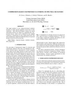
UNSUPERVISED k–WINDOWS CLUSTERING ALGORITHM For completeness purposes we outline the basic concepts of the unsupervised k-windows algorithm which is applied in this paper. This algorithm generalizes the original algorithm [15]. Suppose that we have a set of points in the Rd space. Intuitively, the k-windows algorithm tries to place a d-dimensional window (box) containing all patterns that belong to a single cluster; for all clusters present in the dataset. At first, k points are selected (possibly in a random manner). The k initial d–ranges (windows), of size a, have as centers these points. Subsequently, the patterns that lie within each d-range are identified. Next, the mean of the patterns that lie within each d–range (i.e. the mean value of the d–dimensional points) is calculated. The new position of the d–range is such that its center coincides with the previously computed mean value. The last two steps are repeatedly executed as long as the increase in the number of patterns included in the d–range that results from this motion satisfies a stopping criterion. The stopping criterion is determined by a variability threshold θv that corresponds to the least change in the center of a d–range that is acceptable to recenter the d–range. This process is illustrated in Figure 1.

M1 M2 M3

Figure 1: Sequential Movements (solid lines) of the initial window M 1 that result to the final window M 3. Once movement is terminated, the d–ranges are enlarged in order to capture as many patterns as possible from the cluster. Enlargement takes place at each dimension separately. The d–ranges are enlarged by θ e /l percent at each dimension, where θe is user defined, and l stands for the number of previous successful enlargements. After the enlargement in one dimension is performed, the window is moved, as described above. Once movement terminates, the proportional increase in the number of patterns included in the window is calculated. If this proportion does not exceed the user–defined coverage threshold, θc , the enlargement and movement steps are rejected and the position and size of the d–range are reverted to their prior to enlargement values. Otherwise, the new size and position are accepted. If enlargement is accepted for dimension d 0 > 2, then for all dimensions d00 , such that d00 < d0 , the enlargement process is performed again assuming as initial position the current position of the window. This process terminates if enlargement in any dimension does not result in a proportional increase in the number of patterns included in the window beyond the threshold θc . An example of this process is provided in Figure 2. In the figure the window is initially enlarged horizontally (E1). This enlargement is rejected since it does not produce an increase in the number of patterns included. Next the window is enlarged vertically, this enlargement is accepted, and the result of the subsequent movements and

E1

E2

Figure 2: The enlargement process. Enlargement in the horizontal dimension (E1) is rejected, while in the vertical dimension it is accepted. After subsequent movements and enlargements the window becomes E2. Further enlargement in the horizontal dimension is rejected.

enlargements is the initial window to become E2. Next enlargement in the horizontal direction is reconsidered but it is rejected again. The key idea to automatically determine the number of clusters, is to apply the k-windows algorithm using a sufficiently large number of initial windows. The windowing technique of the k-windows algorithm allows for a large number of initial windows to be examined, without any significant overhead in time complexity. Once all the processes of movement and enlargement for all windows are terminates, all overlapping windows are considered for merging. The merge operation is guided by a merge threshold θ m . Having identified two overlapping windows, the number of patterns that lie in their intersection is calculated. Next the proportion of this number to the total patterns included in each window is calculated. If the mean of these two proportions exceeds θm , then the windows are considered to belong to a single cluster and are merged, otherwise not. This operation is illustrated in Figure 3; the extent of overlapping between windows W 1 and W2 exceeds the threshold criterion and the algorithm considers both to belong to a single cluster, unlike windows W 3 and W4 , which capture two different clusters.

W1

W3

W2

W4

Figure 3: The merging procedure. W1 and W2 have many points in common thus they are considered to belong to the same cluster. On the other hand W3 and W4 , capture two different clusters. The remaining windows, after the quality of the partition criterion is met, define the final set of clusters. If the quality of a partition, determined by the number of patterns contained in any window, with respect to all patterns is not the desired one, the algorithm is re-executed. The user defined parameter u serves this purpose. Thus the algorithm takes as input seven user defined parameters: 1. 2. 3. 4. 5. 6. 7.

a: the initial window size, u: the quality parameter, θe : the enlarge threshold, θm : the merge threshold, θc : the coverage threshold, θv : the variability threshold k: the number of initial windows

The output of the algorithm is a number of sets that define the final clusters discovered in the original dataset. In brief, the algorithm works as follows: 1. 2. 3. 4. 5.

input{a, u, θe , θm , θc , θv } Determine the number, k, and the centers of the initial d–ranges. Perform sequential movements and enlargements of the d–ranges. Perform the merging of the resulting d–ranges. Report the groups of d–ranges that comprise the final clusters.

THE ALGORITHMIC COMPLEXITY OF k-WINDOWS ALGORITHM The most demanding step of the algorithm in terms of computational time is the identification of the patterns of the dataset that lie within a specific d–range (Orthogonal Range Search Problem). To make this step time efficient a technique from Computational Geometry [17, 18, 19, 20] is employed. This technique constructs a multi–dimensional binary tree for the data at a preprocessing step and traverses this tree to solve the Orthogonal Range Search Problem.

Figure 4: A set V = {p1 , p2 , . . . , p16 } of points in 2-dimensional space R2 and the corresponding 2-dimensional binary tree. From the performance viewpoint, the multi–dimensional binary tree requires, optimally, θ(dn) storage and can be optimally constructed in θ(dn log n) time, where d is the dimension of the data and n is the number of patterns. The worst–case behavior of the query time is O(|A| + dn1−1/d ) (see [20]) where A is the set containing the points belonging to the specific d–range. In the original paper [15] for the k-windows algorithm, a different type of data structure was used. Instead of a multi–dimensional binary tree, a range tree was constructed. Despite the fact that search in a range tree has a polylogarithmic time complexity; the storage requirement is super–linear with respect to the dimensionality d of the data. Thus, in [21], the multi–dimensional binary tree version was proposed to render the algorithm more suitable to real–life problems. In the version of the algorithm proposed in this paper a range tree is constructed only for the first coordinate of the data. This tree is solely used to select the initial window positions. As previously mentioned the user is given the option to select the number of d–ranges employed by the algorithm. More specifically, the user by choosing the value i, initializes 2i , d–ranges. The algorithm goes to depth i of the range tree which has 2i nodes. From each node at depth i a single point is selected to comprise the center of one window. For each

node that lies to the left of the middle node the point at the leftmost leaf of the subtree with root that node is selected. Respectively, for each node that lies to the right of the middle node, the point at the rightmost leaf of the subtree with root that node, is selected. Although different methods can also be used we chose this approach because it takes into account from the beginning the structure of the data.

EXPERIMENTAL RESULTS To investigate the performance of the k-windows algorithm in gene expression microarray data we used data from a previous study that examined mRNA expression profiles from 72 leukemia patients to develop an expressionbased classification method for acute leukemia [4]. Affymetrix Hu6800 GeneChips were used in that study. This data set contains a large number of patients and has been well characterized. Each sample is measured over 7129 genes. The first 38 samples have been used for the clustering process (train set), while the remaining 34 were used to evaluate the final clusters (test set). The initial 38 samples contained 27 acute myeloid leukemia (ALL) samples and 11 acute lymphoblastic leukemia (AML) samples. The test set contained 20 ALL samples and 14 AML samples. Golub et al. in [4] applied the Self Organizing Map [22] (SOM) clustering algorithm on the training set, selecting 50 highly correlated genes with the ALL-AML class distinction. SOM automatically grouped the 38 samples into two classes with one containing 24 out of the 25 ALL samples and the other contained 10 out of the 13 AML samples. Generally, in a typical biological system, it is often not known how many genes are sufficient to characterize a macroscopic phenotype. In practice, a working mechanistic hypothesis that is testable and largely captures the biological truth seldom involves more than a few dozens of genes, and knowing the identity of these relevant genes is very important [23]. Initially we applied the k-windows algorithm over the train set using all 7129 genes as well as various randomly selected gene collections ranging from 10 to 2000. The algorithm produced clusters that often contained both AML and ALL samples. Typically, at least 80% of all the samples that were assigned to a cluster were characterized by the same leukemia type. To improve the quality of the clustering, it proved essential to identify genes that significantly contribute to the partition of interest. Thus we selected the 50 most highly correlated genes with the ALL-AML class distinction (top 25 differentially expressed probe sets in either sample group) according to Thomas et al. [24]. More specifically their approach is based on well-defined assumptions, uses rigorous and well-characterized statistical measures, and accounts for the heterogeneity and genomic complexity of the data. The modeling approach uses known sample group membership to focus on expression profiles of individual genes in a sensitive and robust manner, and can be used to test statistical hypotheses about gene expression. The first step in the statistical analysis of microarray expression profiles is preprocessing and/or transformation of the data. This includes removal of the spiked oligonucleotide controls. The second step is to estimate correction factors for sample-specific heterogeneity, as well as for chip-specific heterogeneity, and to use these factors to normalize the data. The final step is to perform a regression analysis to estimate the relevant model parameters for each gene transcript using robust statistical techniques in order to assess the confidence level that the corresponding gene is differentially expressed between the two groups. Applying the k-windows algorithm for those 50 genes over the train set produced 6 clusters each of which contained samples from either ALL or AML, as exhibited in Table I. In particular, 4 clusters contained only ALL samples and 2 clusters contained only AML samples. Leukemia type ALL AML

Cluster 1 10 0

ALL Clusters Cluster 2 Cluster 3 3 10 0 0

Cluster 4 4 0

AML Clusters Cluster 1 Cluster 2 0 0 8 3

Table I: Clustering result for the train set To evaluate the clustering result each sample from the test set was assigned to one of the clusters discovered in the train set according to its distance from the cluster center. Specifically, if an ALL (AML) sample from the test set was assigned to an ALL (AML, respectively) cluster then that sample was considered correctly classified. From the results exhibited in Table II, it is evident that only 3 AML samples from the test set were misclassified, resulting in a 91.2% correct classification.

Leukemia type ALL AML

Cluster 1 8 0

ALL Clusters Cluster 2 Cluster 3 0 9 0 3

Cluster 4 3 0

AML Clusters Cluster 1 Cluster 2 0 0 8 3

Table II: Clustering result for the test set

CONCLUDING REMARKS In this contribution we present a modification of the recently proposed k-windows clustering algorithm. Cluster analysis presented here groups leukemia samples into clusters based on similar gene expression microarray data. The data set used was provided by The Center of Genome Research, Whitehead Institute [4]. From the 7129 genes provided, 50 of them (top 25 differentially expressed probe sets in either sample group) were used according to the modeling approach of [24]. This approach makes no distributional assumptions, it is well-founded, and provides a sensitive and robust method to extract relevant information from DNA microarrays. Our analysis produced 6 different clusters, each one containing only AML or ALL samples. These clusters were evaluated using an independent test set, exhibiting high classification success.

ACKNOWLEDGMENT The authors thank T.R. Golub and his colleagues at MIT for making their AML/ALL data set available in the public domain as well as the referees for their valuable suggestions and comments. The authors also ackowledge the support of the “Karatheodoris” research grant awarded by the Research Committee of the University of Patras, and the “Pythagoras” research grant awarded by the Greek Ministry of Education and Religious Affairs and the European Union.

REFERENCES [1] D. Jiang; C. Tang; A. Zhangi, to appear, “Cluster analysis for gene expression data: A survey”, IEEE Transactions on Knowledge and Data Engineering. [2] M.B. Eisen; P.T. Spellman; P.O. Brown; D. Botstein, 1998, “Cluster analysis and display of genome-wide expression patterns”, Proc. Natl. Acad. Sci. USA, 95, pp. 14863–14868. [3] X. Wen; S. Fuhrman; G. Michaels; D. Carr; S. Smith; J. Barker; R. Somogyi, 1998, “Large-scale temporal gene expression mapping of cns development”, Proceedings of the National Academy of Science USA, 95, pp. 334–339. [4] T.R. Golub; D.K Slomin; P. Tamayo; C. Huard; M. Gaasenbeek; J. Mesirov; H. Coller; M.L. Loh; J. Downing; M. Caligiuri; C. Bloomfield; E. Lander, 1999, “Molecular classification of cancer: Class discovery and class prediction by gene expression monitoring”, Science, 286, pp. 531–537. [5] T. Hastie; R. Tibshirani; J. Friedman, 2001, “The elements of statistical learning”, Springer-Verlag. [6] U.M. Fayyad; G. Piatetsky-Shapiro; P. Smyth, 1996, “Advances in knowledge discovery and data mining”, MIT Press. [7] M.S. Aldenderfer; R.K. Blashfield, 1984, “Cluster analysis”, volume 44 of Quantitative Applications in the Social Sciences, SAGE Publications, London. [8] V. Ramasubramanian; K. Paliwal, 1992, “Fast k-dimensional tree algorithms for nearest neighbor search with application to vector quantization encoding”, IEEE Transactions on Signal Processing, 40(3), pp. 518– 531. [9] R.W. Becker; G.V. Lago, 1970, “A global optimization algorithm”, In Proceedings of the 8th Allerton Conference on Circuits and Systems Theory, pp. 3–12. [10] A. Torn; A. Zilinskas, 1989, “Global optimization”, Springer-Verlag, Berlin.

[11] U. Alon; N. Barkai; D.A. Notterman; K.Gish; S. Ybarra; D. Mack; A.J. Levine, 1999, “Broad patterns of gene expression revealed by clustering analysis of tumor and normal colon tissues probed by oligonucleotide array”, Proc. Natl. Acad. Sci. USA, 96(12), pp. 6745–6750. [12] R. Shamir; R. Sharan, 2000, “Click: A clustering algorithm for gene expression analysis”, In 8th International Conference on Intelligent Systems for Molecular Biology (ISMB 00). AAAIPress. [13] S. Tavazoie; J.D. Hughes; M.J. Campbell; R.J. Cho; G.M. Church, 1999, “Systematic determination of genetic network architecture”, Nature genetics, volume 22, pp. 281–285. [14] J.A. Hartigan; M.A. Wong, 1979, “A k-means clustering algorithm”, Applied Statistics, 28, pp. 100–108. [15] M.N. Vrahatis; B. Boutsinas; P. Alevizos; G. Pavlides, 2002, “The new k-windows algorithm for improving the k-means clustering algorithm”, Journal of Complexity, 18, pp. 375–391. [16] D.K. Tasoulis; M.N. Vrahatis, 2004, “Unsupervised distributed clustering”, In Proceedings of the IASTED International Conference on Parallel and Distributed Computing and Networks. Innsbruck, Austria. [17] P. Alevizos, 1998, “An algorithm for orthogonal range search in d > 3 dimensions”, In Proceedings of the 14th European Workshop on Computational Geometry. Barcelona. [18] B. Chazelle, 1986, “Filtering search: A new approach to query-answering”, SIAM J. Comput, 15(3), pp. 703–724. [19] B. Chazelle; L.J. Guibas, 1986, “Fractional cascading II: Applications”, Algorithmica, 1, pp. 163–191. [20] F. Preparata; M. Shamos, 1985, “Computational geometry”, Springer Verlag, New York, Berlin. [21] P. Alevizos; B. Boutsinas; D.K. Tasoulis; M.N. Vrahatis, 2002, “Improving the orthogonal range search k-windows clustering algorithm”, In Proceedings of the 14th IEEE International Conference on Tools with Artificial Intelligence, pp. 239–245. Washington, D.C. [22] T. Kohonen, 1997, “Self–organized maps”, Springer Verlag, New York, Berlin. [23] E.P. Xing; R.M. Karp, 2001, “Cliff: Clustering of high–dimensional microarray data via iterative feature filtering using normalized cuts”, Bioinformatics Discovery Note, 1, pp. 1–9. [24] J.G. Thomas; J.M. Olson; S.J. Tapscott; L.P. Zhao, 2001, “An efficient and robust statistical modeling approach to discover differentially expressed genes using genomic expression profiles”, Genome Research, 11, pp. 1227–1236.