delivery. Applications such as Internet streaming, wireless videophones, .... algorithm. When a standards compliant encoder is assumed, the low- resolution ..... rates of practical interest, and it is most bothersome as the bit-rate decreases.
Chapter 11 Super-resolution from compressed video C. Andrew Segall1, Aggelos K. Katsaggelos1, Rafael Molina2, and Javier Mateos2 1
Department of Electrical and Computer Engineering Northwestern University Evanston, IL 60208-3118 {asegall,aggk}@ece.nwu.edu
2
Departamento de Ciencias de la Computación e I.A. Universidad de Granada 18071 Granada, Spain {rms,jmd}@decsai.ugr.es
Abstract:
The problem of recovering a high-resolution frame from a sequence of low-resolution and compressed images is considered. The presence of the compression system complicates the recovery problem, as the operation reduces the amount of frequency aliasing in the low-resolution frames and introduces a non-linear noise process. Increasing the resolution of the decoded frames can still be addressed in a recovery framework though, but the method must also include knowledge of the underlying compression system. Furthermore, improving the spatial resolution of the decoded sequence is no longer the only goal of the recovery algorithm. Instead, the technique is also required to attenuate compression artifacts.
Key words:
super-resolution, post-processing, image scaling, resolution enhancement, interpolation, spatial scalability, standards conversion, de-interlacing, video compression, image compression, motion vector constraint
1.
INTRODUCTION
Compressed video is rapidly becoming the preferred method for video delivery. Applications such as Internet streaming, wireless videophones, 1
2
Chapter 11
DVD players and HDTV devices all rely on compression techniques, and each requires a significant amount of data reduction for commercial viability. To introduce this reduction, a specific application often employs a low-resolution sensor or sub-samples the original image sequence. The reduced resolution sequence is then compressed in a lossy manner, which produces an estimate of the low-resolution data. For many tasks, the initial reconstruction of the compressed sequence is acceptable for viewing. However, when an application requires a high-resolution frame or image sequence, a super-resolution algorithm must be employed. Super-resolution algorithms recover information about the original highresolution image by exploiting sub-pixel shifts in the low-resolution data. These shifts are introduced by motion in the sequence and make it possible to observe samples from the high-resolution image that may not appear in a single low-resolution frame. Unfortunately, lossy encoding introduces several distortions that complicate the super-resolution problem. For example, most compression algorithms divide the original image into blocks that are processed independently. At high compression ratios, the boundaries between the blocks become visible and lead to “blocking” artifacts. If the coding errors are not removed, super-resolution techniques may produce a poor estimate of the high-resolution sequence, as coding artifacts may still appear in the high-resolution result. Additionally, the noise appearing in the decoded images may severely affect the quality of any of the motion estimation procedures required for resolution enhancement. A straightforward solution to the problem of coding artifacts is to suppress any errors before resolution enhancement. The approach is appealing, as many methods for artifact removal are presented in the literature [1]. However, the sequential application of one of these postprocessing algorithms followed by a super-resolution technique rarely provides a good result. This is caused by the fact that information removed during post-processing might be useful for resolution enhancement. The formulation of a recovery technique that incorporates the tasks of post-processing and super-resolution is a natural approach to be followed. Several authors have considered such a framework, and a goal of this chapter is to review relevant work. Discussion begins in the next section, where background is presented on the general structure of a hybrid motion compensation and transform encoder. In Section 3, super-resolution methods are reviewed that derive fidelity constraints from the compressed bit-stream. In Section 4, work in the area of compression artifact removal is surveyed. Finally, a general framework for the super-resolution problem is proposed in Section 5. The result is a super-resolution algorithm for compressed video.
11. Super-resolution from compressed video
2.
3
VIDEO COMPRESSION BASICS
The purpose of any image compression algorithm is to decrease the number of bits required to represent a signal. Loss-less techniques can always be employed. However for significant compression, information must be removed from the original image data. Many possible approaches are developed in the literature to intelligently remove perceptually unimportant content, and while every algorithm has its own nuances, most can be viewed as a three-step procedure. First, the intensities of the original images are transformed with a de-correlating operator. Then, the transform coefficients are quantized. Finally, the quantized coefficients are entropy encoded. The choice of the transform operator and quantization strategy are differentiating factors between techniques, and examples of popular operators include wavelets, Karhunen-Loeve decompositions and the Discrete Cosine Transform (DCT) [2]. Alternatively, both the transform and quantization operators can be incorporated into a single operation, which results in the technique of vector quantization [3]. The general approach for transform coding an MxN pixel image is therefore expressed as x = Q[Tg],
(11.1)
where g is an (MN)x1 vector containing the ordered image, T is an (MN)x(MN) transformation matrix, Q is a quantization operator, and x is an (MN)x1 vector that contains the quantized coefficients. The quantized transform coefficients are then encoded with a loss-less technique and sent to the decoder. At the standard decoder, the quantized information is extracted from any loss-less encoding. Then, an estimate of the original image is generated according to
gˆ = T −1Q * [x],
(11.2)
where g^ is the estimate of the original image, T-1 is the inverse of the transform operator, and Q* represents a de-quantization operator. Note that the purpose of the de-quantization operator is to map the quantized values in x to transform coefficients. However, since the original quantization operator Q is a lossy procedure, this does not completely undo the information loss and Q*[Q[x]] x. The compression method described in (11.1) and (11.2) forms the foundation for current transform-based compression algorithms. For example, the JPEG standard divides the original image into 8x8 blocks and
4
Chapter 11
transforms each block with the DCT [4]. The transform coefficients are then quantized with a perceptually weighted method, which coarsely represents high-frequency information while maintaining low-frequency components. Next, the quantized values are entropy encoded and passed to the decoder, where multiplying the transmitted coefficients by the quantization matrix and computing the inverse-DCT reconstructs the image. While transform coding provides a general method for two-dimensional image compression, its extension to video sequences is not always practical. As one approach, a video sequence might be encoded as a sequence of individual images. (If JPEG is utilized, this is referred to as motion-JPEG.) Each image is compressed with the transform method of (11.1), sent to a decoder, and then reassembled into a video sequence. Such a method clearly ignores the temporal redundancies between image frames. If exploited, these redundancies lead to further compression efficiencies. One way to capitalize on these redundancies is to employ a three-dimensional transform encoder [5, 6]. With such an approach, several frames of an image sequence are processed simultaneously with a three-dimensional transform operator. Then, the coefficients are quantized and sent to the decoder, where the group of frames is reconstructed. To realize significant compression efficiencies though, a large number of frames must be included in the transform. This precludes any application that is sensitive to the delay of the system. A viable alternative to multi-dimensional transform coding is the hybrid technique of motion compensation and transform coding [7]. In this method, images are first predicted from previously decoded frames through the use of motion vectors. The motion vectors establish a mapping between the frame being encoded and previously reconstructed data. Using this mapping, the difference between the original image and its estimate can be calculated. The difference, or error residual, is then passed to a transform encoder and quantized. The entire procedure is expressed as
[(
x = Q T g − gˆ MC
)] ,
(11.3)
where x is the quantized transform coefficients, and g^ MC is the motion compensated estimate of g that is predicted from previously decoded data. To decode the result, the quantized transform coefficients and motion vectors are transmitted to the decoder. At the decoder, an approximation of the original image is formed with a two-step procedure. First, the motion vectors are utilized to reconstruct the estimate. Then, the estimate is refined with the transmitted error residual. The entire procedure is express as
gˆ = T −1Q * [x] + gˆ MC ,
(11.4)
11. Super-resolution from compressed video
5
where g^ is the decoded image, g^ MC is uniquely defined by the motion vectors, and Q* is the de-quantization operator. The combination of motion compensation and transform coding provides a very practical compression algorithm. By exploiting the temporal correlation between frames, the hybrid method provides higher compression ratios than encoding every frame individually. In addition, compression gains do not have to come with an explicit introduction of delay. Instead, motion vectors can be restricted to only reference previous frames in the sequence, which allows each image to be encoded as it becomes available to the encoder. When a slight delay is acceptable though, more sophisticated motion compensation schemes can be employed that utilize future frames for a bi-directional motion estimate [8]. The utility of motion estimation and transform coding makes it the backbone of current video-coding standards. These standards include MPEG-1, MPEG-2, MPEG-4, H.261 and H.263 [9-14]. In each of the methods, the original image is first divided into blocks. The blocks are then encoded using one of two available methods. For an intra-coded block, the block is transformed by the DCT and quantized. For inter-coded blocks, motion vectors are first found to estimate the current block from previously decoded images. This estimate is then subtracted from the current block, and the residual is transformed and quantized. The quantization and motion vector data is sent to the decoder, which estimates the original image from the transmitted coefficients. The major difference between the standards lies in the representation of the motion vectors and quantizers. For example, motion vectors are signaled at different resolutions in the standards. In H.261, a motion vector is represented with an integer number of pixels. This is different from the methods employed for MPEG-1, MPEG-2 and H.263, where the motion vectors are sent with half-pixel accuracy and an interpolation procedure is defined for the estimate. MPEG-4 utilizes more a sophisticated method for representing the motion, which facilitates the transmission of motion vectors at quarter-pixel resolution. Other differences also exist between the standards. For example, some standards utilize multiple reference frames or multiple motion vectors for the motion compensated prediction. In addition, the structure and variability of the quantizer is also different. Nevertheless, for the purposes of developing a super-resolution algorithm, it is sufficient to remember that quantization and motion estimation data will always be provided in the bit-stream. When a portion of a sequence is intra-coded, the quantizer and transform operators will express information about the intensities of the original image. When blocks are inter-coded, motion vectors will provide an (often crude) estimate of the motion field.
6
3.
Chapter 11
INCORPORATING THE BIT-STREAM
With a general understanding of the video compression process, it is now possible to incorporate information from a compressed bit-stream into a super-resolution algorithm. Several methods for utilizing this information have been presented in the literature, and a survey of these techniques is presented in this section. At the high-level, these methods can be classified according to the information extracted from the bit-stream. The first class of algorithms incorporates the quantization information into the resolution enhancement procedure. This data is transmitted to the decoder as a series of indices and quantization factors. The second class of algorithms incorporates the motion vectors into the super-resolution algorithm. These vectors appear as offsets between the current image and previous reconstructions and provide a degraded observation of the original motion field.
3.1
System Model
Before incorporating parameters from the bit-stream into a superresolution algorithm, a definition of the system model is necessary. This model is utilized in all of the proposed methods, and it relates the original high-resolution images to the decoded low-resolution image sequence. Derivation of the model begins by generating an intermediate image sequence according to
g = AHf ,
(11.5)
where f is a (PMPN)x1 vector that represents a (PM)x(PN) high-resolution image, g is an (MN)x1 vector that contains the low-resolution data, A is an (MN)x(PMPN) matrix that realizes a sub-sampling operation and H is a (PMPN)x(PMPN) filtering matrix. The low-resolution images are then encoded with a video compression algorithm. When a standards compliant encoder is assumed, the lowresolution images are processed according to (11.3) and (11.4). Incorporating the relationship between low and high-resolution data in (11.5), the compressed observation becomes
[ [
(
−1 Q * Q TDCT AHf − gˆ MC gˆ = TDCT
)] ] + gˆ
MC
,
(11.6)
-1 where g^ is the decoded low-resolution image, TDCT and TDCT are the forward * and inverse DCT operators, respectively, Q and Q are the quantization and
11. Super-resolution from compressed video
7
de-quantization operators, respectively, and g^ MC is the temporal prediction of the current frame based on the motion vectors. If a portion of the image is encoded without motion compensation (i.e. intra-blocks), then the predicted values for that region are zero. Equation (11.6) defines the relationship between a high-resolution frame and a compressed frame for a given time instance. Now, the high-resolution frames of a dynamic image sequence are also coupled through the motion field according to
f l = Cl ,k f k ,
(11.7)
where fl and fk are (PMPN)x1 vectors that denote the high-resolution data at times l and k, respectively, and Cl,k is a (PMPN)x(PMPN) matrix that describes the motion vectors relating the pixels at time k to the pixels at time l. These motion vectors describe the actual displacement between highresolution frames, which should not be confused with the motion information appearing in the bit-stream. For regions of the image that are occluded or contain objects entering the scene, the motion vectors are not defined. Combining (11.6) and (11.7) produces the relationship between a highresolution and compressed image sequence at different time instances. This relationship is given by
[ [
(
−1 Q * Q TDCT AHCl , k f k − gˆ MC gˆ l = TDCT l
)] ] + gˆ
MC , l
(11.8)
where g^ l is the compressed frame at time l and g^ lMC is the motion compensated prediction utilized in generating the compressed observation.
3.2
Quantizers
To explore the quantization information that is provided in the bit-stream, researchers represent the quantization procedure with an additive noise process according to
[ [
(
−1 Q * Q TDCT AHC l ,k f k − gˆ lMC TDCT
)] ]
= AHC l ,k f k − gˆ MC + n Ql , (11.9) l
where nlQ represents the quantization noise at time l. The advantage of this representation is that the motion compensated estimates are eliminated from the system model, which leads to super-resolution methods that are independent of the underlying motion compensation scheme. Substituting
8
Chapter 11
(11.9) into (11.8), the relationship between a high-resolution image and the low-resolution observation becomes
gˆ l = AHC l ,k f k + n Ql ,
(11.10)
where the motion compensated estimates in (11.8) cancel out. With the quantization procedure represented as a noise process, a single question remains: What is the structure of the noise? To understand the answers proposed in the literature, the quantization procedure must first be understood. In standards based compression algorithms, quantization is realized by dividing each transform coefficient by a quantization factor. The result is then rounded to the nearest integer. Rounding discards data from the original image sequence, and it is the sole contributor to the noise term of (11.10). After rounding, the encoder transmits the integer index and the quantization factor to the decoder. The transform coefficient is then reconstructed by multiplying the two transmitted values, that is T (g, i ) , TDCT (gˆ , i ) = q (i )x(i ) = q(i )⋅ Round DCT q (i )
(11.11)
^ where TDCT(g,i) and TDCT( g,i) denote the ith transform coefficient of the low^ resolution image g and the decoded estimate g, respectively, q(i) is the quantization factor and x(i) is the index transmitted by the encoder for the ith transform coefficient, and Round(· ) is an operator that maps each value to the nearest integer. Equation (11.11) defines a mapping between each transform coefficient and the nearest multiple of the quantization factor. This provides a key constraint, as it limits the quantization error to half of the quantization factor. With knowledge of the quantization error bounds, a set-theoretic approach to the super-resolution problem is explored in [15]. The method restricts the DCT coefficients of the solution to be within the uncertainty range signaled by the encoder. The process begins by defining the constraint set
(
)
q q fˆk ∈ fˆk : − l ≤ TDCT AHC l , k fˆk − gˆ l ≤ l , 2 2
(11.12)
where f^k is the high-resolution estimate, ql is a vector that contains the quantization factors for time l, g^ l is estimated by choosing transform coefficients centered on each quantization interval, and the less-than operator is defined on an element by element basis. Finding a solution that
11. Super-resolution from compressed video
9
satisfies (11.12) is then accomplished with a Projection onto Convex Sets (POCS) iteration, where the projection of f^k onto the set is defined as −1 C Tl ,k H T A T TDCT ˆ f k − T T T −1 Pl fˆk = ˆ − C l ,k H A TDCT f k ˆ f k ,
[]
{T
},
ˆ − (T gˆ + .5q ) DCT l l
DCT AHCl , k f k
TDCT AHC l ,k
2
(
)
TDCT AHC l ,k fˆk − gˆ l > .5q l
{T
},
ˆ − (T gˆ − .5q ) DCT l l
DCT AHCl , k f k
TDCT AHC l ,k
2
(
)
TDCT AHCl , k fˆk − gˆ l < −.5q l otherwise (11.13)
where Pl[f^k] is the projection operator that accounts for the influence of the observation g^ l on the estimate of the high-resolution image f^k. The set-theoretic method is well suited for limiting the magnitude of the quantization errors in a system model. However, the projection operator does not encapsulate any additional information about the shape of the noise process within the bounded range. When information about the structure of the noise is available, then an alternative description may be more appropriate. One possible method is to utilize probabilistic descriptions of the quantization noise in the transform domain and rely on maximum a posteriori or maximum likelihood estimates for the high-resolution image. This approach is considered in [16], where the quantization noise is represented with the density
( )= (
pN n Qk
pN TDCT n Qk −1 TDCT
),
(11.14)
-1 where nkQ is the quantization noise in the spatial domain, |TDCT | is the determinant of the transform operator, and pN(· ) and pN-(· ) denote the probability density functions in the spatial and transform domains, respectively [17]. Finding a simple expression for the quantization noise in the spatial domain is often difficult, and numerical solutions are employed in [16]. However, an important case is considered in [18, 19], where the quantization noise is expressed with the Gaussian distribution
10
Chapter 11
( )
( )(
)( )
T −1 1 −1 p N n Qk = Z exp − n Qk TDCT K Qk TDCT (11.15) n kQ , 2 _ where KkQ is the covariance matrix of the quantization noise in the transform domain for the kth frame of the sequence, and Z is a normalizing constant. Several observations pertaining to (11.15) are appropriate. First, notice that if the distributions for the quantization noise in the transform domain are independent and identically distributed, then pN(nkQ) is spatially uncorrelated and identically distributed. This arises from the structure of the DCT and is representative of the flat quantization matrices typically used for intercoding. As a second observation, consider the perceptually weighted quantizers that are utilized for intra-coding. In this quantization strategy, high-frequency coefficients are represented with less fidelity. Thus, the distribution of the noise in the DCT domain depends on the frequency. When the quantization noise is independent in the transform domain, then pN(nkQ) will be spatially correlated. Incorporating the quantizer information into a super-resolution algorithm should improve the results, as it equips the procedure with knowledge of the non-linear quantization process. In this section, three approaches to utilizing the quantizer data have been considered. The first method enforces bounds on the quantization noise, while the other methods employ a probabilistic description of the noise process. Now that the proposed methods have been presented, the second component of incorporating the bit-stream can be considered. In the next sub-section, methods that utilize the motion vectors are presented.
3.3
Motion Vectors
Incorporating the motion vectors into the resolution enhancement algorithm is also an important problem. Super-resolution techniques rely on sub-pixel relationships between frames in an image sequence. This requires a precise estimate of the actual motion, which has to be derived from the observed low-resolution images. When a compressed bit-stream is available though, the transmitted motion vectors provide additional information about the underlying motion. These vectors represent a degraded observation of the actual motion field and are generated by a motion estimation algorithm within the encoder. Several traits of the transmitted motion vectors make them less than ideal for representing actual scene motion. As a primary flaw, motion vectors are not estimated at the encoder by utilizing the original low-resolution frames. Instead, motion vectors establish a correspondence between the current low resolution frame and compressed frames at other time instances. When the
11. Super-resolution from compressed video
11
compressed frames represent the original image accurately, then the correlation between the motion vectors and actual motion field is high. As the quality of compressed frames decreases, the usefulness of the motion vectors for estimating the actual motion field is diminished. Other flaws also degrade the compressed observation of the motion field. For example, motion estimation is a computationally demanding procedure. When operating under time or resource constraints, an encoder often employs efficient estimation techniques. These techniques reduce the complexity of the algorithm but also decrease the reliability of the motion vectors. As a second problem, motion vectors are transmitted with a relatively coarse sampling. At best, one motion vector is assigned to every 8x8 block in a standards compliant bit-stream. Super-resolution algorithms, however, require a much denser representation of motion. Even with the inherent errors in the transmitted motion vectors, methods have been proposed that capitalize on the transmitted information. As a first approach, a super-resolution algorithm that estimates the motion field by refining the transmitted data is proposed in [18, 19]. This is realized by initializing a motion estimation algorithm with the transmitted motion vectors. Then, the best match between decoded images is found within a small region surrounding each initial value. With the technique, restricting the motion estimate adds robustness to the search procedure. More importantly, the use of a small search area greatly reduces the computational requirements of the motion estimation method. A second proposal does not restrict the motion vector search [20, 21]. Instead, the motion field can contain a large deviation from the transmitted data. In the approach, a similarity measure between each candidate solution and the transmitted motion vector is defined. Then, motion estimation is employed to minimize a modified cost function. Using the Euclidean distance as an example of similarity, the procedure is expressed as ˆ = arg min AHC fˆ − gˆ C l ,k l,k k l C l ,k
2
+λ
MN −1
∑ i =0
(
T ,i cl , k (i ) − AMV ClEncoder ,k
)
2
, (11.16)
^ where C l,k is a matrix that represents the estimated motion field, cl,k (i) is a two-dimensional vector the contains the motion vector for pixel location i, Cl,kEncoder is a matrix that contains the motion vectors provided by the encoder, ATMV (Cl,kEncoder,i) produces an estimate for the motion at pixel location i from quantifies the confidence in the the transmitted motion vectors, and transmitted information. In either of the proposed methods, an obstacle to incorporating the transmitted motion vectors occurs when motion information is not provided
12
Chapter 11
for the frames of interest. In some cases, such as intra-coded regions, the absence of motion vectors may indicate an occlusion. In most scenarios though, the motion information is simply being signaled in an indirect way. For example, an encoder may provide the motion estimates Cl,l'Encoder and Cl',kEncoder , while not explicitly transmitting Cl,kEncoder . When a super-resolution ^ Encoder algorithm needs to estimate C from l,k , the method must determine Cl,k the transmitted information. For vectors with pixel resolution, a straightforward approach is to add the horizontal and vertical motion components to find the mapping Cl,kEncoder . The confidence in the estimate must also be adjusted, as adding the transmitted motion vectors increases the uncertainty of the estimate. In the method of [18, 19], a lower confidence in Cl,kEncoder results in a larger search area when finding the estimated motion field. In [20, 21], the decreased confidence results in smaller values for .
4.
COMPRESSION ARTIFACTS
Exploring the influence of the quantizers and motion vectors is the first step in developing a super-resolution algorithm for compressed video. These parameters convey important information about the original image sequence, and each is well suited for restricting the solution space of a high-resolution estimate. Unfortunately, knowledge of the compressed bit-stream does not address the removal of compression artifacts. Artifacts are introduced by the structure of an encoder and must also be considered when developing a super-resolution algorithm. In this section, an overview of post-processing methods is presented. These techniques attenuate compression artifacts in the decoded image and are an important component of any super-resolution algorithm for compressed video. In the next sub-section, an introduction to various compression artifacts is presented. Then, three techniques for attenuating compression artifacts are discussed.
4.1
Artifact Types
Several artifacts are commonly identified in video coding. A first example is blocking. This artifact is objectionable and annoying at all bitrates of practical interest, and it is most bothersome as the bit-rate decreases. In a standards based system, blocking is introduced by the structure of the encoder. Images are divided into equally sized blocks and transformed with a de-correlating operator. When the transform considers each block independently, pixels outside of the block region are ignored and the continuity across boundaries is not captured. This is perceived as a
11. Super-resolution from compressed video
13
synthetic, grid-like error at the decoder, and sharp discontinuities appear between blocks in smoothly varying regions. Blocking errors are also introduced by poor quantization decisions. Compression standards do not define a strategy for allocating bits within a bit-stream. Instead, the system designer has complete control. This allows for the development of encoders for a wide variety of applications, but it also leads to artifacts. As an example, resource critical applications typically rely on heuristic allocation strategies. Very often different quantizers may be assigned to neighboring regions even though they have similar visual content. The result is an artificial boundary in the decoded sequence. Other artifacts are also attributed to the improper allocation of bits. In satisfying delay constraints, encoders operate without knowledge of future sequence activity. Thus, bits are distributed on an assumption of future content. When the assumption is invalid, an encoder must quickly adjust the amount of quantization to satisfy a given rate constraint. The encoded video sequence possesses a temporally varying image quality, which manifests itself as a temporal flicker. Edges and impulsive features introduce a final coding error. Represented in the frequency domain, these signals have high spatial frequency content. Quantization removes some of the information for encoding and introduces quantization error. However, when utilizing a perceptually weighted technique, additional errors appear. Low frequency data is preserved, while high frequency information is coarsely quantized. This removes the highfrequency components of the edge and introduces a strong ringing artifact at the decoder. In still images, the artifact appears as strong oscillations in the original location of the edge. Image sequences are also plagued by ringing artifacts but are usually referred to as mosquito errors.
4.2
Post-processing Methods
Post-processing methods are concerned with removing all types of coding errors and are directly applicable to the problem of super-resolution. As a general framework, post-processing algorithms attenuate compression artifacts by developing a model for spatial and temporal properties of the original image sequence. Then, post-processing techniques find a solution that satisfies the ideal properties while also remaining faithful to the available data. One approach for post-processing follows a constrained least squares (CLS) methodology [22-24]. In this technique, a penalty function is assigned to each artifact type. The post-processed image is then found by minimizing the following cost functional
14
Chapter 11 E (p ) = p − gˆ
2
+ λ1 Bp
2
+ λ 2 Rp
2
+ λ3 p − gˆ MC
2
,
(11.17)
where p is a vector representing the post-processed image, g^ is the estimate decoded from the bit-stream, B and R are matrices that penalize the appearance of blocking and ringing, respectively, g^ MC is the motion compensated prediction and 1, 2, and 3 express the relative importance of each constraint. In practice, the matrix B is implemented as a difference operator across the block boundaries, while the matrix R describes a highpass filter within each block. Finding the derivative of (11.17) with respect to p and setting it to zero represents the necessary condition for a minimum of (11.17). A solution is then found using the method of successive approximations according to
{
(
p k +1 = p k − α p k − gˆ + λ1BT Bp k + λ2 R T Rp k + λ3 p k − gˆ MC
)} , (11.18)
��������� � ����������������������� ����� ��������������� �����!������� ��"#��������������������� ��"$����� algorithm, and pk and pk+1 denote the post-processed solution at iteration k and k+1, respectively [25]. The decoded image is commonly defined as the initial estimate, p0. Then, the iteration continues until a termination criterion is satisfied. Selecting the smoothness constraints (B and R) and parameters ( 1, 2 and ) 3 defines the performance of the CLS technique, and many approaches have been developed for compression applications. As a first example, parameters can be calculated at the encoder from the intensity data of the original images, transmitted through a side channel and supplied to the postprocessing mechanism [26]. More appealing techniques vary the parameters relative to the contents of the bit-stream, incorporating the quantizer information and coding modes into the choice of parameters [27-29]. Besides the CLS approach, other recovery techniques are also suitable for post-processing. In the framework of POCS, blocking and ringing artifacts are removed by defining images sets that do not exhibit compression artifacts [30, 31]. For example, the set of images that are smooth would not contain ringing artifacts. Similarly, blocking artifacts are absent from all images with smooth block boundaries. To define the set, the amount of smoothness must be quantified. Then, the solution is constrained by
{
p ∈ g : Bg
2
}
≤ TB ,
(11.19)
where TB is the smoothness threshold used for the block boundaries and B is a difference operator between blocks.
11. Super-resolution from compressed video
15
An additional technique for post-processing relies on the Bayesian framework. In the method, a post-processed solution is computed as a maximum a posteriori (MAP) estimate of the image sequence presented to the encoder, conditioned on the observation [32, 33]. Thus, after applying Bayes’ rule, the post-processed image is given by p = arg max g
p(gˆ | p )p(p ) . p (gˆ )
(11.20)
Taking logarithms, the technique becomes p = arg max log p(gˆ | p ) + log (p ) ,
(11.21)
p
where p( g^ | p) is often assumed constant within the bounds of the quantization error. Compression artifacts are removed by selecting a distribution for the post-processed image with few compression errors. One example is the Gaussian distribution
{
p (g ) = exp − λ1 Bg
2
− λ 2 Rg
2
}.
(11.22)
In this expression, images that are likely to contain artifacts are assigned a lower probability of occurrence. This inhibits the coding errors from appearing in the post-processed solution.
5.
SUPER-RESOLUTION
Post-processing methods provide the final component of a superresolution approach. In the previous section, three techniques are presented for attenuating compression artifacts. Combining these methods with the work in Section 3 produces a complete formulation of the super-resolution problem. This is the topic of the current section, where a concise formulation for the resolution enhancement of compressed video is proposed. The method relies on the MAP estimation techniques to address compression artifacts as well as to incorporate the motion vectors and quantizer data from the compressed bit-stream.
16
Chapter 11
5.1
MAP Framework
The goal of the proposed super-resolution algorithm is to estimate the original image sequence and motion field from the observations provided by the encoder. Within the MAP framework, this joint estimate is expressed as
{ p(f , D p (G, D max
ˆ fˆk , D TB ,TF = arg max
k
f k ,DTB ,TF
= arg
f k ,DTB ,TF
TB ,TF
Encoder | G, DTB ,TF
Encoder TB ,TF
)} )p(f
| f k , DTB ,TF
Encoder p(G, D TB ,TF )
k , DTB ,TF
)
(11.23)
,
where f^k is the estimate for the high-resolution image, G is an (MN)xL matrix that contains the L compressed observations g^ k-TB ,…, g^ k+TF , TF and TB are the number of frames contributing to the estimate in the forward and backward direction of the temporal axis, respectively, and DTB,TF and DEncoder TB,TF are formed by lexicographically ordering the respective motion vectors Encoder ,…,CEncoder Ck-TB,k ,…,Ck+TF,k and Ck-TB,k k+TF,k into vectors and storing the result in a (PMPN)x(TF+TB+1) matrix. 5.1.1
Fidelity Constraints
Definitions for the conditional distributions follow from the previous sections. As a first step, it is assumed that the decoded intensity values and transmitted motion vectors are independent. This results in the conditional density
(
)
(
Encoder Encoder p G, DTB ,TF | f k , D TB ,TF = p (G | f k , DTB ,TF )p DTB ,TF | f k , D TB ,TF
). (11.24)
Information from the encoder is then included in the algorithm. The density function p(G | fk, DTB,TF) describes the noise that is introduced during quantization, and it can be derived through the mapping presented in (11.14). The corresponding conditional density is 1 k +TF (AHCl ,k f k − gˆ l )T K l−1 (AHCl ,k f k − gˆ l ) , p (G | f k , DTB ,TF ) ∝ exp − 2 l = k −TB (11.25)
∑
11. Super-resolution from compressed video
17
when g^ l is the decoded image at time instant l and Kl is the noise covariance matrix in the spatial domain that is found by modeling the noise in the transform domain as Gaussian distributed and uncorrelated. The second conditional density relates the transmitted motion vectors to the original motion field. Following the technique appearing in (11.16), an example distribution is k + TF MN −1 2 Encoder T ,i , p DTB cl , k (i ) − AMV ClEncoder ,TF | f k , DTB ,TF ∝ exp − γ ,k l = k − TB i = 0 (11.26)
(
)
∑ ∑
(
)
where cl,k(i) is the motion vector for pixel location i, ATMV (Cl,kEncoder,i) estimates the motion at pixel i from the transmitted motion vectors, and ���� � � positive value that expresses a confidence in the transmitted vectors. As a final piece of information from the decoder, bounds on the quantization error should be exploited. These bounds are known in the transform domain and express the maximum difference between DCT coefficients in the original image and in the decoded data. High-resolution estimates that exceed these values are invalid solutions to the superresolution problem, and the MAP estimate must enforce the constraint. This is accomplished by restricting the solution space so that q f k ∈ f k : TDCT (AHC l ,k f k − gˆ l ) < l , l = k − TB,..., k + TF , (11.27) 2 where ql is the vector defined in (11.12) containing the quantization factors for time l 5.1.2
Prior Models
After incorporating parameters from the compressed bit-stream into the recovery procedure, the prior model p(fk, DTB,TF) is defined. Assuming that the intensity values of the high-resolution image and the motion field are independent, the distribution for the original, high-resolution image can be utilized to attenuate compression artifacts. Borrowing from work in postprocessing, the distribution
{ (
p (f k ) ∝ exp − λ1 B f k
2
+ λ2 R f k
2
)}
(11.28)
18
Chapter 11
is well motivated, where R penalizes high frequency content within each differences across the horizontal and vertical B ��penalizes ��block, ������ �
���� ��������� significant
�� � �� ��� � control the influence of the different 1 2 smoothing parameters. The definitions of R and B are changed slightly from the post-processing method in (11.22), as the dimension of a block is larger in the high-resolution estimate and block boundaries may be several pixels wide. The distribution for p(DTB,TF) could be defined with the methods explored in [34].
5.2
Realization
By substituting the models presented in (11.25)-(11.28) into the estimate in (11.23), a solution that simultaneously estimates the high-resolution motion field as well as the high-resolution image evolves. Taking logarithms, the super-resolution image and motion field are expressed as 1 k +TF ˆ (AHCl ,k fk − gˆ l )T K l−1 (AHCl , k fk − gˆ l ) fˆk , D arg min = TB ,TF f k , D TB ,TF 2 l = k −TB
∑
+ λ1 B f k +γ
k + TF MN −1
∑ ∑
l = k − TB i = 0
(
2
+ λ2 R f k
(
2
T cl , k (i ) − AMV ClEncoder ,i ,k
)
2
)
q ˆ f − gˆ < q l , l = k − TB,..., k + TF . s.t. fˆk ∈ f k : − l < TDCT AHC l,k k l 2 2 (11.29) The minimization of (11.29) is accomplished with a cyclic coordinatedecent optimization procedure [35]. In the approach, an estimate for the motion field is found while the high-resolution image is assumed known. Then, the high-resolution image is predicted using the recently found motion field. The motion field is then re-estimated using the current solution for the high-resolution frame, and the process iterates by alternatively finding the motion field and high-resolution images. Treating the high-resolution image as a known parameter, the estimate for the motion field becomes
11. Super-resolution from compressed video
19
1 k +TF ˆ (AHCl ,k f k − gˆ l )T K l−1 (AHCl , k fk − gˆ l ) D TB ,TF = arg min D TB ,TF 2 l = k −TB (11.30) k + TF MN −1 2 T Encoder +γ cl , k (i ) − AMV CTB , ,TF , i l = k − TB i = 0
∑
(
∑ ∑
)
where fk is the current estimate for the high-resolution image at time k. ^ Finding a solution for D TB,TF is accomplished with a motion estimation algorithm, and any algorithm is allowable within the framework. An example is the well-known block matching technique. Once the estimate for the motion field is found, then the high-resolution _ image is computed. For the current estimate of the motion field, DTB,TF , the minimization of (11.29) is accomplished by the method of successive approximations and is expressed with the iteration f kn +1 = Pk −TB
k +TF T T T −1 Pk +TF f kn + α Cl ,k H A K l AH Cl ,k f kn − gˆ l l = k −TB (11.31) + λ1B T Bf kn + λ 2 R T Rf kn ,
∑
(
)
}
where fln and fln+1 are the enhanced frames at the nth and (n+1)th iteration, ��������� ��
������������� �������� laxation parameter_ that determines the convergence and T rate of convergence of the algorithm, Cl,k compensates an image backwards T along the motion vectors, A defines the up-sampling operation and Pi is the projection operator for the quantization noise in frame i, as defined in (11.13).
5.3
Experimental Results
To explore the performance of the proposed super-resolution algorithm, several scenarios must be considered. In this sub-section, experimental results that illustrate the characteristics of the algorithm are presented by utilizing a combination of synthetically generated and actual image sequences. In all of the experiments, the spatial resolution of the highresolution image sequence is 352x288 pixels, and the frame rate is 30 frames per second. The sequence is decimated by a factor of two in both the horizontal and vertical directions and compressed with an MPEG-4 compliant encoder to generate the low-resolution frames.
20
Chapter 11
5.3.1
Synthetic Experiments
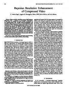
In the first set of experiments, a single frame is synthetically shifted by pixel increments according to f k = C o , mod (k , 4 )f o ,
(11.32)
where fo is the original frame, mod(k,4) is the modulo arithmetic operator that divides k by 4 and returns the remainder, and Co,0 , Co,1 , Co,2 , and Co,3 represent the identity transform, a horizontal pixel shift, a vertical pixel shift, and a diagonal pixel shift, respectively. The original frame is shown in Figure 1, and the goal of the experiment is to establish an upper bound on the performance of the super-resolution algorithm. This is achieved since the experiment ensures that every pixel in the high-resolution image appears in the decimated image sequence. The resulting image sequence is sub-sampled and compressed with an MPEG-4 compliant encoder utilizing the VM5+ rate control mechanism. No filtering is utilized, that is H=I. In the first experiment, a bit-rate of 1 Mbps is employed, which simulates applications with low compression ratios. In the second experiment, a bit-rate of 256 kbps is utilized to simulate high compression tasks. Both experiments maintain a frame rate of 30 frames per second.
Figure 1. Original High Resolution Frame
11. Super-resolution from compressed video
21
An encoded frame from the low and high compression experiments is shown in Figure 2(a) and (b), respectively. Both images correspond to frame 19 of the compressed image sequence and are representative of the quality of the sequence. The original low-resolution frame 19 supplied to the encoder also appears in Figure 2(c). Inspecting the compressed images shows that at both compression ratios there are noticeable coding errors. Degradations in the 1 Mbps experiment are evident in the numbers at the lower right-hand corner of the image. These errors are amplified in the 256 kbps experiment, as ringing artifacts appear in the vicinity of the strong edge features throughout the image. Visual inspection of the decoded data is consistent with the objective peak signal-to-noise ratio (PSNR) metric, which is defined as PSNR =
255 2 1 f − fˆ MN
2
,
(11.33)
where f is the original image and f^ is the high-resolution estimate. Utilizing this error criterion, the PSNR values for the low and high compression
(a)
(b)
(c) Figure 2. Low-Resolution Frame: (a) Compressed at 1 Mbps; (b) Compressed at 256 kbps, and (c) Uncompressed. The PSNR values for (a) and (b) are 35.4dB and 29.3dB, respectively.
22
Chapter 11
images in Figures 2(a) and (b) are 35.4dB and 29.3dB, respectively. With the guarantee that every pixel in the high-resolution image appears in one of the four frames of the compressed image sequence, the superresolution estimate of the original image and high-resolution motion field is computed with (11.29), where TB=1 and TF=2. In the experiments, the shifts in (11.32) are not assumed to be known, but a motion estimation algorithm is implemented instead. However, the motion vectors transmitted in the compressed bit-stream provide the fidelity data. The influence of these vectors is controlled by the parameter , which is chosen as =1. Other ��������� � �� ��� ����� ���� ����� ���� ������������� � ���������� �� ���!�"���� #� �$�!�$���!�$��%� &���� �� � ��'�$��( 1 �����'( in (11.31) and chosen to vary relative to the amount of quantization in 2 ���� � �� ��� $)+*��$�,���� �-�$./���$�0��� �� � �-�$�1� �����!�2 &��� �� �!� ��$� %�( ( =0.1, while for 13 2 ���� 4���!5��6���$�0��� �� � �-���7 &��� �� �!� ��$� �8( ( =0.6. Finally, the relaxation 13 2 ��������� � ��"�-� �� �� �!�� ��1�$�09 )�: ;����� ?� � �� ����� @� algorithm is terminated when _ 3 - ||fln-fln-1||2